Automatic Prediction of High-Resolution Daily Rainfall Fields for ...

1204

JOURNAL OF HYDROMETEOROLOGY

VOLUME 8

Automatic Prediction of High-Resolution Daily Rainfall Fields for Multiple Extents: The Potential of Operational Radar J. M. SCHUURMANS, M. F. P. BIERKENS,

AND

E. J. PEBESMA

Department of Physical Geography, Utrecht University, Utrecht, Netherlands

R. UIJLENHOET Hydrology and Quantitative Water Management Group, Wageningen University, Wageningen, Netherlands (Manuscript received 6 June 2006, in final form 3 January 2007) ABSTRACT This study investigates the added value of operational radar with respect to rain gauges in obtaining high-resolution daily rainfall fields as required in distributed hydrological modeling. To this end data from the Netherlands operational national rain gauge network (330 gauges nationwide) is combined with an experimental network (30 gauges within 225 km2). Based on 74 selected rainfall events (March–October 2004) the spatial variability of daily rainfall is investigated at three spatial extents: small (225 km2), medium (10 000 km2), and large (82 875 km2). From this analysis it is shown that semivariograms show no clear dependence on season. Predictions of point rainfall are performed for all three extents using three different geostatistical methods: (i) ordinary kriging (OK; rain gauge data only), (ii) kriging with external drift (KED), and (iii) ordinary collocated cokriging (OCCK), with the latter two using both rain gauge data and range-corrected daily radar composites—a standard operational radar product from the Royal Netherlands Meteorological Institute (KNMI). The focus here is on automatic prediction. For the small extent, rain gauge data alone perform better than radar, while for larger extents with lower gauge densities, radar performs overall better than rain gauge data alone (OK). Methods using both radar and rain gauge data (KED and OCCK) prove to be more accurate than using either rain gauge data alone (OK) or radar, in particular, for larger extents. The added value of radar is positively related to the correlation between radar and rain gauge data. Using a pooled semivariogram is almost as good as using event-based semivariograms, which is convenient if the prediction is to be automated. An interesting result is that the pooled semivariograms perform better in terms of estimating the prediction error (kriging variance) especially for the small and medium extent, where the number of data points to estimate semivariograms is small and event-based semivariograms are rather unstable.

1. Introduction Rainfall is the main input variable for hydrological models. Hydrologists use spatially distributed hydrological models to gain insight in the spatial variability of soil moisture content, groundwater level as well as the discharge of catchments. As the spatial information on surface elevation, land use, and soil properties increases, hydrologists increase the spatial resolution of these models. However, up to now the spatial resolution of the rainfall input information lags behind. To

Corresponding author address: J. M. Schuurmans, Department of Physical Geography, Faculty of Geosciences, Utrecht University, P.O. Box 80115, 3508 TC Utrecht, Netherlands. E-mail: [email protected] DOI: 10.1175/2007JHM792.1 © 2007 American Meteorological Society

properly model soil moisture content and groundwater level at high resolution, hydrologists require rainfall information to be at high resolution as well. The rainfall information that is readily available for hydrologists in the Netherlands comes from both rain gauges and meteorological radar. All the rainfall data are collected and distributed by the Royal Netherlands Meteorological Institute (KNMI). There are two rain gauge networks, of which the network with the highest density has approximately 1 gauge (100 km2)⫺1 with daily rainfall measured. The operational radar product is a processed composite field of daily rainfall with a resolution of 2.5 km ⫻ 2.5 km from two C-band Doppler radars. If operationally available rainfall data (i.e., rainfall fields from radar and rain gauge data) could be used to

DECEMBER 2007

SCHUURMANS ET AL.

FIG. 1. Locations of weather radars and rain gauges in The Netherlands: two C-band Doppler radars, volunteer network with 330 rain gauges (temporal resolution of 1 day), automatic network with 35 tipping-bucket rain gauges (temporal resolution of 10 min), and experimental network with 30 tipping-bucket rain gauges (equipped with event loggers). The three spatial extents studied are also shown.

1205

correlation in rainfall we restrict ourselves to daily rainfall for two reasons. First, within the Netherlands we have a relatively slow hydrological response to stratiform-dominated rainfall, which means that a temporal resolution of 1 day is already very informative. Second, the operational radar products we use in this study are available at a daily time step. We selected 74 rainfall events and studied for each event the spatial variability of rainfall at three different extents: the small (225 km2), medium (10 000 km2), and large (82 875 km2) extent (i.e., the meso-␥ and meso-␤ scale; Orlanski 1975). We used three geostatistical prediction methods, one using rain gauge data only and the other two combining rain gauge and radar data, and compared the results. The organization of this paper is as follows. In section 2 we describe the data and the event selection procedure. In section 3 the methods are described, starting with variogram modeling, followed by the three geostatistical prediction methods used. The results are given in section 4, starting with the variography (i.e., spatial variability) of rainfall, followed by a case study to show the prediction methods used and finally the cross-validation results are shown. Section 5 deals with the uncertainties of this study. In section 6 we summarize the main conclusions.

2. Data and data processing predict high-resolution rainfall automatically, hydrologists would probably be more willing to use these in their modeling. In this study we therefore focus on using operational radar products that can be readily obtained online from the KNMI. Moreover, we concentrate on prediction procedures that can be automated (i.e., they have to be reliable and robust such that without additional intervention daily predictions are guaranteed). Of course, at the same time the resulting predictions have to be sufficiently accurate to be of any use. Consequently, the main objective of this study is to provide for automatic prediction of rainfall at a high (within a radar pixel) spatial resolution using operational daily rainfall products. Our most important research question is the following: what is the added value of operational radar with respect to rain gauges in terms of rainfall prediction? To predict at a high spatial resolution we need information about the spatial variability of daily rainfall at a small extent. Therefore we have set up an experimental high-density rain gauge network of 30 rain gauges within an area of 225 km2 in the middle of the Netherlands. Although we know that there is a space–time

a. Rain gauge network We used two different kinds of rain gauge networks; one permanent network, which is operated by the KNMI, and one experimental network. Figure 1 shows the location of all the rain gauges of these two networks. The largest network consists of 330 stations and has a density of approximately 1 station (100 km2)⫺1. This network is maintained by volunteers who report the rainfall depth daily at 0800 UTC. These data are available online at the KNMI. The experimental high-density network consists of 30 tipping-bucket rain gauges within an area of 225 km2 in the central part of the Netherlands. The choice for this particular area was based on the fact that several other hydrometeorological experiments are ongoing within this area as well [i.e., the Cabauw Experimental Site for Atmospheric Research (CESAR)], which may be mutually beneficial. Different from the Hydrological Radar Experiment (HYREX), which took place in the United Kingdom between May 1993 and April 1997 (Moore et al. 2000), the purpose of our network was not to give the best estimate of mean rainfall over a radar pixel but in addition to asses the small-extent variability of rainfall (i.e., to estimate the semivariograms of the

1206

JOURNAL OF HYDROMETEOROLOGY

rain fields), in particular, for short lag distances. Therefore, at five locations two rain gauges were placed at very close distance (1–5 m) from each other, a setup that is also recommended by Krajewski et al. (2003). The rest of the gauges were set up in such a way that we had many different intergauge distances. Krajewski et al. (2003) state that knowledge of rainfall structure at spatial extents between a few meters and a few kilometers is still poor. The operationally available rain gauge network in the Netherlands only gives information for distances larger than approximately 10 km, which implies that prediction of high-resolution rainfall fields (smaller than 10 km) is very uncertain. Our highdensity experimental network can be compared with the high-density networks of HYREX, which had 49 tipping-bucket rain gauges within 132 km2 (Moore et al. 2000), and the network of Iowa Institute of Hydraulic Research, which has 15 rain gauges with separation distances ranging from 10 to 1000 m (Krajewski et al. 1998). Our network is therefore unique in the Netherlands and provides valuable information on the spatial structure of rainfall at short distances. For the experimental network we used ARG100 tipping buckets (developed by the Centre for Ecology and Hydrology in the United Kingdom), which are designed to reduce their sensitivity to wind speed and direction, through their aerodynamic design. We placed the rain gauges in open area, free from obstacles. All gauges were equipped with event loggers, that record the momentary tipping event, storing the time and date of each event with a time resolution of 0.5 s. The nominal rainfall accumulation per tipping was 0.2 mm, but a laboratory-derived intensity-dependent correction was made. Approximately every month the loggers were read out and the rain gauges maintained.

b. Radar data The KNMI operates two C-band Doppler radars, one at De Bilt and one at Den Helder, Netherlands (Fig. 1), which both record 288 pseudo CAPPI (800 m) reflectivity fields each day (i.e., every 5 min) after removal of ground clutter (Wessels and Beekhuis 1997). The resolution of these fields is 2.5 km ⫻ 2.5 km. The measured radar reflectivity factor Z (mm6 m⫺3) of each resolution unit is converted to surface rainfall intensity R (mm h⫺1) using the Marshall–Palmer Z–R relationship, which has been found to be most suitable for stratiform-dominated rainfall events (Battan 1973): Z ⫽ 200R1.6.

共1兲

For both radars, the surface rainfall intensities are accumulated from 0800 to 0800 UTC the following day

VOLUME 8

for each pixel. It is known that there is a distancerelated underestimation of surface rainfall by weather radars due to spatial expansion of the radar beam and due to attenuation of the radar signal. Also overestimation due to the bright band (vertical profile of reflectivity) may occur. Therefore, data from the rain gauges of the volunteer network, from the same period, are used to perform a range correction for each radar separately every day (Holleman 2004). This is a rangedependent bias correction and is done as follows (Holleman 2003). Collocated radar (R) and gauge (G) observations form the variable RG, which is only calculated if both the radar and rain gauge measured more than 1-mm rainfall: RG ⬅ 10 log

冉冊

R . G

共2兲

The available RG values are plotted as a function of distance from the radar (r) and a parabola is fitted through this data: RG共r兲 ⫽ a ⫹ br ⫹ cr 2

共3兲

with a, b, and c being the fitting parameters After the range correction, a composite field is constructed by averaging the pixel values of the two radars up to a radius of 200 km away from each radar. Within a radius of 15 km from one radar, the information of the other radar is used. This composite radar field is an operational product of KNMI and is used in this study.

c. Event selection The rain gauges of the experimental network were installed at the beginning of 2004. Between March and October 2004 we selected the 74 events with mean daily rainfall depth of all rain gauges of the experimental network exceeding 1 mm. Rainfall was accumulated from 0800 to 0800 UTC (over a 24-h period) to match the measuring period of the volunteer network and the weather radar. Krajewski et al. (2003) and Steiner et al. (1999) have already mentioned the problems that can occur with rain gauges and we experienced these same problems, resulting in the fact that it was seldom that all 30 rain gauges of the experimental network yielded reliable data simultaneously. We performed a quality check to filter outliers. For each event we made boxand-whisker plots, showing the distribution of the data. Data from rain gauges further than 1.5 times the interquartile range from the nearest quartile were marked as “suspicious” points. Only if it was clear from the fieldwork that these rain gauges showed problems (e.g., clogged up, problems with logger, etc.) they

DECEMBER 2007

SCHUURMANS ET AL.

1207

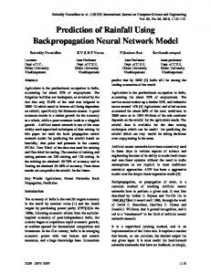
FIG. 2. Gaussian quantile–quantile plots of normalized nonzero rainfall data of the 74 events for three different extents (small, medium, and large extent) and for three transformation scenarios: no transformation (non), log transformation (log), and square root transformation (sqrt).

were removed from the dataset, otherwise the outlier was attributed to spatial variability of the true rainfall field.

d. Data transformation For kriging a (multivariate) Gaussian distribution of the data is preferred. In that case the kriging predictor is the same as the conditional mean and the kriging variance is the same as the variance of the conditional distribution, which makes it possible to calculate ex-

ceedence probabilities from kriging predictions (Goovaerts 1997). To approximate a Gaussian distribution, we tried both a log-transformation and a square root transformation on the data. Only measurements with nonzero rainfall were taken into account and were normalized for each event. Figure 2 shows these transformations for the three different extents. As the square root transformation gave the best results in approximating a Gaussian distribution at all three extents, we chose this transformation for further study.

1208

JOURNAL OF HYDROMETEOROLOGY

3. Methods a. Variogram estimation The semivariogram, from now on simply called the variogram, describes in terms of variances how spatial variability changes as a function of distance and direction (Isaaks and Srivastava 1989). The variogram is needed for kriging. To get insight into the multiextent spatial variability, we distinguished three different spatial extents (Fig. 1); small (225 km2), medium (10 000 km2), and large extent (82 875 km2). The extent is defined in this study as the area over which predictions are made, following Bierkens et al. (2000). In case of no failure, we had data from 30 rain gauges at the small extent, 103 rain gauges at the medium extent (including the 30 from the small-extent network), and 330 rain gauges at the large extent (including the 103 from the medium-extent network).

1) INDIVIDUAL

VARIOGRAMS

For each of the 74 events we calculated the experimental variogram of the square root transformed rain gauge data. The experimental variogram is calculated as half the average squared difference between the paired data values, so in case of square root–transformed rain gauge measurements G(xi),

␥ˆ 共h兲 ⫽

1 2N共h兲

N共h兲

兺 关G共x 兲 ⫺ G共x ⫹ h兲兴 , 2

i

i

共4兲

i⫽1

in which N(h) is the number of point pairs and h the separation distance. The maximum separation distance considered is taken as 1⁄3 of the extent (i.e., 8, 50, and 150 km for the small, medium, and large extent, respectively). The reason for that is that point pairs with a larger separation distance are too highly correlated (Journel and Huijbregts 1978). Up to the maximum separation distance we chose 15 distance intervals into which data point pairs were grouped for semivariance estimates. To assure that the kriging equations have a unique and stable solution (i.e., to force the variogram to be positive definite) we have to fit a suitable variogram model (Isaaks and Srivastava 1989) to the experimental variogram. Among several models, we chose the widely used spherical variogram model, defined as

␥共h兲 ⫽

冦

C0关1 ⫺ ␦k共h兲兴 ⫹ C C0 ⫹ C

冉

h3 3h ⫺ 3 2a 2a

冊

0ⱕhⱕa h ⬎ a, 共5兲

VOLUME 8

in which the Kronecker delta function ␦k(h) is 1 for h ⫽ 0 and 0 for h ⬎ 0. The parameter C0 is the nugget variance, C is the partial sill, and a is the range of the spherical variogram model. The parameters of the spherical variogram models were fitted automatically with nonlinear regression, using weights N(h)/h2 with N(h) as the number of point pairs and h as the distance. This criterion is partly suggested by theory, and partially by practice (Pebesma 2004). When it was not possible to fit a unique variogram model, the range was forced to be beyond the extent. All geostatistical operations were carried out using the package gstat (Pebesma 2004) within R (R Development Core Team 2004).

2) POOLED

VARIOGRAMS

Without the experimental rain gauge network, hydrologists should extract information about the smallscale rainfall variability from the KNMI network. As mentioned in section 2 these networks do not give insight into the spatial variability of rainfall at distances smaller than approximately 10 km. To be able to make high-resolution predictions of rainfall in spite of that, we computed a single pooled variogram for each extent based on all the 74 selected events, including the information of the experimental rain gauge network. For each event we performed kriging predictions using both the individual variogram model for that event as well as the pooled variogram model and compared the results. This way we can draw conclusions about whether it is permitted to use one standard variogram model, which would be helpful for automated prediction.

b. Prediction methods This section introduces briefly three geostatistical prediction methods that were used for this study. The first method uses only rain gauge information while the second and third method use both rain gauges and radar information but in a different manner. For more detailed information readers are referred to Isaaks and Srivastava (1989), Goovaerts (1997), and Cressie (1993).

1) ORDINARY

KRIGING

Geostatistical prediction is based on the concept of a random function, whereby the unknown values are regarded as a set of spatially dependent random variables. Kriging is a generalized least squares regression technique that allows one to account for the spatial dependence between observations, as revealed by the variogram, in spatial prediction. Kriging is associated

DECEMBER 2007

1209

SCHUURMANS ET AL.

with the acronym BLUP, meaning “best linear unbiased predictor” (Cressie 1993). It is “linear” as the estimated values are weighted linear combinations of the available data. It is “unbiased” because the expectation of the error is 0 and it is “best” as it minimizes the variance of the prediction errors. The ordinary kriging ˆ ) at the unprediction of square root rainfall (R OK sampled location x0 is a linear combination of the n neighboring square root transformed rain gauge observations G(xi):

The trend coefficients (a0 and a1) are implicitly estimated through the kriging system within each search neighborhood using generalized least squares. In our case the search neighborhood was not fixed but depended on the available data points. At maximum 40 neighboring points are taken into account. The kriging with external drift prediction of square root rainfall ˆ (R KED) at the unsampled location x0 is n

ˆ R KED共x0 兲 ⫽

ˆ 共x 兲 ⫽ R OK 0

兺 ␭ G共x 兲. i

i

共6兲

i⫽1

ˆ The weights ␭i must be such that the predictor R OK is 1) unbiased (i.e., giving no systematic under or overestimation) and 2) optimal (i.e., with a minimal mean squared error). These weights are obtained by solving

冦

n

兺 ␭ ␥共x ⫺ x 兲 ⫺ ␮ ⫽ ␥共x ⫺ x 兲 j

i

j

i

0

i ⫽ 1, . . . , n

j⫽1

n

兺 ␭ ⫽ 1,

共7兲

j

j⫽1

with ␮ being the Lagrange parameter accounting for the unbiasedness constraint on the weights. The only information needed to solve the kriging system [Eq. (7)] are the semivariogram values, which can be calculated from the fitted variogram model [Eq. (5)].

2) KRIGING

WITH EXTERNAL DRIFT

i

共9兲

i

The weights of kriging with external drift are obtained by solving the system:

冦

n

兺␭␥

j res共xi

⫺ xj兲 ⫹ ␮0 ⫹ ␮1R共xi兲 ⫽ ␥res共xi ⫺ x0兲

j⫽1

共8兲

i ⫽ 1, . . . , n n

兺␭ ⫽1 j

j⫽1

n

兺 ␭ R共x 兲 ⫽ R共x 兲, j

j

0

j⫽1

共10兲

with ␮0 and ␮1 being the Lagrange parameters accounting for the unbiasedness constraints on the weights. Kriging with external drift is performed using ␥res as the variogram of the residuals from the trend.

3) ORDINARY

Beyond using information from the rain gauges G(xi) only, kriging can use secondary information to improve the kriging prediction (Goovaerts 1997). In case of rainfall, an informative secondary data source is the square root rainfall estimated by the weather radar (R). We used two kriging algorithms that incorporate exhaustively sampled secondary data: 1) kriging with external drift (KED) and 2) ordinary collocated cokriging (OCCK). KED is comparable to universal kriging (kriging with a trend): we assume that we know the shape of the trend and kriging is then performed on the residuals while the trend parameters are implicitly estimated. In universal kriging the trend is often a function of internal variables (coordinates) while in KED the trend surface is based on a trend through the secondary data (external variables). Mathematically they are identical. Although the trend can be a linear regression through several external variables, we only considered radar R(x) as secondary data: m共x兲 ⫽ a0 ⫹ a1R共x兲.

兺 ␭ G共x 兲. i⫽1

n

COLLOCATED COKRIGING

Another algorithm for taking into account secondary information is OCCK. Different from KED in which the secondary data provides information on the trend only, in OCCK the secondary data, which is now considered as a random variable as well, influences the kriging prediction directly. In addition, OCCK accounts for the global linear correlation between primary and secondary variables, whereas with KED the secondary information tends to strongly influence the prediction, especially when the estimated slope or intercept of the local trend model is large. A more or less similar and more well-known kriging method using secondary information is ordinary cokriging (OCK). Several studies have used OCK to merge rain gauge and radar rainfall: Creutin et al. (1988), Fiorucci et al. (2001), Krajewski (1987), and Seo et al. (1990a,b). Goovaerts (2000) incorporated elevation as secondary information and tested several kriging methods that account for secondary data. OCCK is preferred to OCK for the following four reasons (Goovaerts 1997): 1) OCCK avoids instability caused by

1210

JOURNAL OF HYDROMETEOROLOGY

VOLUME 8

highly redundant secondary data, 2)OCCK is faster than OCK as it calls for a smaller cokriging system, 3) OCCK does not call for a secondary covariance function at distances larger than 0, and 4) OCCK does not require modeling of the cross-covariance function by using the Markov-type approximation (i.e., dependence of the secondary variable on the primary is limited to the collocated primary datum). The ordinary collocated cokriging prediction of ˆ square root rainfall (R OCCK) at the unsampled location x0 is a linear combination of the n neighboring square root–transformed rain gauge observations G and one collocated square root–transformed radar observation R: n

ˆ R OCCK共x0 兲 ⫽

兺 ␭ G共x 兲 ⫹ ␰R共x 兲, i

i

0

共11兲

i⫽1

with the constraint that the weights (兺ni⫽1 ␭i ⫹ ␰) sum to 1. In case the expected value of the primary and secondary data are not equal, Eq. (11) must be adjusted, so the secondary data is bias corrected. In our case we assumed the expected values of the rain gauges and radar to be the same because the operational radar are already bias corrected (section 2b). The ordinary collocated cokriging weights are obtained by solving the system:

冦

n

兺␭␥

j GG共xi

⫺ xj兲 ⫹ ␰␥GR共xi ⫺ x0兲 ⫹ ␮ ⫽ ␥GG共xi ⫺ x0兲

j⫽1

i ⫽ 1, . . . , n n

兺␭␥

j GR共x0

⫺ xj兲 ⫹ ␰␥RR共0兲 ⫹ ␮ ⫽ ␥GR共0兲

FIG. 3. Box-and-whisker plots of the standard deviation of nonzero rainfall at the three spatial extents for the 74 events. The black dot denotes the median, solid boxes range from the lower to the upper quartile, and dashed whiskers show the data range. Data that are further than 1.5 times the interquartile range from the nearest quartile are shown as open bullets.

radar data. The cross variogram (␥GR) was calculated by multiplying the direct variogram of the rain gauges (␥GG) with the correlation between the collocated square root–transformed rain gauge and radar data, assuming the Markov-type approximation (Goovaerts 1997).

j⫽1

c. Back transformation and zero rainfall

n

兺

␭j ⫹ ␰ ⫽ 1,

j⫽1

共12兲

with ␮ being the Lagrange parameter accounting for the unbiasedness constraints on the weights, ␥GG is the direct variogram of the rain gauge data, ␥GR is the cross variogram of rain gauge and radar data, and ␥RR is the direct variogram of the radar data. The three variograms are modeled as a linear combination of the same basic model, the fitted spherical variogram model of the normalized square root– transformed rain gauge data [Eq. (5)]. The direct variogram of the rain gauges (␥GG) was calculated by multiplying the standardized variogram with the variance of the square root–transformed rain gauge measurements. The direct variogram of the radar data (␥RR) was calculated by multiplying the standardized variogram by the variance of the square root–transformed

Rainfall can be considered as a binary process, it either rains or it does not. As shown in Fig. 2 the measurements of nonzero daily rainfall closely follow a Gaussian distribution after a square root transformation. Kriging performs best when data are (multivariate) Gaussian distributed and we therefore applied kriging to the nonzero, square root–transformed (nonstandardized) rainfall measurements. This means that the ordinary kriging prediction and collocated cokriging prediction are best in predicting the square root rainfall given that it rains. To obtain back-transformed rainfall values we cannot simply take the square of the kriging prediction based on the square root–transformed rainfall data. The reason for this is that if a Gaussian distribution is squared, it becomes positively skewed, resulting in a mean larger than the median. Simply squaring the kriging prediction of square root– transformed rainfall data would underestimate the con-

DECEMBER 2007

SCHUURMANS ET AL.

1211

FIG. 4. Small-extent normalized variograms of square root–transformed daily rainfall with fitted spherical model for each of the 74 events in 2004 (header in “month month day day,” e.g., 0306 means 6 March). For 17 and 21 Aug 2004, the automatically fitted variogram model is outside the plotted semivariance range.

ditional mean of rainfall, especially in case of large kriging variances. To back transform prediction values we therefore calculated the percentiles of the conditional distribution of square root–transformed rainfall, assuming this distribution to be Gaussian with mean equal to the kriging prediction and variance equal to the kriging variance. After that we back-transformed (squared) these percentiles, whose rank and percentile value do not change with transformation. From this new distri-

bution function we calculated the mean and the variance. By not considering the number of zeroes in the dataset valuable information would be lost. Therefore we forced the predicted rainfall values to contain the same percentage of zero’s as in the dataset. The predicted rainfall amounts were arranged in increasing order and a threshold was calculated that corresponded with the percentage of zeroes in the rainfall dataset. All

1212

JOURNAL OF HYDROMETEOROLOGY

VOLUME 8

FIG. 5. Same as in Fig. 4, but for the medium extent.

the prediction locations with rainfall smaller than this threshold were set to zero.

4. Results a. Variograms To compare the spatial structure of each event in one plot we calculated the variograms of the normalized (i.e., variance equals 1) square root–transformed rainfall data. The variance in rainfall however, differs between both the events and extents. Figure 3 shows in a

box-and-whisker plot for each extent the standard deviation of nonzero (nonnormalized and nontransformed) rainfall for all the 74 events. This figure shows a positive trend in the variability of nonzero rainfall from a small to larger extent. Figure 4, 5, and 6 show for each event the normalized experimental variograms of the square root–transformed daily rainfall, as well as the automatically fitted spherical variogram model of respectively the small, medium, and large extent. In Fig. 4 the fitted variogram model for 17 and 21 August (0817 and 0821, respec-

DECEMBER 2007

SCHUURMANS ET AL.

1213

FIG. 6. Same as in Fig. 4, but for the large extent.

tively) is outside the plotted semivariance range. During those days there was a high semivariance between point pairs with the smallest separation distance, causing our automated procedure to fit a variogram model with a large nugget. Due to the larger data availability at larger extents, the experimental variograms become less ambiguous and the variogram models fit better. Figure 7 shows the fitted ranges of the spherical variogram models for each event for the small, medium, and large extent. This figure shows a large variability in fitted ranges across events, but a seasonal effect is not

clear. Figure 7 also shows the fitted range of the spherical variogram model for the small and medium extent to be often 25 and 150 km, respectively, which are the values that were enforced when the nonlinear variogram fitting procedure was not successful. Figure 8 shows the experimental pooled variograms as well as the fitted spherical variogram models of the small, medium, and large extent. For the medium and large extent we fitted a nested spherical variogram model (i.e., a sum of two spherical variogram models; Deutsch and Journel 1998). The parameters

1214

JOURNAL OF HYDROMETEOROLOGY

VOLUME 8

FIG. 7. Automatically fitted ranges (km) of spherical variogram models for small, medium, and large extent as a function of the event date.

of the fitted spherical variogram models are given in Table 1. The pooled variogram model was calculated using normalized square root–transformed daily rainfall data. For the kriging prediction, the nugget and sill of the variogram model should be multiplied by the variance of the square root–transformed daily rainfall data.

b. Rainfall prediction 1) CASE

STUDY

Figure 9 shows the accumulated daily composite range-corrected radar field for the period March– October 2004 at the small extent. During this period, 22 radar images were either missing or incomplete. From this figure is can be seen that even for an accumulation period of 7 months, there still is a difference of 10%

rainfall within the small extent. This corroborates our argument that for the Netherlands a temporal resolution of 1 day is important even at a small extent. To demonstrate the kriging methods described in the preceding paragraphs we selected two of the 74 rainfall events: 4 April and 1 May 2004. Figure 10 shows the composite range-corrected radar fields for the selected dates. These two events were chosen because they represent two different rainfall types with different correlation between rain gauge data and radar. The event of 4 April 2004 is an example of a stratiform event because it rains over a large area and extremely high rainfall areas cannot be detected. The event of 1 May 2004 is an example of a convective event because the rainfall area is smaller and high rainfall values are present. Figure 11 shows the prediction of rainfall depth at the small extent for 4 April 2004 according to the range

DECEMBER 2007

1215

SCHUURMANS ET AL.

FIG. 8. Pooled variogram models of the small, medium, and large extent, calculated from the standardized nonzero square root–transformed daily rainfall data. For the medium and large extent a nested spherical variogram model is fitted.

corrected radar, the ordinary kriging prediction, kriging with external drift prediction, and the ordinary collocated cokriging prediction, respectively. The kriging predictions are made at a high-resolution point grid with distances of 100 m. For the medium and large extent we only used the 40 nearest data points instead of the complete dataset for kriging. For this event the correlation between the rainfall measured by the rain gauges and the collocated radar at the small extent was 0.16. Because of this low correlation, the trend surface of the radar has a very small effect on the KED prediction. For the ordinary collocated cokriging prediction, however, the radar field can be clearly seen. This is due to the fact that for each prediction location within a radar pixel this same collocated radar value is taken into account [Eq. (11)]. Within the radar pixel

itself, the rainfall depths are interpolated. To overcome the problem of sudden transitions in rainfall depth from one radar pixel to the other, the radar field can be presmoothed before executing the KED or OCCK. We TABLE 1. Parameters of fitted pooled spherical variogram models. Here C1 and a1 are the partial sill and range, respectively, of the first variogram model. In case of a nested variogram model C2 and a2 are the partial sill and range, respectively, of the second variogram model [see Eq. (5)]. Parameter

Small extent

Medium extent

Large extent

C0 C1 C2 a1 (km) a2 (km)

0.172 1.270 — 10 —

0.035 0.473 8.994 20 1040

0.053 0.281 0.795 23 156

1216

JOURNAL OF HYDROMETEOROLOGY

FIG. 9. Total rainfall during March–October 2004 at a small extent according to daily range-corrected radar.

retrieved good results by smoothing the radar with inverse distance interpolation using the four closest grid cell center points of the radar field. Figure 12 shows the rainfall fields using the same kriging methods for the 1 May 2004 event. For this event the correlation between the rainfall measured by the rain gauges and the collocated radar at the small extent was 0.84. In Figs. 11 and 12 we show the predicted rainfall depths using OK, KED, and OCCK for the small extent. We assumed that for all events it rained throughout the whole small extent so we did not have to cope with the problem of zero rainfall.

VOLUME 8

To illustrate how our method deals with zero rainfall, we show the rainfall depths of the different methods for 1 May 2004 at the large extent in Fig. 13. During this event 114 rain gauge stations out of the 211 reported zero rainfall. We forced the same percentage (54%) of the prediction locations to have zero rainfall. From this figure it can be seen that, using ordinary kriging (OK), rainfall is predicted in the northern part of the Netherlands where the radar did not detect rainfall, whereas in the southern part ordinary kriging does not predict rainfall where the radar does detect rainfall. KED and OCCK combine the two sources of information, but in a slightly different manner. In this case, the predictions of both methods follow the spatial rainfall structure as shown by the radar. The rainfall measured by the rain gauges in the northern part of the Netherlands was so low that it was set to zero.

2) CROSS

VALIDATION

To compare the accuracy of the three different kriging forms (OK, OCCK, and KED) as well as the use of either the individual variogram models or pooled variogram models, we used cross validation. The idea of cross validation is to remove one data point at a time from the dataset and repredict this value from the remaining data. For each extent and event we performed cross validation, using the three different kriging forms. For ordinary kriging as well as ordinary collocated cokriging we used both the individual variogram model of that event (e.g., Fig. 4) as well as the pooled variogram model (Fig. 8) of that extent. Finally, for each event we calculated the root-mean-squared error (rmse) resulting from the cross-validation calculations.

FIG. 10. Composite range-corrected radar fields of (left) 4 Apr and (right) 1 May 2004.

DECEMBER 2007

SCHUURMANS ET AL.

1217

FIG. 11. Prediction of rainfall depth at small extent for 4 Apr 2004 according to the range-corrected radar (radar), OK pred, KED pred, and OCCK pred. Green triangles show the rain gauge locations. Radar–rain gauge correlation is 0.16.

In our case study of 74 events, we had 7 incomplete radar fields, due to technical malfunction or maintenance of one of the radars. These events were not taken into account in the cross validation. The distributions of the rmse resulting from the cross validation using the different kriging methods are plotted in box-andwhisker plots (Fig. 14). We also calculated the rmse of the difference between the rainfall measured by the rain gauges and the collocated radar pixel and these results (radar) are shown as well in Fig. 14. Figure 14 shows that taking into account radar as secondary variable, using either KED or OCCK, leads to better results than only taking into account data from rain gauges for the medium and large extent. Also, for the medium and large extent, radar performs better than rain gauge data alone (OK). For the small extent, however, the rain gauge data alone perform better and the added value of taking into account radar is not so clear.

This is not surprising as we have a dense network of rain gauges at the small extent. The use of a pooled variogram model for all events instead of individual variogram models for each separate event makes little difference. For the small extent the pooled variogram model performs less than the individual variogram models whereas for the medium and large extent it is the other way around. Figure 15 shows the ratio between the rmse as calculated with OK and KED (ratio.rmse.ok.ked, shown as ⫹) as well as the ratio between the rmse as calculated with OK and OCCK (ratio.rmse.ok.cck, shown as o) as a function of the correlation between rain gauges and radar for the small, medium, and large extent. If the ratio is higher than 1, it means that KED or OCCK performs better than OK. Again we see that the larger the extent, the higher the added value of the radar. Figure 15 also shows the positive effect of the correla-

1218

JOURNAL OF HYDROMETEOROLOGY

VOLUME 8

FIG. 12. Same as in Fig. 11, but for 1 May 2004. Radar–rain gauge correlation is 0.84.

tion between radar and rain gauge and the ratio of rmse, especially at the medium and large extent. We also looked at the z score of the cross-validation exercise, which is the residual divided by kriging standard error. The z score should have zero mean and unit variance. If the mean z score deviates from zero, we have a biased prediction, and if the variance is higher than 1, we underestimate the kriging variance. For each event we calculated the mean z score using the three different kriging methods. The results are shown in a box-and-whisker plot (Fig. 16). It can be seen that for almost all events and kriging methods, the mean z score is close to zero, except for OCCK. This is probably due to our assumption that the expected value of the rain gauge data and radar data are the same. Figure 17 shows in a box-and-whisker plot the variance of the z score that we calculated for each event using the three kriging methods. It is most striking that the pooled variogram used for both OK and OCCK leads to lower

z-score variances and thus better estimation of the prediction error variance.

5. Discussion In this section we deal with some remaining uncertainties and possible improvements of the methods presented in this paper. This paper deals with daily rainfall. For hydrological applications it would be interesting to also be able to generate high spatial resolution rainfall fields with a higher time resolution (e.g., 3 h). In that case the main problem we would have to cope with is the reduction of the amount of rain gauge measurements, as the largest operational rain gauge network in The Netherlands consists of volunteers who only report the daily rainfall depth. Consequently the present range correction of the weather radar cannot be performed on a higher time resolution, as this method uses the volunteer net-

DECEMBER 2007

SCHUURMANS ET AL.

1219

FIG. 13. Same as in Fig. 11, but for the Netherlands on 1 May 2004.

work as well. With a low-density rain gauge network our method to correct for zero rainfall is also not suitable because an individual rain gauge reporting zero rainfall would have too much influence. Besides the fact of the decrease in rain gauge stations we would also have to deal with the following problems: (i) the cor-

relation between rainfall measured by the rain gauges and radar is known to decrease at small time scales, especially when (e.g., in convective rainfall) there is a large space–time variability of rainfall; (ii) reestimation of the variogram models as it is known that for rainfall averaged over larger spatial scales and integrated over

1220

JOURNAL OF HYDROMETEOROLOGY

VOLUME 8

FIG. 14. Box-and-whisker plots of the rmse of the residuals from the comparison between operational radar and rain gauges (radar) as well as the rmse of the residuals from the cross validation using three kriging methods: OK, OCCK, and KED. For both OK and OCCK we used the individual variograms (indiv) as well as the pooled variograms (pooled).

longer periods the correlation distance is typically larger; and (iii) reconsideration of the square root transformation of rainfall data to make its distribution closer to Gaussian. Possibly for shorter periods a logarithmic transformation would be more suitable. For shorter time steps, the spatial continuity of radar measurements becomes a major advantage compared to rain gauge networks. This however does not preclude the thorough radar data processing [e.g., correction for vertical profile of reflectivity (VPR) and attenuation] required to improve as far as possible the radar data quality. Besides all the advantages of using radar data, it is important to recognize the inherent limitations of radar data quality, especially as a function of range. The

average range limit to keep in mind for hydrological use of weather radar is on the order of 80 km. Results from HYREX show that distributed hydrological models are sensitive to rain gauge location and hence to the spatial variability of rainfall over the catchment, especially during convective rainfall (Bell and Moore 2000). In the Netherlands, convective rainfall mainly occurs during summer as a result of local ascent of warm air and is characterized by heavy rainfall with a small spatial extent and a short duration. During wintertime, stratiform rainfall events dominate caused by frontal systems. They have a larger spatial extent than convective rainfall, as well as a longer lifetime. For this reason, our initial purpose was to divide the events into

DECEMBER 2007

SCHUURMANS ET AL.

1221

FIG. 15. Ratio of the rmse as calculated with ordinary kriging and kriging with external drift (rmse.OK/ rmse.KED, shown as ⫹) as well as the ratio of the rmse as calculated with ordinary kriging and ordinary collocated cokriging (rmse.OK/rmse.CCK, shown as 䊊) as function of the correlation between rain gauges and radar for the small, medium, and large extent. Dashed line represents the value 1.

two rainfall types (convective and stratiform) and to pool the variograms for each rainfall type, instead of using only one pooled variogram model for each extent. To identify convective areas we applied the algorithm proposed by Steiner et al. (1995) to 5-min CAPPI radar fields using the same criteria as stated in their paper. In case the majority of the grid cells within the extent were identified at least 10 times as convective during that day, we labeled the event as convective, otherwise it was classified as stratiform. However, when we pooled the variograms per rainfall type we did not find sufficient differences between the form of the pooled variograms to justify the separated modeling. Further research is required to investigate whether a separate

modeling of stratiform and convective events is required and if so, how to better distinguish between stratiform and convective events. Although we are aware of the directional variability in rainfall fields we did not consider anisotropy in our variogram model fits, mostly because we had too little data points within our small extent. The 30 data points we had at maximum for each event at the small extent are the absolute minimum to fit an omnidirectional variogram, but provide insufficient information to estimate directional variograms. This was also the case for the medium extent. An additional reason not to use directional variograms is that estimating them and fitting suitable models, is difficult to reconcile in an au-

1222

JOURNAL OF HYDROMETEOROLOGY

VOLUME 8

FIG. 16. Box-and-whisker plots of the mean z score from the cross validation using three kriging methods: OK, OCCK, and KED. Dashed line represents the value zero. For both OK and OCCK we used the individual variograms (indiv) as well as the pooled variograms (pooled).

tomatic fashion. Moreover, using a kriging method that takes into account the secondary data of the radar, will take into account the existing anisotropy present in the radar image. Kriging predictions were made using either the individual variogram models or the pooled variogram model. We did not take into account the quality of the variogram model fit. This can be done by using for instance Markov Chain Monte Carlo techniques (Diggle et al. 1998). Probably, the effect on kriging prediction would not be large if we have enough data but it becomes relevant for sparse rain gauge networks. We applied OCCK assuming that the Markov-type approximation (Goovaerts 1997) holds, in order to

make the automatic prediction procedure faster. It should be possible to automatically calculate and fit the cross-covariance function and implement this in the OCCK procedure. This is, however, beyond the scope of this paper. Kriging with external drift as applied in this paper, assumes the secondary data to be free from errors. A possible improvement could be to use external drift kriging with uncertain covariates (Van de Kassteele and Stein 2006).

6. Conclusions We show that kriging with external drift and ordinary collocated cokriging successfully take into account ra-

DECEMBER 2007

SCHUURMANS ET AL.

1223

FIG. 17. Same as in Fig. 16, but for the variance of the z score. Dashed line represents the value 1.

dar as a secondary information source and are more accurate than ordinary kriging (rain gauge information only), especially for larger extents with lower densities of rain gauges. The added value of radar is positively related to the correlation between the rainfall measured by the rain gauges and the collocated radar pixel. The use of a pooled variogram model instead of an individual variogram model for each event does not lead to a loss of accuracy in rainfall prediction, so these pooled variogram models can be used when there is lack of data or when an automatic prediction procedure is implemented without variogram estimation. We also show that the pooled variogram is preferred over event-based variograms in terms of correct assessment of prediction uncertainty (z score variance of 1)

for the small- and medium-extent cases, where the number of data is small and event-based variograms are rather uncertain. Another conclusion is that KED and OK are more robust with respect to mean z scores (on average zero) than OCCK. This may be due to a bias in the radar data. Acknowledgments. The authors would like to thank the Royal Netherlands Meteorological Institute (KNMI), in particular Iwan Holleman and Ton Donker, for their help and for providing us with their data. J. M. Schuurmans was financially supported by TNO and R. Uijlenhoet was financially supported by the Netherlands Organization of Scientific Research (NWO) through Grant 016.021.003. We also acknowledge the reviewers for their valuable comments.

1224

JOURNAL OF HYDROMETEOROLOGY REFERENCES

Battan, L. J., 1973: Radar Observations of the Atmosphere. University of Chicago Press, 319 pp. Bell, V. A., and R. J. Moore, 2000: The sensitivity of catchment runoff models to rainfall data at different spatial scales. Hydrol. Earth Syst. Sci., 4, 653–667. Bierkens, M., P. Finke, and P. de Willigen, 2000: Upscaling and Downscaling Methods for Environmental Research. Kluwer Academic Publishers, 190 pp. Cressie, N. A. C., 1993: Statistics for Spatial Data. rev. ed. John Wiley & Sons, 900 pp. Creutin, J. D., G. Delrieu, and T. Lebel, 1988: Rain measurements by rain gauge–radar combination: A geostatistical approach. J. Atmos. Oceanic Technol., 5, 102–115. Deutsch, C. V., and A. G. Journel, 1998: GSLIB: Geostatistical Software Library and User’s Guide. 2d ed. Oxford University Press, 369 pp. Diggle, P. J., J. A. Tawn, and R. A. Moyeed, 1998: Model-based geostatistics. J. Roy. Stat. Soc. Appl. Stat., 47C, 299–326. Fiorucci, P., P. La Barbera, L. G. Lanza, and R. Minciardi, 2001: A geostatistical approach to multisensor rain field reconstruction and downscaling. Hydrol. Earth Syst. Sci., 5, 201– 213. Goovaerts, P., 1997: Geostatistics for Natural Resources Evaluation. Oxford University Press, 500 pp. ——, 2000: Geostatistical approaches for incorporating elevation into the spatial interpolation of rainfall. J. Hydrol., 228, 113– 129. Holleman, I., 2003: Neerslaganalyse uit radar-en stationswaarnemingen (Rainfall analysis from radar and raingauge measurements). Royal Netherlands Meteorological Institute (KNMI), Tech. Rep. TR-272, 24 pp. ——, 2004: VPR adjustment using a dual CAPPI technique. Proc. Third European Conf. on Radar Meteorology (ERAD), Vol. 2, Visby, Island of Gotland, Sweden, Copernicus GmbH, 25– 30. Isaaks, E. H., and R. M. Srivastava, 1989: Applied Geostatistics. Oxford University Press, 561 pp. Journel, A. G., and C. J. Huijbregts, 1978: Mining Geostatistics. Academic Press, 600 pp.

VOLUME 8

Krajewski, W. F., 1987: Cokriging radar-rainfall and rain gage data. J. Geophys. Res., 92 (D8), 9571–9580. ——, A. Kruger, and V. Nespor, 1998: Experimental and numerical studies of small-scale rainfall measurements and variability. Water Sci. Technol., 37, 131–138. ——, G. J. Ciach, and E. Habib, 2003: An analysis of small-scale rainfall variability in different climatic regimes. Hydrol. Sci. J., 48 (2), 151–162. Moore, R. J., D. A. Jones, D. R. Cox, and V. S. Iham, 2000: Design of the HYREX raingauge network. Hydrol. Earth Syst. Sci., 4, 523–530. Orlanski, I., 1975: A rational subdivision of scales for atmospheric process. Bull. Amer. Meteor. Soc., 56, 527–530. Pebesma, E. J., 2004: Multivariable geostatistics in S: The gstat package. Comput. Geosci., 30, 683–691. R Development Core Team, 2004: R: A language and environment for statistical computing. R Foundation for Statistical Computing, Vienna, Austria. [Available online at http:// www.R-Project.org.] Seo, D. J., W. F. Krajewski, A. Azimizonooz, and D. S. Bowles, 1990a: Stochastic interpolation of rainfall data from rain gauges and radar using cokriging. 2. Results. Water Resour. Res., 26, 915–924. ——, ——, and D. S. Bowles, 1990b: Stochastic interpolation of rainfall data from rain gauges and radar using cokriging. 1. Design of experiments. Water Resour. Res., 26, 469–477. Steiner, M., R. A. Houze, and S. E. Yuter, 1995: Climatological characterization of three-dimensional storm structure from operational radar and rain gauge data. J. Appl. Meteor., 34, 1978–2007. ——, J. Smith, S. Burges, C. Alonso, and R. Darden, 1999: Effect of bias adjustment and rain gauge data quality control on radar rainfall estimation. Water Resour. Res., 35, 2487–2503. Van de Kassteele, J., and A. Stein, 2006: A model for external drift kriging with uncertain covariates applied to air quality measurements and dispersion model output. Environmetrics, 17, 309–322. Wessels, H. R. A., and J. H. Beekhuis, 1997: Stepwise procedure for suppression of anomalous ground clutter. Proc. COST-75 Seminar on Advanced Radar Systems, EUR 16013 EN, Brussels, Belgium, European Commission, 270–277.