Automatically Induced Syntactic Transfer Rules for Machine

Automatically Induced Syntactic Transfer Rules for Machine Translation under a Very Limited Data Scenario

A Dissertation submitted to the graduate school in partial fulfillment of the requirements for the degree Doctor or Philosophy in Language and Information Technologies by KATHARINA PROBST Committee: Alon Lavie (chair) Jaime Carbonell Lori Levin Bonnie Dorr, University of Maryland, College Park Language Technologies Institute School of Computer Science Carnegie Mellon University Pittsburgh, Pennsylvania, U.S.A. March 19, 2005

2

Abstract

The rule-based approach to machine translation (MT) captures structural mappings between the source language and the target language, with the goal of producing grammatical translations. The major drawback of the approach is the development bottleneck, requiring many human-years of rule development. On the other hand, data-driven approaches such as example-based and statistical MT achieve fast and robust system development by deriving mostly non-structural translation information from bilingual corpora. This thesis aims at striking a balance between both approaches by inferring transfer rules automatically from bilingual text, aiming specifically at scenarios when bilingual data is in sparse supply. The rules are learned using a variety of information given, such as parses, part of speech tags, etc. that are available for one of the languages. They are learned in three stages, first producing an initial hypothesis, then capturing the syntactic structure, and finally adding appropriate unification constraints. The learned rules are used in a run-time translation system, a statistical transfer system which is a combination of a transfer engine and a statistical decoder. We demonstrate the algorithms in a Hebrew→English translation task. The main contribution of this thesis is a new framework and a thorough investigation of the problem of inferring structural information with feature constraints from bilingual text. The framework can be used for any language pair, and the inferred information can, after some system-specific adaptation, be used in conjunction with statistical as well as example-based MT systems. Since my thesis work targets language pairs with very little available data, the inferred rules can provide an additional source of information for these systems. Further, the thesis pushes the community into the direction of inferring information from very small training corpora, and provides methods to do so.

Contents 1 Introduction and Motivation

7

2 Thesis Statement

9

3 Related Work and Setting 3.1 Related Work Within and Outside the Avenue Project . . . . . 3.1.1 Transfer Rule Formalism . . . . . . . . . . . . . . . . . . . 3.1.2 Transfer Engine . . . . . . . . . . . . . . . . . . . . . . . . 3.1.3 Run-Time System and Complete Avenue Project Overview 3.2 Training Data . . . . . . . . . . . . . . . . . . . . . . . . . . . . . 3.2.1 Functional Elicitation Corpus . . . . . . . . . . . . . . . . 3.2.2 Structural Training Corpus . . . . . . . . . . . . . . . . . 3.2.3 Training Data Format . . . . . . . . . . . . . . . . . . . . 3.2.4 A Note on Uncontrolled Corpora . . . . . . . . . . . . . . 3.2.5 Evaluation Methodology . . . . . . . . . . . . . . . . . . .

11 11 12 16 17 19 19 20 22 23 23

4 Seed Generation 4.1 Introduction . . . . . . . . . . . . . . . 4.2 Description of Learning Algorithm . . 4.3 Results . . . . . . . . . . . . . . . . . . 4.3.1 Discussion of Learned Rules . . 4.3.2 Automatic Evaluation Results .

27 27 27 29 29 31

. . . . .

. . . . .

. . . . .

. . . . .

. . . . .

. . . . .

. . . . .

. . . . .

. . . . .

. . . . .

. . . . .

. . . . .

. . . . .

. . . . .

. . . . .

5 Structural Learning 5.1 Introduction . . . . . . . . . . . . . . . . . . . . . . . . . . . . . . 5.2 Taxonomy of Structural Mappings . . . . . . . . . . . . . . . . . 5.2.1 System Constraints . . . . . . . . . . . . . . . . . . . . . . 5.2.2 General Space of Possible Mappings . . . . . . . . . . . . 5.2.3 Space Defined by Rule Formalism . . . . . . . . . . . . . 5.2.4 Space Defined by Learning Setting . . . . . . . . . . . . . 5.3 The Basic Compositionality algorithm . . . . . . . . . . . . . . . 5.4 Approach I: Learning without assuming maximum compositionality 5.4.1 Iterative Type Learning . . . . . . . . . . . . . . . . . . . 5.4.2 Co-Embedding Resolution . . . . . . . . . . . . . . . . . . 3

33 33 33 34 34 35 38 40 43 47 47

4

CONTENTS 5.5 5.6

5.7

5.8

Approach II: Learning with assuming maximum compositionality Advanced Structural Learning . . . . . . . . . . . . . . . . . . . . 5.6.1 Pro-Drop . . . . . . . . . . . . . . . . . . . . . . . . . . . 5.6.2 Compounds and other one-to-many alignments . . . . . . 5.6.3 Hebrew adverbs and lexicon enhancement . . . . . . . . . 5.6.4 Generalization to part-of-speech level . . . . . . . . . . . . 5.6.5 Subtleties in Compositionality Learning . . . . . . . . . . 5.6.6 Structural Grammar Enhancement . . . . . . . . . . . . . Applying Quality Criteria . . . . . . . . . . . . . . . . . . . . . . 5.7.1 Quality Criterion 1: Checking for Boundary Crossings . . 5.7.2 Quality Criterion 2: No unaligned constituents . . . . . . Results . . . . . . . . . . . . . . . . . . . . . . . . . . . . . . . . . 5.8.1 Discussion of Learned Rules . . . . . . . . . . . . . . . . . 5.8.2 Automatic Evaluation Results . . . . . . . . . . . . . . . .

48 51 51 52 55 59 61 68 75 75 76 77 77 80

6 Learning Unification Constraints 6.1 Introduction . . . . . . . . . . . . . . . . . . . . . . . . 6.2 Review of Unification Constraints . . . . . . . . . . . . 6.3 Taxonomy of Constraints . . . . . . . . . . . . . . . . 6.3.1 Constraint Parameter: Value or Agreement . . 6.3.2 Constraint Parameter: Level . . . . . . . . . . 6.3.3 Constraint Parameter: Language . . . . . . . . 6.3.4 Constraint Parameter: Constrains Head . . . . 6.3.5 Constraint Parameter: Depth . . . . . . . . . . 6.3.6 Constraint Parameter: Enforce Existing Value 6.3.7 Constraint Parameter: Multiple Values . . . . 6.3.8 Subtypes of Constraints . . . . . . . . . . . . . 6.4 Basic Constraints . . . . . . . . . . . . . . . . . . . . . 6.5 Value Constraints . . . . . . . . . . . . . . . . . . . . . 6.6 Agreement Constraints . . . . . . . . . . . . . . . . . . 6.6.1 L2 Agreement Constraints . . . . . . . . . . . . 6.6.2 L1 Agreement Constraints . . . . . . . . . . . . 6.6.3 L2→L1 Agreement Constraints . . . . . . . . . 6.7 Value Constraints Revisited . . . . . . . . . . . . . . . 6.8 Results . . . . . . . . . . . . . . . . . . . . . . . . . . . 6.8.1 Discussion of Learned Rules . . . . . . . . . . . 6.8.2 Automatic Evaluation Results . . . . . . . . . . 6.9 Case Study: Hebrew Copula . . . . . . . . . . . . . . .

. . . . . . . . . . . . . . . . . . . . . .

. . . . . . . . . . . . . . . . . . . . . .

. . . . . . . . . . . . . . . . . . . . . .

. . . . . . . . . . . . . . . . . . . . . .

. . . . . . . . . . . . . . . . . . . . . .

81 . 81 . 82 . 83 . 84 . 84 . 85 . 85 . 85 . 86 . 86 . 86 . 88 . 90 . 93 . 94 . 96 . 97 . 97 . 98 . 98 . 103 . 103

7 Comprehensive Evaluation 7.1 The Evaluation Space . . . . . . 7.2 Overview of Evaluated Settings . 7.2.1 Defaults . . . . . . . . . . 7.2.2 Varied Settings . . . . . . 7.3 Default Setting Evaluation . . . . 7.4 Varying Evaluation Metric - Rule

. . . . . .

. . . . . .

. . . . . .

. . . . . .

. . . . . .

. . . . . .

. . . . . . . . . . . . . . . . . . . . . . . . . . . . . . . . . . . . . . . . . . . . . . . . . . Level Evaluation

. . . . . .

. . . . . .

113 113 115 115 116 116 118

5

CONTENTS 7.5 7.6 7.7 7.8 7.9

Varying Varying Varying Varying Varying

Learning Settings . . . . . . . . . . . . . . . . . . . Test Corpora - Test Suite . . . . . . . . . . . . . . Training Corpora - Comparison Corpus . . . . . . . Run-Time Settings - Lengthlimits . . . . . . . . . . Language Pair - Portability Test on Hindi→English

. . . . .

. . . . .

. . . . .

123 124 127 128 131

8 Conclusion 137 8.1 Contributions . . . . . . . . . . . . . . . . . . . . . . . . . . . . . 137 8.2 Future Work . . . . . . . . . . . . . . . . . . . . . . . . . . . . . 140 A Recall-based Evaluation – Lattice Scoring

143

B Sample Translations

147

6

CONTENTS

Chapter 1

Introduction and Motivation While traditionally it was common to spend many human-years on the development of machine translations (MT) systems for a given language pair, recent advances in MT research have focused on more speedy development of systems. The goal is to be able to apply MT to a new language pair within a matter of weeks. Clearly, human involvement must be minimized if this goal is to be achieved. Therefore, many recent approaches to MT have opted to learn translation information automatically from bilingual corpora, most commonly using example-based or statistical methods that derive models of translation. Unlike rule-based approaches, most of these systems do not infer structural or feature information. Recently, the community has noted the potential beneficial impact of structural information on translation quality. My thesis ultimately aims at answering this call for structure by learning syntactic transfer rules from bilingual text. My work specifically targets scenarios where data resources are extremely limited, and where the target language is a major language such as English, and the other language is a resource-poor language such as Hebrew, Mapudungun, or Quechua. The algorithms laid out in this thesis infer syntactic transfer rules from bilingual, word-aligned text. The rules are learned in three stages, first producing an initial hypothesis, then capturing the syntactic structure, and finally adding appropriate unification constraints. In all three stages, the system makes extensive use of NLP resources that are available for the major language, more specifically a parser and morphology modules. It should be stressed here that a major external constraint, and a major difference between this and related projects, is that the work described in this thesis does not assume the availability of a parser for the resource-poor language. The learned grammar rules encompass both source- and target-language information and consist of a context-free part and an optional set of unification constraints. When the rules apply to unseen test data, they provide a means to analyze the source language (SL) sentence 7

8

CHAPTER 1. INTRODUCTION AND MOTIVATION

or phrase and map its structure into a structure that is appropriate for the target language (TL). As will be discussed below, the terms SL and TL do not have unambiguous meaning in the learning system. For consistency, we will use unambiguous terminology wherever appropriate: as the learning system is aimed at language pairs where one language is a major language and one is a limited-resource language, we will consistently refer to the major language (such as English) as L1 and to the resource-poor language (such as Hebrew) as L2 . This terminology will be important in order to follow this document. The learned grammar is used in a larger translation system, a statistical transfer (SXFER) system consisting of a transfer engine that produces partial translations, and a decoder that finds the most likely combination of the partial translations. This implies that the rule learning system is embedded in the context of a larger translation system, as will be described below. Most of the examples and experiments described here are run on a Hebrew→ English translation task. This is convenient because of the availability of a Hebrew morphology module. The module can give a set of possible analysis for any Hebrew word. Further, Hebrew and English have similarities and differences that can help us understand what kind of information can be learned from the data. The algorithms are however designed to be independent of the language pair. In fact, some sub-algorithms do not or only hardly apply the Hebrew→English translation task. They needed to be included for completeness reasons, and will be useful when moving to other language pairs, but they bear little practical importance for Hebrew. This indicates that the algorithms were developed not simply for the language pair at hand, but actually provide a more general framework. When applying the approach to other language pairs, a morphology module might not be available. For this reason, we have developed a tool that can be used to feature-tag words in a language L1 using an English-L1 parallel corpus (Probst, 2003). This work is not part of the thesis work, and is mentioned here merely to underline the generality of the approach. The rest of this document is structured as follows: First, we provide the thesis statement, so that the goals of this document are clearly set. We continue by discussing related work in the area, as well as the learning setting. In particular, we describe the available resources, the training corpora, and the larger system in which the rule learner is embedded. The core of the thesis can be divided into three parts: learning of structural information, learning of unification constraints, and assessing the quality of a rule by estimating its translation power at run-time. These three core areas will be discussed in turn. This is followed by a description of how everything is put together into a coherent system for training and run-time use. We then discuss the contributions of this thesis to the research community. In the following, we describe possible areas of future investigation, partially for my benefit, and partially as incentive for fellow researchers to follow up on this work. Finally, we conclude.

Chapter 2

Thesis Statement

Given bilingual, word-aligned data, and given a parser for one of the languages in the translation pair, we can learn a set of syntactic transfer rules for Machine Translation. The rules are comprehensive in the sense that they include analysis, transfer, and generation information. They consist of a context-free backbone and unification constraints, learned in two separate stages. The resulting rules form a syntactic translation grammar for the language pair and are used in a statistical transfer system to translate unseen examples. The proposed thesis presents a new approach to learning rules for Machine Translation in that the system learns syntactic models from text in a novel way and aims at emulating a human grammar writer.

9

10

CHAPTER 2. THESIS STATEMENT

Chapter 3

Related Work and Setting 3.1

Related Work Within and Outside the Avenue Project

As was said above, much of MT research has shifted its focus towards learning from bilingual corpora, an approach that is also prevalent in the wider natural language processing (NLP) community. Within this shift, we can differentiate between two trends: the first extracts ‘shallow’ information from corpora, generally using sophisticated statistical models. This approach lends itself to many tasks involving natural language, and has been successfully applied to such problems as text classification and information retrieval. The second trend aims at extracting linguistic knowledge from text, for example verb particles (Baldwin & Villavicencio, 2002) or animacy of nouns (Orasan & Evans, 2001). The work presented here falls in line with the latter trend, while making use of the former: the learned rules represent a model of the syntactic mappings between the two languages. The decoder, on the other hand, treats the output of this model, i.e. the partial translations, as hypotheses in its translation and English language model, and combines them to form the best path. Traditionally, MT systems have relied heavily on hand-written rules: transfer rules that specify how a (syntactic or semantic) structure in one language maps to the corresponding structure in another language. A classical example in this context is Systran ((Hutchins & Somers, 1992); (Senellart et al., 2001) for a more recent account). While this approach can achieve reasonably high translation quality, it also takes many person years to create a system that can handle a wide variety of sentence constructions and will perform well on unseen text. For this reason, the research community has recently shifted its focus to the rapid deployment of MT systems: given a language pair, how quickly can we ramp up a system that can produce reasonable quality output? The two most common approaches in this direction are example-based MT (EBMT) and statistical MT (SMT). EBMT builds a database of word- and phrase-level associations (e.g., (Sato & Nagao, 1990), (Brown, 1997)). SMT, on the other 11

12

CHAPTER 3. RELATED WORK AND SETTING

hand, derives statistical models of the two languages as well as the word- and phrase- level mappings between them (e.g., (Vogel et al., 2003), (Brown et al., 1993), (Och & Ney, 2002)). Few researchers have addressed the learning of more structural information from bilingual data, thus using deeper processing. An approach that is related to the one presented here, ‘Generation-Heavy MT’ (Habash & Dorr, 2002; Habash, 2002; Ayan et al., 2004) produces a rich set of translation hypotheses to a language model in the target language, which then extracts the best path of hypotheses. The approach targets in particular language pairs that differ greatly in structure as well as in the availability of syntactic and semantic tools. (Charniak et al., 2003; Yamada & Knight, 2001; Yamada & Knight, 2002; Zhang & Gildea, 2004) build syntactic variation directly into a statistical translation model. During translation, the system allows with certain (trained) probabilities for translations, insertions, and reorderings. All of these operations are performed on a parse tree. (Watanabe et al., 2000) grow mappings between source and target language sentences, starting from word alignments. The phrase alignments are restricted in order to avoid overgeneralization. (Meyers et al., 1998) also grown alignments between sentence pairs. They limit the search space by a linguistically motivated heuristic: in their system, no dominance-violating alignments are allowed. (Menezes & Richardson, 2001) use a similar approach: alignments between sentence parts are allowed only based on linguistically motivated rules. For example, a V+Object combination can be aligned to a verb, but not to, say a NP. (Guvenir & Tun¸c, 1996) generalize examples by aligning similar and non-similar parts of sentence pairs. The a priori assumption in their work is that similar parts in a sentence align to similar parts in the other language, and non-similar parts align to non-similar parts. A minority of projects have also addressed the problem of learning rules from carefully elicited data, e.g., (Nirenburg, 1998; Sherematyeva & Nirenburg, 2000; Jones & Havrilla, 1998). This is similar to the approach taken here, where at least part of the training data stems from a translated elictitation corpus, as described in section 3.2.

3.1.1

Transfer Rule Formalism

The goal of this thesis is to infer structural transfer rules that are enriched with unification constraints. Before delving into the actual learning algorithms, we will explain the transfer rule formalism: what components do the rules consists of, what the restrictions on the format of these components are, etc. We will then describe how the transfer rules are embedded into a complete MT system at run-time. In particular, we will describe the transfer engine that actually uses the rules to analyze a source sentence, build a target language structure, and generate a target sentence. The transfer engine is used during run-time. It can also be used at training time: the structural learning section proposes three different learning approaches, where one of them uses the transfer engine at training time to find structures by translating partial training sentences. The transfer rules are designed to be comprehensive and self-contained trans-

3.1. RELATED WORK WITHIN AND OUTSIDE THE AVENUE PROJECT13 lation entities: they contain all necessary information to perform analysis, transfer, and generation of an input chunk that matches the rule. This is not to say that transfer rules can only be used in isolation: the formalism puts big emphasis on allowing rules to combine together wherever possible, as in any context-free grammar. Structural learning is in fact aimed more notably at creating rules at different levels of abstraction, so that they can combine to apply to a wide variety of contexts. The comprehensive nature of the transfer rules lends itself especially to learning from bilingual text: the learning algorithms always track which training example(s) a rule was derived from. This close tie between the inferred rule and the original training example allows the system to modify, refine, or even eliminate the learned rule during the learning process, always referring back to the bilingual sentence pair it came from and ensuring that the transfer rule can be used to correctly translate the bilingual example. The transfer rule formalism is in human-readable format. This is important, as one of the goals of this work was to produce output that a human expert could read and evaluate. Although the goal of this work is to learn transfer rules automatically from bilingual text, the rules can just as well be written by a human expert. While the premise of the approach is to render unnecessary such an expert (which is especially useful for lesser known languages such as Mapudungun), the transfer rules are designed in a human-readable format, so that they can also be designed by a human. Why is this of interest? First, it allows us to compare the automatically learned rules to rules that a human would write. After all, the goal of the thesis is to emulate a human grammar writer. Also, it is interesting from a practical point of view: when building a system for a new language pair, we can automatically learn a set of rules, and as a human expert becomes available, or as the researchers acquire expertise in the language pair, the automatically learned rules can be enhanced, corrected, or simply supplemented by a human expert. An example of a Hebrew→English rule looks as follows: {NP,16} ;;L2: H &NIIN H RXB B H BXIRWT ;;L1: THE WIDESPREAD INTEREST IN THE ELECTION ;;Alignment: ((1,1),(1,3),(2,4),(3,2),(4,5),(6,6)) ;;C-Structure:( (DET the-1)(ADJ widespread-2) (N interest-3)( (PREP in-4) ( (DET the-5)(N election-6)))) NP::NP [DET N DET ADJ PP] -> [DET ADJ N PP] ( (X1::Y1) (X2::Y3) (X3::Y1) (X4::Y2) (X5::Y4) ((Y3 NUM) = (X2 NUM))

14


((X4 NUM) = SG) ((X4 GEN) = M) ((Y1 DEF) = +) ) Before we describe each part of the rule, a few relevant comments: Lines that are preceded by a semicolon are ignored by the transfer engine. In this example, we present the original bilingual training example: the L1 and L2 sentence, along with the English parse and the word alignments, for readability. Throughout the document, we sometimes present the mnemonic L1 sentence, L2 sentence, C-Structure, and alignment along with a rule. We do this in particular when this information is useful to the discussion at hand. If it is not, we generally omit the training data information, as it is not actually part of the rule (and ignored at run-time). Note that the Hebrew sentence is given in a transcribed asciized form, as will be done for all examples in this document. The asciization facilitates reading as well as automatic processing, and is a lossless mapping. The source and target language sentences are not used in the rule applications, they are thus not part of the rule. However, they are used in the training procedure as was mentioned above. A cautionary word on notation is in order here: in this document, we prefer to use the terms L1 for the major language and L2 for the minor language over the terms source language (SL) and target language (TL). This is because the data collection as well as the first few stages of learning are done in the direction L1→L2, whereafter learning proceeds from L2→L1. In other words, the terms SL and TL are ambiguous in our system, and we prefer to instead use the unambiguous terms L1 and L2. Every piece of information is given for both languages. In general, we will refer to the left-hand side pieces of information as source language (SL) information, and to the right-hand side as target language (TL) information. For instance, the NP to the left of the double semi-colon refers to the source language, as does the [”H” N ”H” ADJ PP], where as the NP to the right of the double semi-colon refers to the target language. In the transfer rule above, the source language is Hebrew, and the target language is English. Rules consist of a context-free part and possibly a set of unification constraints. The first context-free component of every transfer rule is the source and target language type information, ‘NP’ in the sample rule above. During learning, this type information is used in classifying transfer rules, so that only rules of the same type are learned together. The type information is followed by a part-of-speech or, more generally, constituent sequence, both for the source and the target languages. In figure ??, the constituent sequences are [”H” N ”H” ADJ PP] for the Sl and [”THE” ADJ N PP] for the TL. Their function during training, similarly to type information, is to group rules into equivalence classes by their context-free components. At run-time, the SL constituent structure is used to parse an input sentence, both to build a tree, and to check if the rule applies to the input sentence. The TL constituent structure is used to

3.1. RELATED WORK WITHIN AND OUTSIDE THE AVENUE PROJECT15 build the corresponding tree for the TL. This is done by mapping the SL tree into the TL using the alignments, e.g. (X2::Y3) above. For alignments as well as constrints, ”X” always stands for the source language, while ”Y” stands for the target language. ”Xi” refers to the ith constituent on in the SL constituent sequence (using 1-based counting). ”X0” is reserved for the top-level on the source language side, and ”Y0” for the target language top level. All the transfer rule components described so far fall in the category of context-free parts, and are all required. Unification constraints, on the other hand, are optional. The above rule has several unification constraints, e.g. ((X4 NUM) = SG). Constraints are used as specification information: what sentences does a transfer rule apply to (x-side constraints, for instance ((X4 NUM) = S)), what types of features are required when generating the target language sentence (y-side constraints, e.g., ((Y1 DEF) = +)), and what feature values transfer from the source onto the target language (xy-constraints, e.g. ((Y3 NUM) = (X2 NUM))). While it is useful to classify constraints by what language side they pertain to, it is also necessary for the learning algorithm to distinguish between value constraints and agreement constraints. As the names indicate, value constraints assign a ground value to the feature of a specific constituent (index). The constraint ((Y1 DEF) = +) is an example of a value constraint. Agreement constraints, on the other hand, enforce that the values of a specific feature on two indices have to unify. For instance, ((Y4 NUM) = (X2 NUM)) enforces that the fourth English word must agree in number with the second Hebrew word. In a later chapter on learning unification constraints, we provide a much more detailed discussion of different types of constraints. Constraints can be described with several parameters, such as whether they contain information about a head or a non-head and whether they pertain to a specific word (such as Y1 in the example above) or to a constituent (such as X5 in the example above). Section 6.3 provides an in-depth examination of the types of constraints that can exist, which ones are of interest to our system, and which ones could be useful for other systems or language pairs. The distinction between context-free and unification components is exploited by learning them separately: first, the system learns the context-free backbone of the grammar. It learns what level of abstraction is appropriate for the learned structures, e.g. when to propose a constituent in the constituent sequence of a rule (such as the constituent PP in the example above), and when such generalization is better avoided. This step is followed by a step that learns unification constraints: it enriches the context-free rules with whatever constraints are appropriate for the rules. For example, constraints can be used for disambiguation, or two enforce more grammatical sounding output by enforcing agreement between two indices. The two main chapters of this thesis are devoted to these two separate learning steps.

16

3.1.2


Transfer Engine

The transfer engine is a system that takes as its input a translation lexicon, an optional translation grammar, and source language input text, and it creates target language output. The translation lexicon uses a formalism that is very similar to the transfer rule formalism (of course the rules are generally simpler). Two examples of transfer lexicon entries can be seen below: DET::DET |: ["H"] -> ["THE"] ( (X1::Y1) ) N::N |: ["BIT XWLIM"] -> ["HOSPITAL"] ( (X1::Y1) ) The second example demonstrates that phrasal entries are allowed in the translation lexicon. The transfer engine uses the rules to analyze the source language sentence. It builds a set of all those parse trees that are licensed by both the lexicon and the grammar rules (if there are any). The resulting set of possible analyses are then transferred into the target language via an integrated transfer and generation approach. The system builds structure trees for the target language side, again using the grammar and lexicon to produce all possibilities. During generation, constraints (which are initially marked on specific words, thus at the bottom of the generated trees) are passed up the possible trees as appropriate. This is followed by a constraint checking pass which ensures that no conflicts have arisen. For all generation trees that were not eliminated in this step, the transfer engine produces target language output. The final product is a (generally large) ‘lattice’ that contains all possible partial translations for a given input sentence. The lattice consists of a set of ‘arcs’, which are partial translations of the sentence, indexed by what portion of the input sentence they span. This implies that arcs do not necessarily cover the entire input sentence. Rather, the lattice contains all possible partial translations of all input chunks. Sample lattice entries look as follows: (11 13 "FOUR YEARS" 3 "ARB& $ NIM" "@NP2") (8 13 "AGO FOUR YEARS" 3.3 "L PN $LI ARB& $ NIM" "@PP") (8 13 "BEFORE FOUR YEARS" 3.2 "L PN $LI ARB& $ NIM" "@PP") (8 13 "IN FRONT OF FOUR YEARS" 3.1 "L PN $LI ARB& $ NIM" "@PP") (8 13 "PRIOR TO FOUR YEARS" 3 "L PN $LI ARB& $ NIM" "@PP") (8 13 "UNTIL FOUR YEARS" 2.9 "L PN $LI ARB& $ NIM" "@PP") The first two indices indicate what span of the input sentence is covered, followed by a partial translation, a score (that is not currently used), the trans-

3.1. RELATED WORK WITHIN AND OUTSIDE THE AVENUE PROJECT17 lated input chunk and the highest-level grammar rule that was used to produce the output. The transfer engine can also be run in a setting where it produces only one full translation. This method does not try all possible combinations of grammar and lexical rules, but uses the first combination that produces output. While this may change in the future, the current approach is not as useful for our purposes, and is not used. At training time, the transfer engine can be use to check whether a proposed transfer rule can be used to translate a training SL sentence into the corresponding TL sentence. At run-time, the transfer engine is used as described in the following section. As was mentioned before, the design and implementation of the transfer engine is beyond the scope of this thesis. For more details, please refer to (Peterson, 2002).

3.1.3

Run-Time System and Complete Avenue Project Overview

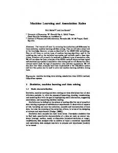
The run-time system is another area of investigation that is beyond the scope of this thesis, but it is mentioned here in order to situate the thesis within the larger project. The run-time system is an embedded MT system that uses the transfer engine to produce a lattice of partial translations. The lattice is then fed into a statistical decoder that uses an L1 language model to find the most likely path through the translation lattice. The decoder allows for reorderings of words that were translated using only the lexicon, but it does not reorder words within chunks that were produced using transfer rules. For more details on the run-time system, please refer to (Lavie et al., 2003). The system developed for this thesis is part of a larger project, the Avenue project. A system diagram of Avenue can be seen in figure 3.1 below. The idea of Avenue is to enable rapid development of MT for languages with few resources. To this end, we elicit data from bilingual speakers using a specifically designed corpus that covers a wide variety of linguistic phenomena, but is kept to minimum size because it has to be translated by an informant. The elicited data, as well as any monolingual data that may be available, is used to infer morphological information. As this module is not yet fully complete, this thesis assumes the existence of a L2 morphology module. The elicited data is further used as input to the rule learning system (this thesis). The learned rules can either be used as is, or they can go through an iterative refinement step where users (not grammar writing experts) can give feedback to the system by means of correcting translations, and the system automatically refines the learned rules based on the feedback from the user. The last step that is necessary for building a functioning system is the creation of a translation lexicon. Such lexicons are often available in some format, and can by typed up if not available in electronic form. If no translation lexicon is available, one can be built from the elicited data (of course, an existing lexicon can also be enhanced using the elicited data).

18


Figure 3.1: Avenue system diagram Finally, the learned (and refined) grammar can always be enhanced by a human expert, should one become available. Also, the learned grammar can always be enhanced if more data is translated, and can always be refined if more feedback is given. Naturally, the translation lexicon can be enhanced in a similar way. This system design allows for iterative development of the MT system such that an initial system can be built very quickly, and this initial system can be improved over time. The run-time system functions as described above: the transfer engine uses the grammar rules, the lexicon, and any available morphological information to produce a lattice of partial translations for each input sentence. The statistical decoder uses the lattice and a L1 language model to produce the most likely full translation. In order to apply our learned rules at run-time, we are often faced with the difficulty of extremely large lattices. This is especially true when using only context-free rules.1 In some cases, the lattices become so large that the transfer engine is not able to produce them, given the hardware limitations of the system it is run on. In such a case, we choose to obtain a partial lattice, which is obviously superior to not having a lattice at all. The partial lattice is produced 1 For

example, when we want to assess the quality of a set of learned context-free rules.

3.2. TRAINING DATA

19

as follows: note that the transfer engine (in its default setting) produces a full lattice of all possible partial translations, regardless of how many input words the partial translations spans. This allows us to build a partial lattice by restricting the maximum number of input indices a translation can span, thus creating a partial lattice. We build a series of partial lattices, beginning by allowing partial translations that span only one input index, then allowing partial translations that span up to two indices, etc. This approach is in the process of being replaced in the future by a beam search through the transfer engine that allows for long partial translations if they have a high score. One of the goals of chapter ?? is to assess the impact of different maximum arc lengths on the translations.

3.2

Training Data

The Avenue project targets language pairs with an unbalance in electronic resources. In particular, it is not expected that for a given language pair, a large bilingual corpus will be available. For this reason, we are designing a unilingual corpus, generally referred to as the Elicitation Corpus. The elicitation corpus is a collection of sentences and phrases in the major language (L1). Most of the designed elicitation corpus so far is in English, but part of it has been translated into Spanish, which will in particular allow us to build MT systems between Spanish and minor languages in South America (for example, Mapudungun). A native speaker of the low-density language of interest (L2) then translates the elicitation corpus into their language, and specifies the word alignments. The rule learning can proceed with an extremely small corpus: about 100 carefully selected phrases and sentences allow us to capture some major phenomena for a language pair. The elicitation corpus can thus be described as a condensed, but high-variety bilingual training corpus. In the absence of large but uncontrolled corpora, we elicit a small but controlled corpus. The elicitation corpus can be subdivided into two main parts: the functional and the structural part. The design of the elicitation corpus is not in the scope of this thesis. For coherence and focus, this thesis is aimed at using bilingual data to learn transfer rules. It is however necessary to discuss the structural elicitation corpora so as to clarify the training data that the rule learning module works with for the experiments described in this document. For further details on elicitation, the interested reader may refer to papers such as (Probst & Lavie, 2004; Probst & Levin, 2002), which deals with the corpora, their design, and their goals in greater detail.

3.2.1

Functional Elicitation Corpus

The functional elicitation corpus is designed to cover major linguistic phenomena in typologically diverse languages. The current pilot functional corpus has about 2000 sentences (in English, some of which have been translated into Spanish), though we expect it to grow to at least the number of sentences

20


in (Bouquiaux & Thomas, 1992), which includes around 6,000 to 10,000 sentences, and to ultimately cover most of the phenomena in the Comrie and Smith (Comrie & Smith, 1977) checklist for descriptive grammars. We are currently investigating techniques to create such a corpus automatically by defining comprehensive feature vectors and using a generation grammar that produces sample sentences from the feature structures that can ultimately be used for elicitation. The current corpus contains phrases and sentences such as the following: The family ate dinner. The dance amazed the children. Why are you not going to sleep? My heart beat. The linguistic features that are emphasized in this part of the corpus are features such as copula, negation, questions, passive, possessives, comparatives, numbers, etc. The most major difference between the functional and the structural corpus is that the functional elicitation corpus does not emphasize structural variation. Rather, it focuses on linguistic features. The functional elicitation corpus was designed for a multitude of purposes. For instance, it can be used to detect whether certain features exist in a language (e.g. does a language mark nouns for dual? (Probst et al., 2001)). In the future, we also envision the functional elicitation corpus to be used as input to rule learning. At this stage in development, however, the functional corpus is incomplete, and is thus not yet ready to be used for this purpose. Since a completed functional corpus would provide an ideal environment for constraint learning (as described in chapter 6), we chose to perform a case study where we use one part of the functional corpus, and learn a grammar with constraints from it. This case study deals with Hebrew copula. The copula corpus contains 287 unique elicitation examples for copula expressions, such as She was the teacher. They were students. The copula case study is described in section 6.9. For the remainder of the thesis, however, we focus on learning from the structural elicitation corpus, as explained below.

3.2.2

Structural Training Corpus

The structural part of the elicitation corpus, referred to as the structural training corpus, was designed to cover major structural phenomena. It consists of a few hundred sentences and phrases (120 structures that are exemplified with different sentences and phrases in three corpora), and it covers different make-ups of adjective phrases (ADJPs), adverb phrases (ADVPs), noun phrases (NPs), prepositional phrases (PPs), S-BARs and sentences (Ss). These types include a small number of subtypes such as SQ (a question sentence). For each of

3.2. TRAINING DATA

21

these types of structures, we have collected a number of instances of different composition. A note on VPs is in order here: in our system, we do not currently learn VPs. This is because we are mainly interested in constituent who are likely to translate into constituents of the same type. For the above constituent types, this is a safe assumption. However, VPs are different in that their make-up often changes significantly during translation. Handling VPs calls for a different approach, such as the one put forth in (Dorr et al., 2004). Beginning with a set of parses from the Brown section of the Penn Treebank (Marcus et al., 1992). The Penn Treebank is a large-scale project where different types of text were manually parsed. The parses are routinely used especially in the statistical parsing community. We mapped the Penn Treebank tagset (http://www.computing.dcu.ie/ acahill/tagset.html, ) to the tagset used by our system, and then collected statistics over the six types mentioned above. Each instance of one of these types was expressed as a pattern of expression, where a pattern is the top-node of a partial parse tree, together with the labels of the top-node’s immediate children. For example, the following two NPs are considered to be of the same pattern S→ NP VP. The jury talked. ( ( (DET the-1) (N jury-2)) ( (V talked-3))) Robert Snodgrass , state GOP chairman , said a meeting held Tuesday night in Blue Ridge brought enthusiastic responses from the audience. ( ( [Robert Snodgrass ... chairman , ]) ( [said ... audience])) We refer to the pattern of a partial parse tree as its component sequence. For each type (ADVP, ADJP, etc.), we collected a large number of different component sequences, together with their frequency of occurrence. This gave us an idea of how different structural types are expressed in English. We then created an elicitation corpus from the most frequent patterns as follows: for each type, we wanted to cover most of the probability mass of different component sequences that can express this type. For those most frequent patterns, we then either extracted or designed a generic, simple example for elicitation. Referring back to the two NP examples from above, the first example would be a better elicitation sentence, because it is simple. This will make it more likely that the sentence is actually translated to a similar structure in the other language, or else that the structure in the other language can be robustly detected automatically. The second sentence allows enough room for translation variation that the task of the rule learning system would be made much more difficult. In a postediting step, we then changed a number of lexical items so as to remain as

22


culturally unbiased as possible. This was done in part because lexical selection can cause sentences to be translated into completely different structures, and in part because this corpus is designed to be used for various language pairs, and culturally biased lexical selection can lead to sentences that are simply not translatable into many languages. During post-editing, we also eliminated a number of structures that should be elicited in the functional part of the elicitation corpus, because it is known to be expressed differently in different languages, and thus deserves special in-depth treatment. One such example is the partitive. Below we list several examples of elicitation sentences from the structural corpus: The election was conducted. the widespread interest in the election the city executive committee David can barely walk. In (Probst & Lavie, 2004) we describe a different approach to overcome the problems that lexical selection can cause. There, we makes several copies of the elicitation corpus, where in each copy the lexical items in the elicitation examples are changed. Each corpus, however, has the exact same structures. We show that lexical selection does indeed play a role in what types of structures are elicited, but that this problem can be overcome with only a small number of corpus copies. While this is an interesting and promising approach, it is not the one taken in this thesis. Rather, in the results reported here, we put the learning system in the extreme situation of having to learn from only one copy of a very small corpus. The goal was to determine what we can learn under those severe circumstances. If we can learn meaningful rules and improve translation quality, we show that the approach put forth in this thesis can really be applied to language pairs where we can obtain only very little data. The structural elicitation corpus consisting of 120 sentences and phrases was translated and aligned for both Hebrew and Hindi. Unless otherwise noted, all learned grammars that are described in this document were learned from the structural corpus.

3.2.3

Training Data Format

During elicitation, the bilingual informants provides the translation of an elicitation example as well as word-level alignments. In addition, the rule learner is given the English parse of each training example. In the case of the structural training corpus, the parse is the parse from the Penn Treebank (with possible small changes if the lexical items were changed from the original sentence in the Penn Treebank to the sentence used in the structural corpus). For the functional corpus, we used the Charniak parser (Charniak, 1999). As all the training examples in the functional corpus are very short and structurally simple sentences, the Charniak parser yields very reliable results.

3.2. TRAINING DATA

23

In addition to a translation pair, word alignments, and the English parse, each training example also contains type information as well as a co-embedding score. The type is the label of the top-node of English parse of each example. The co-embedding score essentially captures the depth of the parse tree. It will be described in more detail in chapter 5, as it is used during compositionality learning. Type and co-embedding scores can be obtained off-line before learning. This results in improved efficiency of the rule learner. All rule learning training data is tagged with co-embedding scores and type information for this reason. A complete training example then looks as follows: SL: in the forest TL: B H I&R Alignment:((1,1),(2,2),(3,3)) Type: PP CoEmbeddingScore: 3 C-Structure:( (PREP in-1)( (DET the-2)(N forest-3)))

3.2.4

A Note on Uncontrolled Corpora

The rule learning techniques developed in this thesis are not aimed specifically at the controlled elicitation corpora described in the previous sections. In fact, the rule learning module could be run just as easily on any bilingual data that is available, with automatically assigned word alignments. We have developed some techniques to learn under a variety of circumstances, such as from uncontrolled corpora and from automatically induced L2 morphology modules. (Probst, 2003) However, this is not the main line of this research. The goal of this thesis was to investigate what can be learned under a a miserly data scenario, for example from only the structural elicitation corpus of 120 sentences. As mentioned above, if we can learn meaningful grammars from a corpus this small, we can make a strong case that our approach can be applied to language pairs where very little data is available. Learning from uncontrolled corpora is a very exciting and promising direction that this research could take in the future. It is however an equally big project to the one described in this thesis. For the purposes of this thesis, this problem is considered to be out of scope.

3.2.5

Evaluation Methodology

Throughout the thesis, the learned grammars are evaluated in two ways: first by a discussion of the learned rules and their application, and second in a ‘task-based’ evaluation where the rules are used in the context of a translation system. The discussion of the learned rules is both useful and important, as the goal of the thesis is to emulate a human grammar writer. If the rule learning module can automatically infer rules that are like rules that a human grammar writer would write, then the goal is accomplished. For each module, and each substantial learning phase, we thus discuss the learned rules and their strengths

24


and weaknesses. We also demonstrate how the learned rules in a specific module accomplish the goal of this module. For example, if a module is designed to solve the problem of pro-drop, we demonstrate how the learned rules capture pro-drop and improve translation quality. In the task-based evaluation, the grammar is used with the transfer engine to produce a lattice, and the decoder is used to produce a final translation. The translations are evaluated with automated evaluation techniques. We use BLEU (Papineni et al., 2001), a slightly modified version of BLEU called modified BLEU or ModBLEU that uses the arithmetic rather than the geometric average over n-gram matches and thus does not produce a score of 0 if no highern-grams are matched, and finally the METEOR metric (Lavie & Sagae, 2004). It is important to note that BLEU and ModBLEU put a stronger emphasis on precision than on recall, whereas METEOR puts more emphasis on recall. Interestingly enough, this basic difference is consistently observed in our results. For example, whenever an algorithm is designed to improve recall while sacrificing some precision, the METEOR score generally increases, while the BLEU and ModBLEU scores decrease. In addition to the translation evaluation metrics, we also use a Lattice Evaluation, which abstracts away from the decoder: it evaluates the lattice produced by the transfer engine by comparing it to the reference translation(s) much in same way as BLEU and METEOR do. The lattice evaluation compares the translation chunk of each lattice arc against the reference translation. It first counts the number of unigrams, then the number of bigrams, etc. up to a specified maximum n-gram size. For each match, the arc’s score is increased. The lattice scoring also takes into account the length of the arc, and how many times each of the matched n-grams was already matched in a given sentence. If an arc contains an n-gram match that was already proposed by another arc, then the addition to the arc score is discounted based on how many times the matched n-gram was already observed. In this way, an arc receives a boost in score for each matched n-gram. However, frequently matched n-grams are not rewarded as highly, because an arc that contains a frequently matched n-gram adds very little to the quality of the lattice. Multiple reference translations are handled by computing the score for an arc for each reference translation, and then retaining only the maximum value. Since the evaluation method is not directly part of the thesis, more details can be found in the appendix under section A. In the work reported here, the lattice evaluation metric is used to assess the quality of individual rules. We can measure how well rules perform (independently of the decoder) by evaluating the quality of the arcs that were produced using this rule. More details on rule scoring can be found in section ??. We report results for each individual learning phase and each training set, and compare the results. In addition to comparing different grammars, we also compare the learned grammars to a baseline and a manually written grammar. The baseline is a translation without a grammar, but only with the statistical decoder and the lexicon. The manually written a Hebrew→English grammar that was designed by a human expert within the course of about a month. While not comprehensive, this grammar can be seen as a gold standard of sorts: the

3.2. TRAINING DATA

25

goal of the thesis is to learn rules that are as similar to hand-written rules as possible, thereby emulating a human grammar writer. The experiments were performed on a development set of 26 parallel sentences of newspaper style text. In addition, we evaluate the algorithms on an unseen test set of 62 sentences, which are again newspaper test. We further evaluated on a test suite that targets specific syntactic phenomena of interest, for instance reordering of adjectives and nouns between Hebrew and English. The test suite has 138 sentences. The test suite and the evaluation on it will be discussed in section 7.6. The run-time system is generally used in a mode that allows the user to specify the maximum arc length of partial translations. For example, a length limit of 6 means that the maximum number of source indices that can be spanned by any one arc is 6. While this is suboptimal in the sense that we do not obtain complete lattices, the length limit is a very useful tool in practice. It is set in order to combat the often very large number of possible arcs. The decoder chooses between the possible partial translations, but when there are sufficiently many partial translations, the transfer engine is not able to produce all of them. Unless otherwise specified, we report results throughout for a length limit of 6. In section 7.8, we compare the performance of grammars under different length limits.

26


Chapter 4

Seed Generation 4.1

Introduction

Seed Generation is the process of building initial transfer rules from the training data. This is done using the parses, the dictionary, and, if applicable, a morphology module for the minority language L2. The goal of this module is to produce completely flat rules. This means that the component sequences contain only lexical items and/or parts of speech. Non-terminals such as NPs are introduced during compositionality learning. These elements will allow rules to apply in combination. Flat seed rules can only apply individually to unseen text. Further, they are generally highly lexicalized: with few exceptions, any word that is not aligned one-to-one is left lexicalized during Seed Generation. Compositionality learning overcomes this one-to-one restriction for many cases. Seed generation, like all other learning modules, learn rules only for a set of relevant types. The relevant types for the Hebrew→English were determined to be ADVP, ADJP, NP, PP, SBar, and S. Other non-terminals, in particular VP, are very difficult to capture in transfer mappings, because they are more likely exhibit structural mismatches. Since our rules are learned completely automatically, excluding VPs from our choice of relevant types is merely a conservative precaution. This does not mean that VPs are not an integral part of the learned rules, but no sequence of parts of speech and/or non-terminals is ever generalized to a VP, and no rule exists that is of type VP::VP.

4.2

Description of Learning Algorithm

Seed Generation processes each training example in turn. For each training example, it constructs an initial transfer rule called a seed rule, if certain conditions are met. The seed rule is a complete transfer rule in format: it contains L1 and L2 type information, component sequences, and alignments. In other words, it is a fully functional transfer rule. Seed rules are initially produced in 27

28

CHAPTER 4. SEED GENERATION

Seed Generation for all training examples for all 1-1 aligned words get the L1 POS tag from the parse get the L2 POS tag from the morphology module and the dictionary if the L1 POS and the L2 POS tags are not the same, leave both words lexicalized for all other words leave the words lexicalized Figure 4.1: Pseudocode for Seed Generation the direction L1→L2, because for a normal system run they are immediately fed into compositionality learning, which is done in this direction. They can however also be output as complete learned rules, in which case the direction is flipped before outputting. For each training example, the task of the seed generation module is to produce the following rule parts: • L1 type information • L2 type information • L1 component sequence • L2 component sequence • word-level alignments In figure 4.1, we present the Seed Generation algorithm in pseudocode. While it is not possible to include all details in the pseudocode listing, it can be useful for giving an overview picture. The L1 type information is obtained from the parse, it is simply the label of the top node. The L2 type information is assumed to be always the same as for the major language, so that the L1 type information in each seed rule is also the parse’s top node. This approach comes from the underlying assumption that elicitation targets those sentence components that are likely to transfer into the same kind of component, e.g. noun phrases are assumed to translate into noun phrases. The L1 component sequence can essentially be obtained from the parse: for each word in the training example’s L1 sentence or phrase, the part of speech of this word can be looked up in the parse. One restriction that is put on

4.3. RESULTS

29

the component sequences is that only words that are aligned one-to-one can be represented by their POS in the component sequence. By contrast, non-one-toone aligned words are left lexicalized, i.e. the lexical item from the translation sentence remains in the component sequence. L1 component sequences are obtained similarly to their L1 counterparts. Any one-to-one aligned word is potentially replaced by a POS label. As the rule learning system works without an L2 parse, the bilingual dictionary is used to form a better estimate of what the POS of a given L2 word should be. For all one-to-one aligned words, the L1-L2 word combination is first looked up in the dictionary. In is not found, it is assumed (in the absence of any other information) that the L2 POS label is the same as the POS of the corresponding L1 word. Both the L1 and L2 word will be replaced by their parts of speech in the learned seed rule. Similarly, if the L1-L2 word combination is found in the dictionary and the dictionary entry’s L1 POS is the same as the L1 word’s POS in the parse, the words are raised to the POS level. However, if the L2 part of speech is not the same, then both the L1 word and the L2 word are being left lexicalized. If a word is not aligned one-to-one, it must remain lexicalized. In the Hebrew→English case, the dictionary is in full form for English, but in root form for Hebrew. Therefore it is necessary that the rules contain Hebrew lexical items in their root form if the words are to remain lexicalized. The root form can be obtained as follows: the Hebrew word is analyzed by the Hebrew morphology module, which returns a list of possible roots. Each root and all possible English translations from the training example are then looked up in the dictionary. If there exists an entry for such a combination, then the proposed root is returned as the root for the given L2 word. If no such entry exists, but the morphology module returns exactly one possible root, then this root is returned. If a root is found, the root is entered into the L2 component sequence instead of the original word. If not, then the original Hebrew lexical item is entered into the L2 component sequence. As was mentioned above, the seed generation module produces completely ‘flat’ rules. This is done in practice by allowing the component sequences to contain only literals and parts of speech, i.e. only components that refer to at most one word in the training examples. Components that can span more than one word, and can be filled by other grammar rules, are learned during compositionality.

4.3 4.3.1

Results Discussion of Learned Rules

We will now discuss some rules for Hebrew→English translation that were learned using only the seed generation module. As mentioned above, all rules were learned from the structural elicitation corpus, which consists of 120 sentences and phrases.

30

CHAPTER 4. SEED GENERATION

Note that some lines in the rules are preceded by a semicolon. These lines are ignored by the transfer engine. For instance, the original training examples are given in the rules merely as a mnemonic for the human reader. Similarly, alignments that are not 1-1 are still indicated in the rule, again to make the rule easier to read. These alignments are disallowed by the transfer engine, so they must be commented out. ;;L2: $MX MAWD &L H XD$WT ;;L1: VERY HAPPY ABOUT THE NEWS ;;C-Structure:( ( (ADV very-1))(ADJ happy-2) ( (PREP about-3)( (DET the-4)(N news-5)))) ADJP::ADJP [ADJ ADV PREP DET N] -> [ADV ADJ PREP DET N] ( (X1::Y2) (X2::Y1) (X3::Y3) (X4::Y4) (X5::Y5) ) This rule is a good example of a rule that captures an interesting structure. It was learned that the English pre-adjectival adverb appears after the adjective in Hebrew. The position of the prepositional phrase is the same for both languages. Note that this rule does not contain any lexicalized items, as all words very aligned one-to-one. A rule such as this first example will readily apply to unseen text. ;;L2: H QBWCH H XD$H $LW ;;L1: HIS NEW TEAM ;;C-Structure:( (POSS his-1)(ADJ new-2)(N team-3)) NP::NP ["H" N "H" ADJ POSS] -> [POSS ADJ N] ( (X2::Y3) (X4::Y2) (X5::Y1) ) This rule expresses how simple possessives, in conjunction with an adjective, are realized in Hebrew. It was learned that while an English NP with a possessive, as in the example, generally does not mark for definiteness, the Hebrew definiteness marker ”H” appears on both the noun and the adjective. It should also be noted that the entire phrase is completely reordered in Hebrew. ;;L2: KL KK XZQ $ HIA $KXH ;;L1: SO INTENSE THAT SHE FORGOT ;;C-Structure:( ( ( (ADV so-1))(ADJ intense-2)) ( (SUBORD that-3)( ( (PRO she-4))( (V forgot-5)))))

4.3. RESULTS

31

ADJP::ADJP ["KL" "KK" ADJ SUBORD PRO V] -> ["SO" ADJ SUBORD PRO V] ( ;--;(X1::Y1) ;--;(X2::Y1) (X3::Y2) (X4::Y3) (X5::Y4) (X6::Y5) ) This is an example of a partially lexicalized rule that nevertheless captures an interesting Hebrew expression and its English counterpart. The English intensifier ”SO” is expressed in Hebrew as the two words ”KL” ”KK”. The words remained lexicalized during learning because they were not aligned one-toone. Advanced compositionality learning will aim at overcoming this limitation; in its current state, this rule, albeit interesting, will apply to very few test examples because of its partial lexicalization. Finally, we present an interesting example of reordering of noun compounds between Hebrew and English. ;;L2: TKNIT H @IPWL H HTNDBWTIT ;;L1: THE VOLUNTARY CARE PLAN ;;C-Structure:( (DET the-1)( (ADJ voluntary-2)) (N care-3)(N plan-4)) NP::NP [N "H" N "H" ADJ] -> ["THE" ADJ N N] ( (X1::Y4) ;--;(X2::Y1) (X3::Y3) ;--;(X4::Y1) (X5::Y2) As previously, the determiner in Hebrew appears more than once. In Hebrew, noun compounds mark definiteness only on the second noun. The determiner is repeated on the adjective.

4.3.2

Automatic Evaluation Results

Seed generation was run on the Clean Structural Corpus.For each learned grammar, we computed several automated evaluation scores. We report here the BLEU score, the ModBLEU score, as well as the METEOR score (Lavie & Sagae, 2004). Here and for the remainder of the document, we compare against a baseline translation without a grammar and a translation with a hand-written grammar. Table 4.1 presents the results for the baseline without a grammar, manually written grammar, and the grammars that were learned from the structural

32

CHAPTER 4. SEED GENERATION Grammar No Grammar Manual Grammar Learned Grammar (SeedGen)

BLEU 0.0255 0.0713 0.0281

ModBLEU 0.0910 0.1209 0.0969

METEOR 0.2681 0.3204 0.2786

Table 4.1: Seed Generation Only Evaluation Results.

corpus. It can be seen from the automated evaluation results that a some improvement of translation quality can be gained from the flat seed rules alone. This indicates that the seed rules capture the kinds of structural phenomena that are targeted during learning. It also indicates that the rules can generalize beyond the training sentences they were inferred from, and can be used to translate unseen examples. Under this comparison, the manual grammar outperforms the learned grammar noticeably. The goal of the more advanced learning phases is then to improve upon the performance of the seed rules, and to get as close as possible or beyond the performance of the manual grammar.

Chapter 5

Structural Learning 5.1

Introduction

The previous chapter described the Seed Generation algorithm, during which a set of rules are learned that closely reflect the training data. In this and and the following chapter, we shift our attention to learning more complex rules, i.e. rules that generalize further over the training data, and that capture higher-level structure as well as context. The problem of learning complex transfer rules can be subdivided into two main sections: learning structure, and learning unification constraints. This chapter addresses the first of these issues, the learning of structural mappings. Why are structural mappings important? They allow us to reorder not only words, but also entire constituents. They also allow us to capture in part the structure of the minor language L2. As mentioned in the related work section (section 3), a very important distinction between our work and a body of recent related work is that in our framework, we do not assume the availability of an L2 parser. This makes the learning of structures all the more challenging. This chapter provides an in-depth discussion of learning structure with only a parser for the major language: it discusses what is learnable, and proposes learning algorithms for those structures that can be learned in our framework. The proposed algorithms are only one possible approach to learning the structures that can be learned. Other groups may find it useful to take the discussion on what structures are learnable as a starting point for their own investigation.

5.2

Taxonomy of Structural Mappings

In this section, we discuss the theory of what structures can exist, and what structures are learnable. There are several factors to consider: 1. The space of possible mappings 2. The space defined by the rule formalism 33

34

CHAPTER 5. STRUCTURAL LEARNING 3. The space defined by the learning algorithm

The following sections will provide discussions of each of these spaces. In particular. We will discuss the advantages and disadvantages of the rule formalism. We will then derive an argument of what the learning algorithms address and why. Our goal is to at least address in discussion all important types of mappings; in the case of structural mappings that are not learnable by our algorithms, we give a discussion of why this is the case. Some issues are left for future work. The goal of this section is to give a comprehensive discussion of the structural learning problem. Before discussing the three spaces within which the learning system resides, we give a listing of the specific constraints on our system that do not influence the generality of the argument following it.

5.2.1

System Constraints

In this section, we lay out a set of constraints under which our system must work. The constraints are meant to not influence the generality of the approach. Instead, they make the discussion feasible by making it concrete. We apply the following constraints: 1. Mappings are applied at most at the sentence level. Each mapping (rule) captures a transformation of a phrasal instance or a complete sentence, but not a paragraph. 2. The transfer rules are designed to be unidirectional from the minor language (L2) to the major language (L1). 3. The rules must be learned under the resource constraints described in previous chapters, in particular the availability of a parser only for the major language. Due to these restrictions, the structural part of the rules are highly dependent on the L1 parse information.

5.2.2

General Space of Possible Mappings

The general space of structural mappings can be regarded as any mapping between the two languages. The most specific mapping is between two completely lexicalized sentences. This is not a structural mapping, because it does not provide any generalization power: no other (partial) sentences can be translated with such a mapping. Further, the mapping is flat, thus does not provide any hierarchy. Example-based machine translation operates mostly at this level. The work developed in this thesis uses the completely lexicalized level as the specific boundary while aiming at inferring more structural mappings, meaning that they will 1) generalize to unseen examples, i.e. abstract away from the lexical level as much as possible, and 2) provide a hierarchical structure, i.e. mapping (partial) trees of structures. Completely lexicalized mappings clearly form the specific boundary of our work. The general boundary is not as intuitively found without delving into the

5.2. TAXONOMY OF STRUCTURAL MAPPINGS

35

specifics of our approach, which is not the goal of this section. We will define the general boundary of possible mappings as any mapping that abstracts away from lexical items by introducing categories (such as parts of speech or constituents, or even non-linguistically defined categories). This provides a vast space, but it gives a first approximation to framing the learning problem.

5.2.3

Space Defined by Rule Formalism

Before learning structural mappings, it is necessary to define a set of tags that describe categories of words or or higher-level structures. The rule formalism developed for this work allows for two types of categories in addition to lexical items. The categories are as follows: 1. Non-terminals (NT): non-terminals are used in two rule parts: first, in the type definition of a rule (both for SL and TL, meaning X0 and Y0), and second in the constituent sequences for both languages. Non-terminals can be defined as any label that can be the type of a rule. They describe higherlevel structures such as sentences (S), noun phrases (NP), or prepositional phrases (PP). Generally, they can be filled with more than one word. In other words, NTs in constituent sequences are filled by other rules. 2. Pre-terminals (PT): pre-terminals can only be used in the constituent sequences of the rules, and not as X0 or Y0 types. As a principle, they can be filled with only one word.1 Pre-terminals are filled by lexical entries, not by other grammar rules. 3. Terminals (LIT): terminals are lexicalized entries in the constituent sequences, and can be used on both the x- and the y-side. They can only be filled by the specified terminal itself. These categories in combination with the definition of the rule formalism narrow the space of possible rules that can be learned. They enforces that there is a hierarchy of levels of abstraction, as specified by the categories. The rule formalism furthermore implies a number of restrictions on the types of rules that the transfer engine can translate. Note that these restrictions are independent of any restrictions imposed by the learning algorithms on what rules could be learned from data. In fact, many rules could be learned, but could not be used for run-time translation, because they are meaningless in our system. This will become clearer further along in the discussion. The restrictions imposed by the rule formalism are subtle, but have wide-reaching implications. They are as follows: NTs must not be aligned 1-0 or 0-1. Proof by contradiction: Suppose NTs could be aligned 1-0 or 0-1. 1 There is one exception to this principle, which is the case where a lexical entry is a phrasal entry (i.e. it has more than one word). This exception is however not relevant to the present discussion.

36

CHAPTER 5. STRUCTURAL LEARNING • Case 1: 1-0 alignment: Consider the following (abstract) rule that contains a 1-0 alignment of an NT:

NT1::NT1 [PT1 NT2] -> [PT1] ((X1::Y1)) This rule may at first glance seem like a meaningful rule. Note, however, that it can never be applied. In order to resolve (fill) NT2 with actual words, it would need to apply another grammar rule with NT2 as its xside type and no y-side type (as NT2 does not align to anything). The rule formalism enforces that each grammar rule must have an x-side and a y-side type. Hence, this rule can never resolve the NT2 and can thus never apply to produce a translation. q.e.d. • Case 2: 0-1 alignment: The same argument as for case 1 holds here, the only difference being that the grammar would need to contain a rule without a x-side type. The rule formalism does not allow this, hence a 0-1 alignment is impossible. q.e.d. A similar argument can be made for PTs: PTs must not be aligned 1-0 or 0-1. Proof by contradiction: • Case 1: 1-0 alignment: Consider the following ( abstract) rule that contains a 1-0 alignment of an PT:

PT1::PT1 [PT2 NT1] -> [NT1] ((X2::Y1)) In order for this rule to apply, there would need to be a lexicon entry with PT2 as its x-side top-node, but without a y-side top-node. This is not allowed in the transfer rule formalism, so that such a rule cannot exist in the lexicon, and the above rule can never apply. q.e.d. • Case 2: 0-1 alignment: Finally, a 0-1 alignment for a PT is equally impossible. It would require a lexicon entry with an empty x-side top-node, which is not allowed in the transfer rule formalism. Thus, a rule with a 0-1 alignment for a PT can never apply. q.e.d. In practice, unaligned PTs result in undefined transfer engine behavior and should thus never occur in any rules.


37

Any word in the bilingual training pair must participate in exactly one LIT, PT, or NT. Proof: This principle follows from the fact that the transfer engine matches against the input linearly. If a word participated in more than on LIT, PT, or NT, the transfer engine could either not apply the rule because it would not match the input, or else it would produce some words multiple times, both of which are clearly undesired effects. q.e.d. Although these principles limit the space of meaningful rules, we have not yet developed a clear picture of what kinds of structures are possible in the given transfer rule formalism. In order to obtain a more complete picture, the space of possible rules can be expressed as a set of transformations, as follows: 1. Transformation I. The X0 node, i.e. the top-level node for the x-side, is transformed into the x-side constituent sequence. 2. Transformation II. The X0 node, i.e. the top-level node for the x-side, is transformed into the Y0 node, i.e. the top-level node for the y-side. 3. Transformation III. The Y0 node, i.e. the top-level node for the y-side, is transformed into the y-side constituent sequence. 4. Transformation IV. The x-side constituent sequence is transformed into the y-side constituent sequence. It is not immediately obvious why these four transformations do in fact capture the entire space of possible transfer rules under the rule formalism, so we will discuss why this is the case. In principle, the first two transformations are exactly the language defined by a context-free grammar that transforms the top nodes into productions (or component sequences, as they are referred to in our formalism). The first transformation captures what x-side constituent sequences can be produced from the X0 node, the second transformation captures what y-side constituent sequences can be produced from the Y0 node. The first and third transformations would be enough to capture the entire space of possible mappings, were it not for the fact that the x-side and y-side are by no means independent. In fact, each transfer rule is tied to the other language by transformations II and IV: these transformation captures what structures can possibly occur together in one specific rule. For example, in the previous section we have proven that it is not possible for NTs or PTs to be aligned to the empty word. These kinds of restrictions can only be captured via transformations II and IV between the x-side and the y-side. We can now describe the four above transformations in terms of the categories described above (NTs, PTs, LITs), as well as an additional empty word, ǫ. • Transformation I. – NT → (NT | PT | LIT)+

38

CHAPTER 5. STRUCTURAL LEARNING • Transformation II. – NT → NT • Transformation III. – NT → (NT | PT | LIT)+ • Transformation IV. – NT → NT+ – PT → PT+ – LIT → ǫ – ǫ → LIT LITs are always considered unaligned by the transfer engine.

Any learning algorithm that we design must stay within the parameters of what the transfer formalism allows. Otherwise, we would get rules that would be meaningless to the transfer engine, as explained above. In the following settings, we will frame the learning algorithm within these constraints.

5.2.4

Space Defined by Learning Setting

The rule formalism imposes certain constraints on what rules can be handled. Similarly, the learning setting imposes a set of constraints. For convenience, we summarize below in one list what has been said in various places above. The learning setting makes the following assumptions: 1. The presence of an L1 parser. 2. The absence of an L2 parser. 3. Word alignments are given for the training data. 4. We define the set of non-terminals, i.e. the types of rules that can be learned, as the set NT. In our system, NT consists of ADVP, ADJP, NP, PP, SBAR, and S (with a few subtypes such as SQ that do not have significant impact on the present discussion). The assumption with the strongest implications is the absence of an L2 parser. For this reason, we generally assume that an L1 NT translates into the same NT on the L2 side. So for example, since we only have a parser for the major language (L1), we assume that an NP will translate into an NP on the other side.

An L1 NT is assumed to translate into the same NT in L2.


39

This assumption has wide-reaching implications, as it restricts the types of structures that can be learned. This simplifies learning, but it also limits the system. Folding the above assumption into the four transformations yields the following: • Transformation I. – NT → (NT | PT | LIT)+ (unchanged) • Transformation II. – N Ti → N Ti (same type of NT) • Transformation III. – NT → (NT | PT | LIT)+ (unchanged) • Transformation IV. – – – –

N Ti → N Ti + (same type of NT) PT → PT+ (unchanged) LIT → ǫ (unchanged) ǫ → LIT (unchanged)

Closer inspection of these transformations shows that the first and third transformation do not pose any real restrictions on the rule learning algorithm. The only restriction is that at least one index must be produced, but this index can be filled by a LIT, PT, or NT. Transformation I, on the other hand, is now quite restrictive. Future work will address the softening of the assumption of direct transfer of NTs. Transformations II and IV can be viewed as expressing cross-lingual learning. Let this be called ‘xy learning’. Further, consider the categories NT, PT, and LIT in a hierarchy where NT is the highest-level and LIT is the lowest-level category. Finally, let a ‘sequence’ be defined as one or more instances of one category. Then a closer inspection of Transformations II and IV allows us to postulate the following axioms: 1. A NT cannot map down. A NT must map to another NT of the same type. It cannot map to a sequence of PTs or LITs, and it cannot map to the empty word ǫ. 2. A PT cannot map up down. A PT cannot map to a sequence of LITs, and it cannot map to the empty word ǫ. Correlary of axiom 1: A PT cannot map up. It cannot map to a sequence of NTs. 3. A LIT can map to the empty word ǫ, and the empty word ǫ can map to a LIT. Literals can only map to the empty word ǫ2 . Correlary of axioms 1 and 2: A LIT cannot map up. 2 Remember

that literals are always considered unaligned by the transfer engine.

40

CHAPTER 5. STRUCTURAL LEARNING

Furthermore, the above discussion leads us to the following additional axiom. Although this was discussed above, it should be repeated here as an axioms, as all learned rules must abide by these axioms: 4. Any word must participate in exactly one LIT, PT, or NT. This follows from the fact that the transfer engine matches against the input linearly. See section 5.2.3 for a more detailed discussion. These axioms stem from a combination of a) the transfer rule formalism and transfer mechanism and b) the restrictions imposed in the absence of the transfer engine. In fact, we could easily design a learning algorithm that would propose rules that violate these axioms, but the system will never be able to apply them properly. Therefore, any learning algorithm must either be designed to never violate these axioms, or else must filter out all learned rules that violate one or more of the axioms, because such rules will merely slow the system without any added benefit. The question then becomes how to define a learning mechanism that will learn reasonable structures while at the same time ‘playing’ within the rules of the game, i.e. not violating any of the axioms. In the sections it will become clear how our learning algorithms ensure that all learned rules abide by the axioms.

5.3

The Basic Compositionality algorithm

In order to exploit the inherent structure in the training examples, and in order to scale better to unseen examples, the system learns compositional rules. The goal of this module is to learn the context-free backbone of the transfer grammar. This is achieved by traversing the L1 parse from the top-down, and introducing a compositional element for a subnode wherever appropriate. Two basic settings are possible for compositionality learning: assuming maximum compositionality, or using the transfer engine and previously learned rules to decide whether compositional elements should be introduced. We will discuss these settings in the following two sections. This section lays out the algorithm independently of the maximum compositionality parameter. Consider the following training example and the corresponding seed rule as generated by the learning module: SL: a year later they returned TL: $NH MAWXR IWTR HM $BW Alignment: ((2,1),(3,2),(3,3),(4,4),(5,5)) Type: S CoEmbeddingScore: 4 C-Structure: ( ( ( (DET a-1)(N year-2)) (ADV later-3)) ( ( (PRO they-4))

5.3. THE BASIC COMPOSITIONALITY ALGORITHM

41

( (V returned-5)))) ;;L1: A YEAR LATER THEY RETURNED ;;L2: $NH MAWXR IWTR HM $BW S::S ["A" N "LATER" PRO V] -> [N "MAWXR" "IWTR" PRO V] ( (X2::Y1) ;--;(X3::Y2) ;--;(X3::Y3) (X4::Y4) (X5::Y5) ) The seed rule is flat, as desired by the basic seed rule algorithm. In order for this rule to scale to a larger number of test sentences, several generalizations of the seed rule are possible: ;;L1: A YEAR LATER THEY RETURNED ;;L2: $NH MAWXR IWTR HM $BW S::S ["A" N "LATER" PRO VP] -> [N "MAWXR" "IWTR" PRO VP] ( (X2::Y1) ;--;(X3::Y2) ;--;(X3::Y3) (X4::Y4) (X5::Y5) ) ;;L1: A YEAR LATER THEY RETURNED ;;L2: $NH MAWXR IWTR HM $BW S::S ["A" N "LATER" NP V] -> [N "MAWXR" "IWTR" NP V] ( (X2::Y1) ;--;(X3::Y2) ;--;(X3::Y3) (X4::Y4) (X5::Y5) ) ;;L1: A YEAR LATER THEY RETURNED ;;L2: $NH MAWXR IWTR HM $BW S::S [ADVP PRO V] -> [ADVP PRO V] ( (X1::Y1) (X2::Y2) (X3::Y3) )

42


;;L1: A YEAR LATER THEY RETURNED ;;L2: $NH MAWXR IWTR HM $BW S::S ["A" N "LATER" S] -> [N "MAWXR" "IWTR" S] ( (X2::Y1) ;--;(X3::Y2) ;--;(X3::Y3) (X4::Y4) ) ;;L1: A YEAR LATER THEY RETURNED ;;L2: $NH MAWXR IWTR HM $BW S::S [ADVP S] -> [ADVP S] ( (X1::Y1) (X2::Y2) ) These rules are of varying degrees of generality. More specifically, the last rule is the most general rule. This means that it will apply to a large number of unseen examples, while at the same time generalizing away from the specific training example in the best possible way. One of the most basic problems that we are facing when learning transfer rules is the trade-off between scaling to unseen examples and overly general rules that apply in many contexts where they should not apply. All of the algorithms described in this thesis attempt to strike a balance between those two competing scenarios. On the one hand, we want to generalize beyond the training data. On the other hand, it happens frequently that a grammar contains a small number of ‘bad’ rules, i.e. rules that apply to too many contexts. The goal of compositionality is essentially to create very general rules that will apply to a variety of new contexts. By contrast, the unification constraints serve to limit the applicability and/or output of the rules. In this way, compositionality and constraint learning together serve to strike an appropriate balance, as supported by the training data. How can we learn a compositional rule such as the ones listed above from the seed rule? This can be accomplished by traversing the L1 parse from the top down. For each subnode, the algorithm decides whether or not to introduce a compositional element. This decision depends first on whether maximum compositionality is assumed or not. It further depends on subtle issues such as whether the L1 component aligns to a coherent set of L2 words, or whether the aligned L2 words align to other L1 components. These advanced issues will be described below. The algorithm will first try to introduce a compositional element for each of the direct children of the root. The root itself is not considered for compositionality, because we do not want to introduce completely recursive rules of the form S::S [S] -> [S]

5.4. APPROACH I: LEARNING WITHOUT ASSUMING MAXIMUM COMPOSITIONALITY43 ( (X1::Y1) ) Such rules do not add any new information to the grammar, and will make the run-time infinite by applying repeatedly. For each direct child of the node, a compositional element can be introduced. If this happens, no further traversal of the subtree rooted at the child takes place. Otherwise, the compositionality algorithm descends further into the tree, with a base case of leaving the seed rule non-compositional. What exactly does it mean to introduce a compositional element? The label of the compositional subroot is inserted into the component sequences (in the appropriate place) of the rule. As was discussed above, we always require that the label of a compositional element is the same both for the L2 and L1. This is necessary so that other rules can ‘plug into’ the now compositional rule. For example, if a compositional element is of the type NP, then this NP can be resolved at run-time using another NP::NP rule, as in a standard context-free grammar. Since the compositionality algorithm traverses the parse from the top-down, it prefers the most far-reaching compositional elements. For instance, if the S ‘they returned’ qualifies for compositionality, then the lower-level NP ‘they’ is no longer even considered for compositionality. This again illustrates the fact that compositionality aims at learning rules that are as general as possible while still supported by the training data. In figure 5.1, we present the basic compositionality algorithm in pseudocode. As will be explained in greater detail below, whether compositionality is valid for a given subroot depends in part on whether maximum compositionality is assumed or not. If maximum compositionality is assumed, compositionality is always assumed valid; if not, then compositionality is only valid if a previously learned rule can translate the L1 sequence that the subroot spans into the corresponding L2 sequence.

5.4

Approach I: Learning without assuming maximum compositionality

In the learning setting where maximum compositionality is not assumed, the rule learner uses previously learned rules to determine whether or not a compositional element should be introduced. Note that under this paradigm, it is very important what order the rules are learned in. Sections 5.4.1 and 5.4.2 discuss how the appropriate order can be ensured. How can the rule learner use previously learned rules to determine whether a compositional element should be introduced? First, each of the nodes in the parse is used to a) extract the L1 substring (w1,L1 . . . wk,L1 in the pseudocode above) covered by this node b) using the alignments, create a L2 substring

44


Basic Compositionality Algorithm IntroduceCompositionalElement(Root), where Root is the root of the L1 parse IntroduceCompositionalElement(Subroot) get parse label labelSubroot of Subroot extract w1,L1 . . . wk,L1 covered by Subroot extract w1,L2 . . . wl,L2 aligned to w1,L1 . . . wk,L1 if w1,L2 . . . wl,L2 contiguous and w1,L2 . . . wl,L2 6= ǫ if compositionality valid for Subroot Replace w1,L1 . . . wk,L1 by labelSubroot in the rule Replace w1,L2 . . . wl,L2 by labelSubroot in the rule Adjust the alignments in the rule else for each child of Subroot Childi,Subroot , i ≤ m, where m is the number of children of Subroot IntroduceCompositionalElement(Childi,Subroot) else for each child of Subroot Childi,Subroot , i ≤ where m is the number of children of Subroot IntroduceCompositionalElement(Childi,Subroot) Figure 5.1: Pseudocode for Basic Compositionality

m,

5.4. APPROACH I: LEARNING WITHOUT ASSUMING MAXIMUM COMPOSITIONALITY45 corresponding to the L1 chunk (w1,L2 . . . wl,L2 above), c) the type of the node (labelSubroot). The learning algorithm then uses all rules of type labelSubroot to translate the L1 chunk that was extracted from the training example. Only rules of this type can serve as the top-node in this translation. The rules can however combine with rules of any other type to form a translation of w1,L1 . . . wk,L1 . If any of the possible translations is the correct translation w1,L2 . . . wl,L2 , then a compositional element can be introduced if w1,L2 . . . wl,L2 is contiguous. To return to the previous example, consider the node and subtree ( ( (PRO they-4)) ( (V returned-5)))) The compositionality algorithm then extracts the L1 chunk ’they returned’ and, using the alignments, the L2 chunk ‘HM $BW’. Then the transfer engine uses all previously learned rules of type S to translate ‘they returned’. If one of the possible translations is the expected ‘HM $BW’, a compositional element is introduced with the label ‘S’ both for L1 and L2. Finding a correct translation for the L1 chunk means that we have previously learned a rule of type S which, possibly in combination with other previously learned rules, can translate this chunk. Two exceptions hold: first, the L2 chunk must be contiguous, and second, a compositional element is not introduced when the L1 constituent is not aligned to any word in L2. In this case, it is safer to simply leave this sequence lexicalized3 . What are the previously learned rules? Rules are learned in several iterations according to their co-embedding score and type, as will be described below (sections 5.4.1 and 5.4.2). As before, compositionality begins from the top of the parse and therefore introduces compositional elements that are as big as possible. The advantage of this approach is that we only introduce compositional elements that are warranted by the previously learned rules and thus is directly ‘endorsed’ by the training data. The disadvantage is that there is a strong reliance on structural variety in the training data: if a certain structure was not encountered in the training data by itself, it cannot be recognized as a compositional element in the context of a different rule. Further, compositionality can also suffer if the training data contains noise. We can expect that this will almost always be the case to a certain extent. The generic compositionality algorithm listed above is modified slightly in the pseudocode in figure 5.2 to reflect that maximum compositionality is not assumed. 3 It can be argued that training examples with unaligned constituents will always result in bad learned rules. This is not necessarily the case. For example the rule ADJP::ADJP [”BN” NP] → [NP ”OLD”] ((X2::Y1)) contains the unaligned constituent ”OLD”. The translator did not align the two remaining literals in the rule because ”BN” literally means ”son”. Nevertheless, the learned rule is valid and useful.

46


Compositionality Algorithm Without Assuming Maximum Compositionality IntroduceCompositionalElement(Root), where Root is the root of the L1 parse IntroduceCompositionalElement (Subroot) get parse label labelSubroot of Subroot extract w1,L1 . . . wk,L1 covered by Subroot extract w1,L2 . . . wl,L2 aligned to w1,L1 . . . wk,L1 if w1,L2 . . . wl,L2 contiguous and w1,L2 . . . wl,L2 6= ǫ if there exists a previously learned rule of type labelSubroot that can translate w1,L1 . . . wk,L1 into w1,L2 . . . wl,L2 Replace w1,L1 . . . wk,L1 by labelSubroot in the rule Replace w1,L2 . . . wl,L2 by labelSubroot in the rule Adjust the alignments in the rule else for each child of Subroot Childi,Subroot , i ≤ m, where m is the number of children of Subroot IntroduceCompositionalElement(Childi,Subroot) else for each child of Subroot Childi,Subroot , i ≤ where m is the number of children of Subroot

m,

IntroduceCompositionalElement(Childi,Subroot) Figure 5.2: Pseudocode for Compositionality without Assuming Maximum Compositionalty

5.4. APPROACH I: LEARNING WITHOUT ASSUMING MAXIMUM COMPOSITIONALITY47

5.4.1

Iterative Type Learning

It was mentioned above that we concentrate our learning efforts on a set of constituents that are of high interest to English and can furthermore be assumed to transfer into another language with minimal structural divergence. For Hebrew→English translation, we concentrate on the following types (with some subtypes): 1. ADVP 2. ADJP 3. NP 4. PP 5. SBAR 6. S This list can easily be changed for a different language pair. However, it is assumed that it will stay relatively constant whenever the L1 is English. In this table, we list the types of interest in a particular order: this is the order in which these types are learned. When maximum compositionality is not assumed, it makes sense to learn ‘simpler’ constituents, such as ADJPs first, and then to move on to more complex constituents that are likely to embed the simpler ones. For example, it is by far more likely that an NP will embed an ADJP than the other way around. By enforcing this order, the rules are in fact learned ‘bottom up’, i.e. from simplest to most complex. When the compositionality algorithm (without assuming maximum compositionality) is run on an NP that embeds an ADJP, this ADJP can only be recognized as a compositional element embedded within the NP if a rule has already been learned for the ADJP. The order described above maximizes the probability that types that embed other constituents are learned after the embedded constituents are learned.

5.4.2

Co-Embedding Resolution

While iterative type learning is a step in the right direction, it cannot resolve all embedding conflicts. We mentioned above that it is more likely that an NP embeds and ADJP than the other way around. This is true, but the opposite can still happen, as in the example ‘proud of the children’. Under iterative type learning, ADJPs are learned before NPs and PPs are learned, and thus neither ‘of the children’ nor ‘the children’ can be recognized as compositional elements and inserted into the ADJP as such. In order to overcome this difficulty, we tag each training example with a so-called co-embedding score. The co-embedding score is the depth of the L1

48


Co-embedding Resolution and Iterative Type Learning Find highest co-embedding score in training data, maxcoembedding Find the number of types to learn, ntypes for (0 ≤ i < maxcoembedding ) for (0 ≤ j < ntypes ) for all training examples with co-embedding score i and of type typej perform Seed Generation perform Compositionality Learning Figure 5.3: Pseudocode for Co-Embedding Resolution and Iterative Type Learning parse tree.4 Learning is then run from the smallest co-embedding score to the highest co-embedding score. In each iteration, i.e. for each co-embedding score, seed generation and compositionality are performed for each example that is of the given co-embedding score. Within one iteration, training examples are considered in the order that is imposed by iterative type learning. In other words, we first learn rules for all training examples of co-embedding score 1, in the order ADVP, ADJP, NP, . . . S. This is followed by another pass, in which we learn rules for all training examples of co-embedding score 2, again in the order ADVP, ADJP, NP, . . . S. The process repeats up to the highest co-embedding score found in the training data. Since learning is efficient both in terms of memory and time usage, running several iterations does not pose a problem, and compositionality learning is ensured to always be able to draw on all potentially relevant rules for a given context. Co-embedding resolution and iterative type learning together result in two big loops around Seed Generation and Compositionality Learning, as can be summarized in pseudocode as in figure 5.3.

5.5

Approach II: Learning with assuming maximum compositionality

An alternative to the algorithm that uses previously learned rules is the assumption of maximum compositionality. Under this paradigm, the rule learner does not check whether there exists a previously learned rule that can translate the L1 chunk into the L2 chunk. Instead, we make the assumption that under 4 In previous versions, the co-embedding score was the number of embedded constituents of the same type as the root label. It was found that this does not indeed solve all co-embedding problems, as for instance in the example ‘proud of the children.’

5.5. APPROACH II: LEARNING WITH ASSUMING MAXIMUM COMPOSITIONALITY49 ‘ideal’ circumstances, this will be the case. If the training data were noisefree and contained all possible compositional elements that might be needed by higher-level rules, then the assumption of maximum compositionality would hold. This means that every direct child of the parse root is eligible for compositionality, and generally, a compositional element is introduced. As before, a compositional element is not introduced if the L2 chunk is not contiguous, or if the L1 constituent is not aligned to any word in L2, and the unaligned sequence is left lexicalized. Let us once more return to the previous example: SL: a year later they returned TL: $NH MAWXR IWTR HM $BW Alignment: ((2,1),(3,2),(3,3),(4,4),(5,5)) Type: S CoEmbeddingScore: 4 C-Structure: ( ( ( (DET a-1)(N year-2)) (ADV later-3)) ( ( (PRO they-4)) ( (V returned-5)))) The immediate children of the parse root are and ADVP and a S. The ADVP covers the L1 chunk ‘a year later’ with the corresponding L2 chunk ‘$NH MAWXR IWTR’. Since ‘$NH MAWXR IWTR’ is contiguous, and the L1 chunk is not unaligned, a compositional element can be introduced. Similarly, the other direct child of the parse root, S, covers the L1 chunk ‘they returned’, with the corresponding translation ‘HM $BW’. Again, the L1 chunk is not unaligned, and the corresponing L2 chunk is contiguous, so compositionality is valid. The two compositional steps lead to the following maximally compositional rule: ;;L1: A YEAR LATER THEY RETURNED ;;L2: $NH MAWXR IWTR HM $BW S::S [ADVP S] -> [ADVP S] ( (X1::Y1) (X2::Y2) ) The advantage of the maximum compositionality approach is that the algorithm is no longer limited by what is observed in the training data, i.e. all compositional structures were previously observed. The potential fallacy is overgeneralization: under this paradigm, the compositionality algorithm aggressively ‘imposes’ the L1 structure onto the L2 sentence (while allowing for reordering), which in some cases is incorrect. Under the maximum compositionality assumption, the generic compositionality algorithm simplifies to the pseudocode in figure 5.4.

50


Compositionality Algorithm With Assuming Maximum Compositionality IntroduceCompositionalElement(Root), where Root is the Root of the L1 parse IntroduceCompositionalElement (Subroot) get parse label labelSubroot of Subroot extract w1,L1 . . . wk,L1 covered by Subroot extract w1,L2 . . . wl,L2 aligned to w1,L1 . . . wk,L1 if w1,L2 . . . wl,L2 contiguous and w1,L2 . . . wl,L2 6= ǫ if 1 Replace w1,L1 . . . wk,L1 by labelSubroot in the rule Replace w1,L2 . . . wl,L2 by labelSubroot in the rule Adjust the alignments in the rule else for each child of Subroot Child( i, Subroot), i ≤ m, where m is the number of children of Subroot IntroduceCompositionalElement(Childi,Subroot) else for each child of Subroot Child( i, Subroot), i ≤ m, where m is the number of children of Subroot IntroduceCompositionalElement(Childi,Subroot) Figure 5.4: Pseudocode for Compositionality with Assuming Maximum Compositionalty

5.6. ADVANCED STRUCTURAL LEARNING

5.6 5.6.1

51

Advanced Structural Learning Pro-Drop

Pro-drop is a phenomenon common to many languages in which a personal pronoun can be dropped if it is implicit in the form of the main verb. As prodrop is such a common phenomenon across languages, we chose to handle it as a special case. Hebrew exhibits pro-drop under certain circumstances. For instance, the first person pronouns often drop in past tense sentences. How pro-drop is handled in our system depends in part on alignment choices that the translator makes. If the translator only aligns the verbs to each other, the learning algorithm handles pro-drop naturally: the pronoun remains lexicalized in the rule. If the translator however aligns both the English pronoun and the English verb to the Hebrew verb, then the basic learning system would leave all three words lexicalized. In this case, our approach to pro-drop consists of • Recognizing an instance of pro-drop, • Breaking the link between the pronoun and the verb, and • Generalizing the now one-to-one aligned verbs to the POS level In essence, this handling of pro-drop creates the rule that would have been learned had the translator aligned only the verbs and left the pronoun unaligned. Pro-drop is handled before compositionality learning takes place, so that compositionality can already take advantage of the pro-drop generalized seed rule. After a seed rule is produced, the learning algorithm checks whether it contains an example of pro-drop, i.e. an alignment of the L2 main verb to both a pronoun and a verb on the L1 side. Note that it is not immediate how the learner knows what (lexicalized) word on the L2 is the main verb, especially because this word is aligned to two L1 words of different POS. The L2 word POS is obtained with the L2 morphology module: if one of the possible POS for this word is a verb, and if the aligned L1 words are a pronoun and a verb, then it is assumed that the training example exhibits pro-drop. Once pro-drop is detected, the algorithm proceeds to breaking the ‘weaker’ alignment link between the pronoun and the verb, and retaining the alignment between the two verbs. This has the consequence that the L1 pronoun remains lexicalized as before. One area of future work is to generalize this word to the POS level if it is found that appropriate constraints can be introduced. A rule that inserts a pronoun without constraints is undesirable, because all the L1 pronouns would be proposed for this slot at run-time. However, if the appropriate constraints that enforce agreement in number and person can be learned for the given rule, then generalization of the pronoun to POS is appropriate. This step would have to take place during constraint learning. Removing the link between the L1 pronoun and the L2 verb causes the verbs to now be aligned one-to-one. This means that they can safely be generalized to the POS level.

52

CHAPTER 5. STRUCTURAL LEARNING An example of pro-drop can be found in the following training example:

SL: I come TL: ABWA Alignment: ((1,1),(2,1)) Type: S CoEmbeddingScore: 2 C-Structure:( ( (PRO I-1))( (V come-2))) Seed generation produces a seed rule that leaves both verbs as well as the pronoun lexicalized: ;;L2: ABWA ;;L1: I COME ;;Alignment:((1,1),(1,2)) ;;CStructure:( ( (PRO I-1))( (V come-2))) S::S ["ABWA"] -> ["I" "COME"] ( ;(X1::Y1) ;(X1::Y2) ) The pro-drop handler breaks the link between the pronoun and the verb (as reflected in the alignments), and generalizes the verbs to the POS level: ;;L2: ABWA ;;L1: I COME ;;Alignment:((1,1),(2,2),(2,3),(3,4),(4,5),(4,6)) ;;CStructure:( ( (PRO I-1))( (V come-2))) S::S [V] -> ["I" V] ( {X1::Y1) ) It is clear that this rule will not always perform well in practice. Ideally, unification constraint learning will introduce the appropriate constraints in order to make this rule less general. In practice, the L1 language model in the decoder is often enough to filter out bad applications of this rule. Figure 5.5 lists the treatment of pro-drop in pseudocode.

5.6.2

Compounds and other one-to-many alignments

One-to-many alignments are frequent in our training data. For example, many English nouns translate into a compound of two nouns in Hebrew, such as ‘hospital’ → ‘BT’ ‘XWLIM’ (house sick.pl.masc). Denote the L1 word by wL1 , and denote the sequence of L2 words by w1,L2 . . . wn,L2 . We then handle one-tomany alignments as follows: If the aligned word sequence in L2 is contiguous,

53

5.6. ADVANCED STRUCTURAL LEARNING Treatment of Pro-Drop for all instances of one-to-two alignments if ((wL2 is aligned to w1,L1 w2,L1 ) && (typewL2 (typew1,L1 == P RO) && (w2,L1 == verb))

==

V ) &&

break alignment between wL2 and w1,L1 replace wL1 and w2,L2 in the rule with label V Figure 5.5: Pseudocode for Treatment of Pro-Drop we check whether there exists an entry in the dictionary that equates the L2 sequence w1,L2 . . . wn,L2 with the L1 word wL1 . If there is such an entry, then we replace the word sequence w1,L2 . . . wn,L2 with the L2 type of the dictionary entry, and replace wL1 with the L1 type of the dictionary entry. For example, consider the rule ;;L2: in a hospital ;;L1: B BT XWLIM ;;Alignment:((1,1),(3,2),(3,3)) ;;CStructure:( (PREP in-1) ( (DET a-2) (N hospital-3))) S::S [PREP "BT" "XWLIM"] -> [PREP "A" "HOSPITAL"] ( {X1::Y1) ;(X2::Y3) ;(X3::Y3) ) if there exists a dictionary entry for ‘hospital’ - ‘BT’ ‘XWLIM’, then with compound handling, the rule becomes: ;;L2: in a hospital ;;L1: B BT XWLIM ;;Alignment:((1,1),(3,2),(3,3)) ;;CStructure:( (PREP in-1) ( (DET a-2) (N hospital-3))) S::S [PREP N] -> [PREP "A" N] ( {X1::Y1) (X2::Y3) ) In figure 5.6, the algorithm is given in pseudocode. This approach handles most one-to-many alignments that we encounter for Hebrew→English translation. There are few examples that do not fall into this category, and they cannot currently be handled in our system, so that they are left lexicalized. Consider the following example:

54


Treatment of Compounds If the sequence w1,L2 . . . wn,L2 is contiguous check the translation w1,L2 . . . wn,L2 → wL1 in the dictionary. If it exists with types typeL2 :: typeL1 replace the L2 sequence with typeL2 in the learned rule and replace the L1 word with typeL1 in the learned rule. else leave the words w1,L2 . . . wn,L2 as well as wL1 lexicalized in the learned rule. else leave the words w1,L2 . . . wn,L2 as well as wL1 lexicalized in the learned rule. Figure 5.6: Pseudocode for Treatment of Compounds

;;L2:&WRK H DIN $ RAITI ;;L1:THE LAWYER WHO I SAW NP::NP ["&WRK" DET "DIN" SUBORD "RAH"] -> [DET "LAWYER" SUBORD "I" "SAW"] ( ;(X1::Y2) (X2::Y1) ;(X3::Y2) (X4::Y3) )

The current version of the transfer engine processes words linearly and cannot recognize and translate discontinuous compounds. In order to overcome this difficulty without a change in the transfer engine, we would need to pre-process the data and reorder the words before they are passed to the transfer engine: ”&WRK” ”H” ”DIN”, if encountered at run-time, would then be passed into the transfer engine as ”H” ”&WRK” ”DIN”. This is not a trivial task, in particular not for Hebrew, because Hebrew morphology is highly ambiguous, and many words can be interpreted as a sequence of the parts of speech N ”HA” N. As a robust alternative, the input sentence could be passed to the transfer engine in both original and reordered form, and the resulting lattices could be probabilistically merged. While this is an interesting area of future investigation, it is outside the scope of this thesis, and such cases remain lexicalized for all learned grammars that are reported in this document.


5.6.3

55

Hebrew adverbs and lexicon enhancement

In Hebrew, adverbs are formed by a combination of the preposition ”B” and a noun. For example, ”HAPPILY” translates into ”B SMXH”, literally ”in happiness”. The basic rules learned for cases such as this one would contain the adverb, as well as the preposition and the noun in Hebrew, in a lexicalized form. It would be much better if the rule learner could determine that an English adverb always (or at least in most cases) translates into the preposition ”B” and a noun. We attack this problem in a two-step process, one involving the lexicon and one involving the learned rules. The first step is the lexicon enhancement step. We scan through the training data looking for instances of one-to-many alignments. Whenever we encounter that a specific POS transfers consistently into a specific sequence of POS labels, we initiate a lexicon enhancement step. This is especially applicable in the Hebrew adverbs case, because the English adverb varies together with the Hebrew noun, whereas the Hebrew preposition is constant. While will now explain this process for the example of ADV → ”B” N, we want to stress however that this process could be applied in the more general case to other language pairs and other POS sequences. Below, we describe the results on running the automatic enhancement algorithm on the training data. The algorithm proceeds as outlined in pseudocode in figure 5.7. Denote the varying L1 word vL1 and the varying L2 word vL2 , and denote the constant L2 word cL2 . The algorithm is seeded with all instances of a one-to-two alignments where one word is constant and the other words are of a specific POS. It then finds a derivational morphology rule which allows it to propose additional lexical rules. As an additional precautionary step, the newly produced L1 word can then be checked against a monolingual L1 corpus or against a monolingual L1 dictionary, and only retain the new lexical rule if the new word appear in the dictionary or corpus. Note that L1 is assumed to be a major language, so it is fair to assume that such a corpus or dictionary will exist. In the case of L1 being English, we can check whether the newly created L1 word appears in the British National Corpus (BNC, (http://www.natcorp.ox.ac.uk/, )). Using the BNC, we can also verify that the new word is of the desired part of speech. For illustration we now demonstrate the algorithm with the above example ”HAPPILY” → ”B” ”SMXH”. 1. Get all translations w1,L1 . . . wn,L1 of the ”SMXH” from the lexicon. w1,L1 = ”JOY” and w2,L1 = ”HAPPINESS”. 2. Using minimal edit distance, find the translation wclosest,L1 that is closest to the varying ”HAPPILY”. wclosest,L1 = ”HAPPINESS”. 3. Learn a replacement rule (a derivational morphology rule) to modify ”HAPPINESS” into ”HAPPILY”. The replacement rule in this case is ”INESS” Rightarrow ”ILY”.

56


Lexicon Enhancement Using Training Data For all groups of one-to-two alignment groups with a varying word wL1 aligning to a constant word cL2 and a varying word vL2 Get all translations w1,L1 . . . wn,L1 of the varying L2 word from the lexicon. Using minimal edit distance, find the translation wi,L1 that is closest to the varying L1 word vL1 . Learn a replacement rule (a derivational morphology rule) to modify wi,L1 into vL1 . For all words w1,L2 . . . wm,L2 in the lexicon that are of the same POS as vL2 , get all translations t1,L1 . . . tm,L1 . For all words t1,L1 . . . tm,L1 , apply the replacement rule, to obtain modified words t′i,L1 . Note that the replacement rule will not apply to all words t1,L1 . . . tm,L1 . For each modified word t′i,L1 , introduce a new lexical item of the form cL2 wi,L2 → t′i,L1 . The type of the entry will be the same POS as the L1 word.

Figure 5.7: Pseudocode for Lexicon Enhancement


57

4. Apply the learned rule to all N::N entries in the dictionary and introduce new entries of type ADV::ADV. Running this algorithm on our Hebrew→English corpus results in about 250 new lexicon entries for adverbs. Since English manner adverbs consistently translate into ”B”+N in Hebrew, the resulting lexical entries are mostly reliable. The list of new entries can either be manually inspected by a native bilingual speaker, or can simply be introduced into the lexicon. Since the algorithm is completely automatic, some spurious rules are introduced. We have a mechanism to prevent the introduction of invalid English words (see below). Also, if the Hebrew sequence is invalid, the lexical rule will never apply, because the sequence will not be encountered at runtime. However, as in any automatic process, we cannot guarantee that all of the newly created entries are actual correct translations. Returning to rule learning, we can now apply a similar approach to the one described for compounds above: if we encounter a seed rule with three lexicalized words that align to each other, and if there is a lexicon entry that can translate the two words in L2 into the corresponding L1 word, then we replace the sequence of L2 words as well as the single L1 word with the POS that is found in the dictionary. For this case, rather than leaving the words lexicalized, we will now replace them with ADV on both sides, and align the indices oneto-one. In this way, any ADV::ADV lexicon entry can fill these indices, and we have successfully generalized from the lexical level as appropriate. The lexicon enhancement process has many subtleties, most of which are engineering details that we will not focused on here. However, a few of them are worth noting. First, lexicon enhancement is run only under specific circumstances; in particular, it is necessary to find at least two instances of a one-to-two alignment where the intersection of the possible parts of speech of the variable L2 words must be non-empty. In other words: for each variable L2 word, we collect all possible parts of speech from the lexicon and from the morphology. We then intersect these sets of possible parts of speech. For enhancement, we then only apply replacement rules to words of the part(s) of speech in this intersection. Second, we currently focus only on one-to-two (rather than oneto-three, etc.) alignments. This was done in order to control the complexity of the process, and as a safeguard against unbounded overgeneralization. Third, we currently only focus on suffixes. This indicates that much future work is possible in this area, and will be discussed at the end of this section. Finally, for each new English word that is produced by a replacement rule, we only introduce a lexical rule if the new English word can be found in the British National Corpus (http://www.natcorp.ox.ac.uk/, ). The lexicon enhancement was run on the full structural corpus. The goal of this module is to introduce as many new lexicon entries as possible. For this reason, we opted in favor of a certain amount of language-specific engineering. This means that our experiment was no longer a fully automatic experiment, but that it was ensured that we would be able to introduce lexicon entries for a) Hebrew adverbs and b) Hebrew comparative adjectives, as described below.

58


The three most important replacement rules that were learned from the training corpus seed are listed below. The rules are to be read as in the following example: ADJ→ADJ by ””→”ER” is to be read as: An ADJ can be transformed into an ADJ by replacing suffix ”” with ”ER” The following are successful replacement rules that were inferred: 1. ADJ→ADJ by ””→”ER” 2. ADV→ADJ by ”Y”→”IER” 3. N→ADV by ”NESS”→”LY” 4. N→ADV by ”CY”→”TLY” The last two rules are used to introduce new adverb entries as in our example. The first two are used for Hebrew comparative adjectives: In Hebrew, adjectives in the comparative are expressed as ADJ ”IWTR” (literally ADJ ”more”). In other words, the constant word in this example is ”IWTR”, while the variable words in L1 and L2 are the adjectives, where the English adjective is in the comparative and the Hebrew adjective is in its base form. Some rules that were inferred and can be classified as wrong are: 1. PREP→PREP by ”TO”→”INTO” 2. ADV→N by ”HASTE”→”QUICKLY” Using this algorithm on all the manually enhanced structural corpus resulted in a total of 728 new rules. Below, we list several new lexical rules. ADJ::ADJ ADJ::ADJ ADJ::ADJ ADJ::ADJ ADJ::ADJ ADV::ADV ADV::ADV ADV::ADV ADV::ADV ADV::ADV

|: |: |: |: |: |: |: |: |: |:

["$B&" "IWTR"] -> ["FULLER"] ["$Q@" "IWTR"] -> ["CALMER"] ["&LWB" "IWTR"] -> ["POORER"] ["&ML" "IWTR"] -> ["LABOURER"] ["XWLH" "IWTR"] -> ["SICKER"] ["$MX" "IWTR"] -> ["HAPPIER"] ["&SWQ" "IWTR"] -> ["BUSIER"] ["B" "@P$WT"] -> ["FOOLISHLY"] ["B" "@QSIWT"] -> ["CEREMONIOUSLY"] ["B" "@RWP"] -> ["CRAZILY"]

The conclusion is that the automatic process manages to capture some interesting new lexical items, but it is not perfect. For instance, ”happier”, while a good translation of its Hebrew equivalent, is tagged as an adverb rather than an adjective.


59

The work described here is only the beginning of what could be in itself a larger research direction on lexicon enhancement, and in particular lexical enhancement for divergences. As we wanted our approach to be as languageindependent as possible, the approach is completely automated, but can be seeded with language-specific information if such information is available. It could easily be applied to another language pair. The derivational morphology rules inferred here are only for those cases that were observed in the training data, i.e. for the seeds. In this way, as stated above, the algorithm is dependent on what it is seeded by. An interesting area of future research would be to automatically learn derivational morphology rules, in particular in bilingual setting and with the help of POS tags. As stated above, we currently only learn suffix replacement rules. This indicates that this project is only the beginning, and could be expanded to prefixes, circumfixes, and infixes as well, however with much increased complexity. For the purpose of this thesis, the current work has proven useful. The goal was to show a solution to the given problem, which has been accomplished. For this reason, we will not develop this direction further for this thesis.

5.6.4

Generalization to part-of-speech level

This section describes a special case that is both rare in our training data and subtle. We present here a solution to this special case. It should however be noted that this is merely a proof of concept, a proof that a solution can be found for the problem at hand. The solution provided here has no bearing on the overall system results and is mostly interesting from a theoretical perspective. During seed generation, we raised lexical items to the POS level only if the they were aligned one-to-one and the two one-to-one aligned words did not appear in the dictionary with different parts of speech. This was done as a precaution: if there is a mismatch in POS, it is not desirable to propose a consistent mapping from one POS into another. For example, it is undesirable to have a rule that consistently translates any verb into an adjective simply after seeing one such example in the training data. Rather, we propose a more robust algorithm by which in such cases the rules retain the lexical items, and a raising to the POS level is proposed only after more evidence is observed. For example, we observe in the training data that between Hebrew and English, English demonstrative pronouns, e.g. ”THIS”, translates into equivalent Hebrew demonstrative pronouns, as made explicit with the following dictionary entries: DEMPRO::DET ["ZH"] -> ["THIS"] ( (X1::Y1) ((X1 GEN) = m) ((X1 NUM) = s) )

60


DEMPRO::DET ["ZWT"] -> ["THIS"] ( (X1::Y1) ((X1 GEN) = f) ((X1 NUM) = s) ) DEMPRO::DET ["ALH"] -> ["THESE"] ( (X1::Y1) ((X1 NUM) = p) ) The reason for the POS mismatch here is that Hebrew demonstrative pronouns do not behave like other determiners and are thus tagged with a different label in the dictionary, while English demonstrative pronouns are tagged as determiners, because they act like ordinary determiners. Thus, when using the lexicon during rule learning, the following training examples result in the rules listed with them: SL: this city TL: H &IR H ZWT Alignment: ((1,4),(2,2)) Type: NP CoEmbeddingScore: 2 C-Structure:( (DET THIS-1) (N CITY-2)) results in ;;L2:this city ;;L1:H &IR H ZWT NP::NP ["H" N "H" "ZWT"] -> ["THIS" N] ( (X2::Y2) ) and SL: these cities TL: H &IRIM H ALH Alignment: ((1,4),(2,2)) Type: NP CoEmbeddingScore: 2 C-Structure:( (DET THESE-1) (N CITIES-2)) results in


61

;;L2:these cities ;;L1:H &IRIM H ALH NP::NP ["H" N "H" "ALH"] -> ["THESE" N] ( (X2::Y2) ) As a separate optional step before compositionality learning, we then inspect all learned rules and raise the lexicalized items to the POS level if we encounter more than one example of given POS labels translating into a specific different POS label. It would be desirable here to have a less heuristic cutoff. However, the number of training examples for this special case are extremely limited: in our training data, we only encountered the example involving the demonstrative pronouns and no other examples. For future work, it would be interesting to measure how much this extreme sparseness of training data is a function of the dictionary, as in our dictionary contains almost no instances of entries with different parts of speech for the Hebrew and the English word. It is not infrequent for a word to translate into a different part of speech. In our system, we are limited in catching and handling this phenomenon simply by the given dictionary. The algorithm that allows one-to-one aligned words of different POS to be generalized to the POS level can be represented in pseudocode as in figure 5.8. When applying this step to the example above, we obtain the following more general rules: ;;L2:this city ;;L1:H &IR H ZWT NP::NP ["H" N "H" DEMPRO] -> [DET N] ( (X2::Y2) (X4::Y1) ) ;;L2:these cities ;;L1:H &IRIM H ALH NP::NP ["H" N "H" DEMPRO] -> [DET N] ( (X2::Y2) (X4::Y1) )

5.6.5

Subtleties in Compositionality Learning

One-to-many and many-to-one alignments revisited All many-to-one and one-to-many alignments that do not fall in either the lexicon enhancement categories or in the pro-drop category are not generalized to the POS level. This includes complex alignments such as

62


Generalization to POS level For each rule ri with one-to-one aligned words wL1 wL2 that are listed in the dictionary with different parts of speech P OSwL1 and P OSwL2 , respectively if there is another rule rj with a one-to-one aligned word ′ ′ pair wL1 wL2 with the same parts of speech as wL1 and wL2 , namely P OSwL1 and P OSwL2 , respectively replace wL1 with P OSwL1 and wL2 with P OSwL2 in rule ri ′ ′ replace wL1 with P OSwL1 and wL2 with P OSwL2 in rule rj

if there are any other rules rk with a one-to-one aligned ′′ ′′ word pair wL1 wL2 with the parts of speech as wL1 and wL2 , namely P OSwL1 and P OSwL2 , respectively ′′ ′′ replace wL1 with P OSwL1 and wL2 with P OSwL2 in rule rk

Figure 5.8: Pseudocode for Generalization to POS level


63

SL: the world ’s famous dictators TL: H DIQ@@WRIM H MPWRSMIM $L H &WLM Alignment: ((1,1),(1,3),(2,7),(3,5),(4,4),(5,2)) Type: NP CoEmbeddingScore: 2 C-Structure:( ( (DET the-1)(N world-2))(GEN ’s-3) (ADJ famous-4)(N dictators-5)) These cases cannot easily be handled in our system, because they are very rare and would be very susceptible to learning idiosyncrasies and thus overfitting to the training data. Therefore, we have chosen to not generalize from these cases, and leaving the words in question lexicalized. While this approach comes at the expense of some generality in the learned rules, it is nevertheless a safer choice. This is an instance of a trade-off between generality and overfitting to the training data. It would be interesting to explore how to approach these more complex cases with more training data available; however, this is not in the scope of this thesis. There are, however, certain ways in which compositionality learning can overcome the problems posed by indices that are not aligned one-to-one. During seed generation, words that are not aligned one-to-one in the training data are left lexicalized. During compositionality learning, we do not generally want not one-to-one aligned words to be prevented from participating in a compositional element. For example, if it were enforced that an unaligned word remain lexicalized and not participate in compositionality, the following seed rule ;;L2:$ HWA $R $IR ;;L1:THAT HE SANG A SONG SBAR::SBAR [SUBORD PRO V N] -> [SUBORD PRO V "A" N] ( (X1::Y1) (X2::Y2) (X3::Y3) (X4::Y5) ) would be generalized during compositionality to: ;;L2:$ HWA $R $IR ;;L1:THAT HE SANG A SONG SBAR::SBAR [SUBORD NP V N] -> [SUBORD NP V "A" N] ( (X1::Y1) (X2::Y2) (X3::Y3) (X4::Y5) )

64


Clearly, the unaligned indefinite determiner ”A” would lower the level of compositionality that can be learned. By contrast, if allowing unaligned words to participate in compositionality, the following rule can be learned: ;;L2:$ HWA $R $IR ;;L1:THAT HE SANG A SONG SBAR::SBAR [SUBORD S] -> [SUBORD S] ( (X1::Y1) (X2::Y2) ) In order to develop a clearer picture of the problem, we categorize not oneto-one alignments as follows: 1. UnalignedL1: Unaligned L1 indices 2. UnalignedL2: Unaligned L2 indices 3. OneToMany: one-to-many word alignments 4. ManyToOne: many-1 word alignments 5. ManyToMany: a group of L1 indices aligned to a group of L2 indices 6. DiscontL2: a L1 constituent that aligns to two or more coherent L2 indices that are interrupted by another set of indices Most of these categories are straightforward, but the last one warrants an example for clarification. An example of DiscontL2 is: SentenceIndex: SL: a dispute with the school board TL: SKSWK &M W&D BIT H SPR Alignment: ((2,1),(3,2),(4,5),(5,4),(5,6),(6,3)) Type: NP CoEmbeddingScore: 4 C-Structure:( ( (DET a-1)(N dispute-2)) ( (PREP with-3)( (DET the-4)(N school-5) (N board-6)))) In this case, the contiguous component SCHOOL BOARD is interrupted by the Hebrew word H. It is interesting to examine what impact these special cases have on the learned rules. In essence, two things can happen with not one-to-one aligned indices. They can either remain lexicalized, or else they can be merged into a higher-level constituent. In the following, we discuss some training examples and how the learning algorithms handle them. The training example with an unaligned L1 index


65

SL: the jury did not elaborate TL: XBR H MW$B&IM LA HTDINW Alignment: ((1,2),(2,1),(2,3),(4,4),(5,5)) Type: S CoEmbeddingScore: 3 C-Structure:( ( (DET the-1)(N jury-2)) ( (V did-3))(NEG not-4) ( (V elaborate-5))) results in the following rule: ;;L2: XBR H MW$B&IM LA HTDINW ;;L1: THE JURY DID NOT ELABORATE ;;C-Structure:( ( (DET the-1)(N jury-2)) ( (V did-3))(NEG not-4) ( (V elaborate-5))) S::S [NP ADV V] -> [NP "DID" ADV V] ( (X1::Y1) (X2::Y3) (X3::Y4) ) In this rule, the auxiliary is left lexicalized, which can be useful at run-time, because it capture the divergence that in Hebrew, negated verbs are not split into a verb and an auxiliary like in English. Therefore, it is useful to introduce the auxiliary as a lexicalized item. Consider another example. The training example SL: a meter long TL: B AWRK M@R Alignment: ((2,3),(3,1),(3,2)) Type: ADJP CoEmbeddingScore: 3 C-Structure:( ( (DET a-1)(N meter-2)) (ADJ long-3)) produces the following rule: ;;L2: B AWRK M@R ;;L1: A METER LONG ;;C-Structure:( ( (DET a-1)(N meter-2)) (ADJ long-3)) ADJP::ADJP ["B" "ARK" NP] -> [NP "LONG"] ( ;--;(X1::Y2) ;--;(X2::Y2) (X3::Y1) )

66


In this case, the NP is correctly captured and generalized to, whereas the adjective remains lexicalized. The lexicon enhancement cannot cover this example, because there was not enough evidence of English adjectives translating into the preposition "B" and a noun. Possibly a larger training set would ameliorate this limitation. With the given training set, the best solution is for the not one-to-one words to remain lexicalized, so as to not overgeneralize (for instance to PREP N → ADJ). Further, the training example SL: before they arrived TL: LPNI $ HM HGI&W Alignment: ((1,1),(2,3),(3,4)) Type: SBAR CoEmbeddingScore: 4 C-Structure:( (PREP before-1) ( ( (PRO they-2))( (V arrived-3)))) resulted in the following rule: ;;L2: LPNI $ HM HGI&W ;;L1: BEFORE THEY ARRIVED ;;C-Structure:( (PREP before-1) ( ( (PRO they-2))( (V arrived-3)))) SBAR::SBAR [PREP "$" S] -> [PREP S] ( (X1::Y1) (X3::Y2) ) This training example captures the important divergence that Hebrew prepositions are often followed by the conjunction $ to introduce a subordinate clause. No examples were found in the training data of an unaligned L2 word being integrated in a higher-level constituent. For example, the training example SL: the boy ate the apple TL: H ILD AKL AT H TPWX Alignment: ((1,1),(2,2),(3,3),(4,5),(5,6)) Type: S CoEmbeddingScore: 4 C-Structure:( ( (DET the-1)(N boy-2)) ( (V ate-3)( (DET the-4)(N apple-5)))) results in the following rule: ;;L2: H ILD AKL AT H TPWX ;;L1: THE BOY ATE THE APPLE ;;C-Structure:( ( (DET the-1)(N boy-2))


67

( (V ate-3)( (DET the-4)(N apple-5)))) S::S [NP V "AT" NP] -> [NP V NP] ( (X1::Y1) (X2::Y2) (X4::Y3) ) This rule results even when Maximum Compositionality is assumed. This is because the ”AT” could only be part of a higher-level VP. VP, however, is not on the list of constituents of interest, so no VPs are produced, and the ”AT” must remain lexicalized. To give one example of the category DiscontL2, the training example SL: a dispute with the school board TL: SKSWK &M W&D BIT H SPR Alignment: ((2,1),(3,2),(4,5),(5,4),(5,6),(6,3)) Type: NP CoEmbeddingScore: 4 C-Structure:( ( (DET a-1)(N dispute-2)) ( (PREP with-3)( (DET the-4)(N school-5) (N board-6)))) produced the following rule under Maximum Compositionality: ;;L2: SKSWK &M W&D BIT H SPR ;;L1: A DISPUTE WITH THE SCHOOL BOARD ;;C-Structure:( ( (DET a-1)(N dispute-2)) ( (PREP with-3) ( (DET the-4)(N school-5)(N board-6)))) NP::NP [NP PP] -> [NP PP] ( (X1::Y1) (X2::Y2) ) Despite the fact that the indices corresponding to the English component SCHOOL BOARD are discontinuous, the compositionality algorithm manages to abstract away from this, as a higher-level component THE SCHOOL BOARD translates into a contiguous chunk of L2 indices. Discussion: Recovering from Noise in the Training Data In certain cases, the learning algorithms can help the system overcome noisy training data. Consider the following example: SL: the press and its readers

68


TL: H &TWNWT W QWRIAI H Alignment: ((1,1),(2,2),(4,5),(5,4)) Type: NP C-Structure: ( ( (DET the-1)(N press-2)) (CONJ and-3) ( (POSS its-4)(N readers-5))) The translation in Hebrew does not translate its properly (the aligned word ”H” is the definite singular determiner in Hebrew). Thus, a flat rule would incorrectly reflect how a possessive translates into Hebrew. Luckily, this problem can be ‘hidden’ when the learning algorithm is run with the assumption of Maximum Compositionality. It then infers correctly the following higher-level rule: ;;L2:THE PRESS AND ITS READERS ;;L1:H &TWNWT W QWRIAI H NP::NP [NP "AND" NP] -> [NP "W" NP] ( (X1::Y1) (X3::Y3) ) (Note that ”AND” and ”W” remain lexicalized because the translator did not align them, although they are actually translations of each other). While the compositionality algorithms were not designed specifically to overcome noise in the training data, they were in fact designed to learn maximally compositional rules, which has the potential side-effect of hiding noise that is contained in the lower-level constituents.

5.6.6

Structural Grammar Enhancement

The previous sections discussed how rules are learned from training examples, and how complex cases are handled. This section is different in the sense that it uses an existing learned grammar to infer further transfer rules. As we will describe below, structural grammar enhancement takes in a learned grammar that is as large as possible, and infers additional rules from it. Consider the following pair of constituent sequences: NP::NP [Det Adj Adj N] -> [Det N Adj Adj] NP::NP [Det Adj N] -> [Det N Adj] To a human grammar designer, these two sequences are not only similar, but indicate a possible generalization. The underlying rule for both of the above sequences could be NP::NP [Det Adj+ N] -> [Det N Adj+]


69

In other words, the two sequences above may lead to conclude that for more than two adjectives, the language pair behaves similarly. However, if NP::NP [Det Adj Adj Adj N] -> [Det N Adj Adj Adj] was not observed in the training data, but such a structure was encountered in the test data, the grammar would not be able to cover this structure at runtime. The goal of the work described here is to infer automatically when the grammar can be generalized in this way. Although in practice a test sentence cannot contain an infinite number of adjectives in succession, and in fact the number of adjectives in succession is bounded by a small number, such generalizations are desirable simply because the training data may not reach those practical limits. In the evaluation section we report that the generalized rules were applied at run-time, thus validating the approach in practice, not only in theory. We now give a brief description of the steps involved in obtaining such generalizations. The subsequent sections will explain each of the steps in greater detail. 1. Learned Grammar. The original learning algorithm extracts a number of transfer rules from a bilingual corpus. The set of learned rules, the grammar, is the input to the grammar enhancement module. 2. Pairs of Rules. The first step in enhancing a learned transfer grammar is to consider all pairs of rules of the same type. All rule types are considered for expansion. The reason that we want to find pairs of rules as in the example above is that we want to maximize the evidence from the data before we propose a generalized rule. We do not want to introduce an X+ whenever we observe an X component in the data, because an observation of X in a particular context provides very little evidence that this component should be generalized. Especially in the face of very limited data, as in our system, it is important to safeguard against drawing generalizations too quickly. 3. Minimal Alignment. In this step, the algorithm minimally aligns the constituent sequences of the rule pair, for the source and target languages independently. Minimal alignment aligns the sequences with the minimal number of gaps. 4. Enhancement Criteria. Minimal alignment always finds a solution, even for pairs of rules whose constituent sequences are not in the least similar. For this reason, a pair of rules and their minimal alignment must fulfill a number of enhancement criteria before it can be generalized. These enhancement criteria essentially check whether the rule pair is an example such as the one described above in this section. 5. Generalization. Generalization works by adding rules to the grammar in order to allow for an infinite sequence of the generalized constituent.

70

CHAPTER 5. STRUCTURAL LEARNING Generalization is done by introducing another level of compositionality and a new non-terminal into the grammar.

Pairs of Rules Starting with an existing transfer grammar, we consider all pairs of rules that are of the same type. As described above, each rule in our grammar is labeled with a top node that essentially indicates the rule’s role in the grammar, e.g. PP or S. Two rules are only considered for generalization if they are of the same type, because we only want to generalize two rules if they are sufficiently similar. The generalization produces a rule that ‘explains’ both of the underlying rules. Two rules of different types cannot be explained by just one rule, as they play different roles in the grammar (e.g. combine compositionally with a different set of rules). Minimal Alignment of Rules In order to compare pairs of rules, we minimally align the constituent sequences using an algorithm that is routinely used in DNA sequence analysis, the Needleman-Wunsch algorithm (Needleman & Wunsch, 1970). This algorithm relies on dynamic programming to find an alignment between two sequences that introduces a minimum number of gaps. Each gap is penalized by lowering the score of the alignment. The algorithm proceeds by filling the two-dimensional table formed by the two candidate sequences, starting from the top left corner. Each entry in the table receives a score, indicating the goodness of the alignment sequence up to this point in the table. The highest-scoring sequence is then obtained by backtracking through the table. Table entries are filled as follows:   F (i − 1, j − 1) + s(xi , xj ) F (i, j) = max F (i − 1, j) − d   F (i, j − 1) − d d is the gap penalty, in our case d = 1 and s(xi , xj ) is the score of an alignment, in our case s = 100 if the labels are the same s = −100 otherwise. In order to get reasonable alignments, it is important that it is penalized highly to align two labels that are not the same. With a penalty of 100, as used here, two different labels will never be aligned to each other, as desired. An intuitive explanation of this algorithm is that at each step in the alignment, one can either skip a word in the first sequence, skip a word in the second sequence, or else move forward in both sequences. All of these possibilities are associated with a certain score that reflects the contribution of this move to the overall alignment. As the goal is to introduce a minimum number of gaps (and gaps are penalized by lowering the score), the algorithm always chooses from the three possibilities the one with the highest score. This means in effect that each table entry receives the highest score of all possible alignments leading to it. Table 5.1

71


shows the application of the algorithm to the sequences in the example above. The algorithm proceeds through the table, filling it with the maximally possible scores.

Det Adj N

0 -1 -2 -3

Det -1 100 99 98

Adj -2 99 200 199

Adj -3 98 199 198

N -4 97 198 299

Table 5.1: Complete minimal alignment table

When backtracking through the table to find the highest-scoring alignment, we start from the bottom right and proceed up, left, or diagonally up left, always choosing the step with the maximal score, until we reach the top-left corner. A move diagonally up means ‘scanning’ a symbol from both sequences, whereas moving up or left implies that a gap is introduced in the final alignment. Since the table was filled by essentially capturing all the scores up to this point, backtracking by always choosing the maximal step is not greedy. For the example in table 5.1, the resulting minimal sequence is Det Det

Adj Adj

Adj

N N

The minimal alignment algorithm is performed on all pairs of rules of the same type. Each rule has a SL and a TL constituent sequence; they are aligned separately, so that for each rule pair we obtain a SL minimal alignment and a TL minimal alignment. Grammar Enhancement Criteria As was said above, the Needleman-Wunsch algorithm always finds a solution. All pairs of sequences can be minimally aligned, even if they are not similar whatsoever. This means that we must interpret the output of the minimal alignment algorithm to determine if the pair of rules is actually sufficiently similar to propose a generalization. This is done by applying several ‘tests’ to the minimal alignments of source and target language constituent sequences as well as on the entire rules. The tests are crucial, so that the grammar is not overgeneralized with invalid rules. In order to result in a generalization, a pair of minimally aligned rules must fulfill all of the following criteria: 1. The minimal alignment must contain exactly one gap each on the source and the target language side. This constraint is introduced in order to enforce that the rules are sufficiently similar. Each newly introduced rule is designed to generalize over exactly one constituent.

72

CHAPTER 5. STRUCTURAL LEARNING 2. Both gaps must be found in one and the same rule. The constituent that is to be generalized over should be present in both languages for one rule, and not present in both languages for the other rule. 3. The source language constituent sequence must have a constituent adjacent to the gap that is of the same type as the consituent corresponding to the gap. This will ensure that one of the rules has one instance of the constituent, whereas the other has two instances in sequence. If this criteria is met, we essentially generalize from seeing one and two instances to potentially infinitely many instances.

For example, the sequences above would fulfill all of these criteria, since one rule has and adjective on both sides that the other rule does not have, and the shorter rule has another adjective adjacent to the gap. Producing Additional Rules For each pair of rules that is minimally aligned and fulfills the grammar enhancement criteria, three new rules are added to the grammar. These three rules in effect implement the regular expression C+, where C is the constituent that is being generalized. A unique constituent label is introduced into the grammar, in place of the gaps in the shorter rule. Two additional rules of type C are then introduced, allowing C to turn into one terminal of the generalized constituent and another C non-terminal, or else to produce just one terminal. In the case of our example, the three introduced rules will look as follows: NP::NP [Det Adj C N] -> [Det N Adj C] C::C [C Adj] -> [C Adj] C::C [Adj] -> [Adj] Now that we have described all parts of the enhancement algorithm, we can summarize it in pseudocode as in figure 5.9. Discussion of Additional Rules In order to assess the effectiveness of the proposed approach, we learned an initial context-free grammar from about 470 sentences and phrases. The original grammar contained 407 unique rules. The context-free grammar was then fed into the enhancement algorithm, producing an additional 24 unique rules. An example of a series of newly added rules to the grammar can be seen below: NP::NP [ADJ C0 N] -> [N ADJ C0] ( (X1::Y3) (X2::Y1)


73

Structural Grammar Enhancement Learn a grammar from the training data For all pairs of rules r1 , r2 of the same type typei Find a minimal alignment of the constituent sequences If the rule r1 and r2 fulfill enhancement criteria Introduce three additional rules that implement the regular expression C+, where C is the generalized constituent

Figure 5.9: Pseudocode for Structural Grammar Enhancement (X3::Y2) ) NP::NP ["a" ADJ C0 N] -> [N ADJ C0] ( (X2::Y2) (X3::Y3) (X4::Y1) ) These rules apply to indefinite NPs. In Hebrew indefinite NPs are not marked with a determiner, while in English they are in some cases (e.g. ‘a tall man’, i.e. singular indefinite, vs. ‘tall men’, i.e. plural indefinite). This is reflected by an ambiguous translation in the two rules above. The algorithm proposed in this paper detected that in both cases, the NP can contain an arbitrary number of adjectives, as is reflected in the rules. A few things are interesting to note about this series of rules. The statistical decoder will deal with the ambiguity inherent in these rules, and will extract the appropriate partial translations to combine them to a full translation. Future work will aim at introducing a set of constraints into the rules, so that their applicability or possible output can be restricted and thus relieve the burden on the decoder. The following examples are generalized rules learned for noun compounding. The first three, a straightforward reduplication of the noun is applies on both sides. The fourth rule is particularly interesting, because it captures the phenomenon that definite noun compounds in Hebrew are marked for definiteness only before the last noun. This example also illustrates the power of the alignment algorithm: a more simple algorithm that would simply scan the original grammar for cases where components are reduplicated on both sides would not capture this case.

74


NP::NP [N C2] -> [N C2] ( (X1::Y1) (X2::Y2) ) NP::NP [ADJ N C2] -> [N C2 ADJ] ( (X1::Y3) (X2::Y1) (X3::Y2) ) NP::NP ["A" ADJ N C2] -> [N C2 ADJ] ( (X2::Y3) (X3::Y1) (X4::Y2) ) NP::NP [DET N C2] -> [C2 DET N] ( (X1::Y2) (X2::Y3) (X3::Y1) ) Although the algorithm does capture interesting phenomena, it is limited in certain ways, and future research could address these limitations. Consider the following rule in the original grammar: ;;L2: H B&IH H $NIH H GDWLH ;;L1: the second big problem NP::NP ["the" ADJ ADJ N] -> ["h" N "h" ADJ "h" ADJ] ( (X2::Y4) (X3::Y6) (X4::Y2) ) The current generalization algorithm is not able to capture the fact that in a definite Hebrew noun phrase, each adjective is marked for definiteness separately. In this case, the algorithm would have to detect that the original rule actually represents a more complex reduplication. Another limitation of our current algorithm is that although it maximizes support from the original grammar before introducing a generalization, this might still not be enough in all cases. There are currently no safeguards against

5.7. APPLYING QUALITY CRITERIA

75

generalizations that are supported only by noise in the data, since we generalize after seeing merely one rule with reduplication and one rule without reduplication. Future work will address this work in the context of scoring rules based on their translation power on the training set. We have done some initial investigation on this topic, as it can be applied to all learned rules, not only the generalized ones. In this framework, rules will be scored based on whether they can correctly translate sentences (or parts of sentences) other than the ones they were derived from. Future work could address this issue in detail.

5.7

Applying Quality Criteria

In all previous sections, we aimed at extracting the maximally compositional rules from the training data. We applied certain safeguards against overgeneralization, but the overall goal was to strive towards high generality of the rules. By contrast, in this section we introduce two filters that are applied to the rules, so that the learned grammars will not contain obviously overly general rules, and so that the rules abide by the axioms put forth in section 5.2.4. Any learned rule must pass these two filters in order to be included in the final grammar.

5.7.1

Quality Criterion 1: Checking for Boundary Crossings

The alignments give us sets of indices that group together, denoted component sets. For L1, these groups consist of all the indices that are covered by an interior parse node. From the alignments we can infer the corresponding sets for L2. The component sets allow us to gain insight into how well the L1 structure is preserved when being translated into L2. As discussed earlier, in some training examples the L1 component sets do not align to coherent sets on the L2 side. This can be detected by checking for so-called Boundary Crossings, where a L2 component set includes an alignment not only to words in the corresponding L1 component set, but also to one or more words in a different L1 component set. This is best illustrated with an example: SL:instead of a book TL:BMQWM SPR Alignment: ((1,1),(2,1),(4,2)) Type: PP C-Structure: ( (ADV instead-1) ( (PREP of-2)( (DET a-3)(N book-4)))) This is an example of the advanced case of DiscontL2 as was described above. In the previous example, the DiscontL2 effect was masked, because the discontinuity was embedded within a higher-level structure for which a compositional

76


element could be introduced. In this example, however, this is not the case, so that a different approach must be taken. It can be seen that the English structure is not preserved in Hebrew, as is indicated by the word alignments and the boundary crossing between the component set corresponding to the ADV and component set corresponding to the PP. In the absence of an L2 parser, we cannot propose any structure, so that falling back onto the lexical items is the best solution, as reflected in the learned rule: ;;L2:instead of a book ;;L1:BMQWM SPR PP::PP ["bmqwm" "spr"] -> ["instead" "of" "a" "book"] ( ;(X1::Y1) ;(X1::Y1) ;(X2::Y4) ) If we proposed compositional elements, the L2 word ”BMQWM” would participate in more than one component in the resulting component sequence (the PREP and the NP). This would however violate the last axiom, which states that each word must participate in exactly one component.

5.7.2

Quality Criterion 2: No unaligned constituents

In the following training pair, one of the constituents is completely untranslated and thus unaligned: ‘in effect’ remains untranslated, presumably because the training example does not easily translate into Hebrew. SL: in fact and in effect TL: L M&$H Alignment: ((1,1),(1,2),(2,1),(2,2)) Type: PP C-Structure: ( ( (PREP in-1)( (N fact-2))) (CONJ and-3) ( (PREP in-4)( (N effect-5)))) In the case where a complete constituent, not simply a single word, remains untranslated, we must assume that the training example is noisy. In such a case, we do not produce any transfer rule at all.

5.8. RESULTS

5.8 5.8.1

77


Compositional vs. Non-Compositional Rules In this section, we present a number of rules that were automatically learned using our system. The training corpus was the smallest corpus, CleanStruct. Consider the following three rules. The first one represents the rule that was learned using Seed Generation only. This is followed by the corresponding compositional rules that were learned without and with the assumption of maximum compositionality, respectively. The seed rule looks as follows: ;;L2:$ B TWK H M&@PH HIH $M ;;L1:THAT INSIDE THE ENVELOPE WAS A NAME SBAR::SBAR [SUBORD "B" "TWK" DET N V N] -> [SUBORD "INSIDE" DET N V "A" N] ( (X1::Y1) (X4::Y3) (X5::Y4) (X6::Y5) (X7::Y7) ) It can be seen the the rule is flat, which is necessarily the case when compositionality learning is not used. Further, the rule generalizes some of the word indices to the POS level, while other words are left lexicalized. For example, INSIDE is left lexicalized because it aligns to two Hebrew words, whereas A is left lexicalized because it is unaligned. However, several words are generalized to the POS level. This results in a rule that generalizes well beyond the specific training example it was derived from. When compositionality learning is turned on, the following rule is learned without the assumption of maximum compositionality: ;;L2:$ B TWK H M&@PH HIH $M ;;L1:THAT INSIDE THE ENVELOPE WAS A NAME SBAR::SBAR [SUBORD "B" "TWK" NP V N] -> [SUBORD "INSIDE" NP V "A" N] ( (X1::Y1) (X4::Y3) (X5::Y4) (X6::Y6) )

78


This rule generalizes THE ENVELOPE to an NP. This means that a rule learned in a previous learning step can translate the chunk H M&@PH into THE ENVELOPE. The rule is more general than the one learned with Seed Generation only, as any NP can now plug into the slot that is represented by NP in the rule. Finally, we compare the previous two rules to the compositional rule that was learned under the assumption of maximum compositionality: ;;L2:$ B TWK H M&@PH HIH $M ;;L1:THAT INSIDE THE ENVELOPE WAS A NAME SBAR::SBAR [SUBORD PP V NP] -> [SUBORD PP V NP] ( (X1::Y1) (X2::Y2) (X3::Y3) (X4::Y4) ) This rule is again more general than the rule that was learned without the assumption of maximum compositionality. The generalization power of this rule is very high, as it can apply to any subordinate clause of the given structure, and is not lexically bound. Note that the unaligned A has now been abstracted away from, as it is part of an NP. As another example, the following is a rule produced using seed generation only: ;;L2:RQ AM H RKBT TGI& ;;L1:ONLY IF THE TRAIN ARRIVES SBAR::SBAR [ADV SUBORD DET N V] -> [ADV SUBORD DET N V] ( (X1::Y1) (X2::Y2) (X3::Y3) (X4::Y4) (X5::Y5) ) In this case, the rule produced by Seed Generation alone is quite general. It still cannot combine with any other grammar rules, as it is not compositional. It is, however, general in the sense that it is no longer lexically bound. The corresponding compositional rule without assuming maximum compositionality is: ;;L2:RQ AM H RKBT TGI& ;;L1:ONLY IF THE TRAIN ARRIVES SBAR::SBAR [ADV SUBORD NP V] -> [ADV SUBORD NP V] ( (X1::Y1)

5.8. RESULTS

79

(X2::Y2) (X3::Y3) (X4::Y4) ) It can be seen that the compositional rule is more general than the corresponding seed rule because it no longer requires that the subject of the subordinate clause be a simple NP of the form DET N. This means that the rule can apply to a larger number of structures at run-time. Finally, running seed generation in combination with the compositionality algorithm while assuming maximum compositionality is: ;;L2:RQ AM H RKBT TGI& ;;L1:ONLY IF THE TRAIN ARRIVES SBAR::SBAR [ADVP SUBORD S] -> [ADVP SUBORD S] ( (X1::Y1) (X2::Y2) (X3::Y3) ) This rule correctly recognizes that in fact we are dealing with a subordinate clause that consists of a subordinating conjunction and a full sentence. Clearly, this rule is more general than the previous two, and manages to capture more of the structure of the two languages. Further comparison of learned rules with maximum compositionality vs. Bottom-up without maximum compositionality As one further example of the comparison of learned rules when maximum compositionality is assumed versus when it is not assumed is as follows. The rule without assumption of maximum compositionality is: ;;L2:$&WT H &RB LA TMID BWLW B AWTW AWPN ;;L1:THE EVENING WAS NOT ALWAYS SPENT IN THE SAME WAY S::S ["$&WT" NP ADV ADV V PREP ADJ N] -> [NP "WAS" ADV ADV V PREP "THE" ADJ N] ( (X2::Y1) (X3::Y3) (X4::Y4) (X5::Y5) (X6::Y6) (X7::Y8) (X8::Y9) ) Assuming maximum compositionality results in the following rule:

80

CHAPTER 5. STRUCTURAL LEARNING Grammar No Grammar Manual Grammar Learned Grammar (SeedGen) Learned Grammar (Compos) Learned Grammar (MaxCompos)

BLEU 0.0255 0.0713 0.0281 0.0346 0.0344

ModBLEU 0.0910 0.1209 0.0969 0.0998 0.0995

METEOR 0.2681 0.3204 0.2786 0.2819 0.2811

Table 5.2: Seed Generation and Basic Compositionality Results. ‘MaxCompos’ stands for a run that assumes maximum compositionality.

;;L2:$&WT H &RB LA TMID BWLW B AWTW AWPN ;;L1:THE EVENING WAS NOT ALWAYS SPENT IN THE SAME WAY S::S ["$&WT" NP ADV ADVP V PP] -> [NP "WAS" ADV ADVP V PP] ( (X2::Y1) (X3::Y3) (X4::Y4) (X5::Y5) (X6::Y6) ) Clearly, the rule learned under the assumption of maximum compositionality captures the structure of the training example better, while the other rule is left mostly lexicalized. The key to understanding this example is that the learning algorithm often has few ‘previously learned rules’ that can be used for testing the validity of compositionality.

5.8.2


Table 5.2 summarizes the automatic evaluation results for compositional grammars. We list several results here, which warrants some explanation: Aside from results for no grammar and the manual grammar as above, we repeat for convenience the results for rules learned during Seed Generation (‘Learned Grammar (SeedGen)’). We then list the results for two compositional grammars, without and with the assumption of maximum compositionality (‘Learned Grammar (Compos)’ and ‘Learned Grammar (MaxCompos)’, respectively). The above results indicate that an improvement in score can be observed for the compositional rules. This indicates the generalization power of rules that can combine with each other to cover unseen structures. It should however also be noted that unconstrained compositional rules are very general and combine with each other readily, leading to large lattices. The goal of the following chapter is to attack this issue by amending the rules with unification constraints. From a practical perspective, we hope to bound the generality of the rules, so that they apply to fewer contexts.

Chapter 6

Learning Unification Constraints 6.1

Introduction

The goal of the previous chapter was to learn a set of context-free translation rules. Context-free rules are appealing because they are easy to grasp and apply. Furthermore, context-free rules provide the highest level of generalization over the training data. This implies that the rules can be used to maximally cover unseen data at run-time, given the observed training data. On the other hand, context-free rules can overgeneralize. For example, certain rules should only apply under a set of specific circumstances, e.g. only to definite NPs. It is not possible to capture such kind of contextual information in context-free rules alone. For this reason, this chapter aims at refining the context-free rule with unification constraints or simply constraints. Unification constraints can either a) limit their applicability to certain contexts (thereby limiting parsing ambiguity), b) ensure the passing of a feature value from source to target language (thereby limiting transfer ambiguity), or c) disallow certain target language outputs (thereby limiting generation ambiguity). As in the previous chapter, the constraints are automatically learned from data, using morphological information for both languages. Unification constraints are theoretically very appealing, because they allow us to capture the appropriate context for a given rule. It should however be noted that the statistical decoder is very strong at selecting the best partial translations to form a full translation. This means that limiting ambiguity with unification constraints can only be useful to translation quality if the constraints eliminate arcs from the lattice that are a) incorrect translations and b) would have been chosen by the decoder. In practice, this is hard to achieve because of the strength of the decoder. The practical goal of this chapter is thus to limit ambiguity, thus reducing run-time, while not eliminating any or many ‘good’ arcs from the lattice. Whether this goal is achieved can be measured by 81

82

CHAPTER 6. LEARNING UNIFICATION CONSTRAINTS

comparing translation quality with and without constraints, and by measuring the run-time of the system with and without constraints. We provide both measures in the evaluation section 6.1 below. Before we delve into the theory of unification constraints, a brief reminder on notation is called for: structure learning is done with the major language (L1) being the source, and the minor language (L2) being the target language. For reasons that will become clear in the subsequent sections, the context-free rules are flipped before unification constraints are introduced. For this reason, the minor language (L2) becomes the source language, whereas the major language (L1) is now the target language. This is potentially confusing. For consistency, we always refer to the minor language as L2 and the major language as L1. The reader should however note that during the learning of unification constraints, the X-side of each rule now refers to the minor language.

6.2

Review of Unification Constraints

Constraints were briefly described in section 3.1.1. They are equations that can be added to parsing, generation, or translation rules in order to specify context or pass feature values. Unification constraints are often used in LFGstyle grammars (Bresnan, 2001). In this section, we will only discuss constraints to the level that is necessary to understand the work described in this document. For further information on unification, pseudo-unification, and constraints, the interested reader should refer to (Knight, 1989). It should however be noted that the transfer engine uses pseudo-unification. This means that the result of a unification is passed to the left-hand side of the constraint equation. If the feature was not marked on the left-hand side, the feature value is merely passed from the right-hand side to the left-hand side. As described above, constraints can refer to the x-side, the y-side, or both. • Value Constraints: e.g. ((X1 NUM) = SG) This constraint implies that the rule in which it occurs only applies if X1’s number is singular, or if X1 does not mark for number. This can happen for example if a word is not recognized by the morphology module, or it if is ambiguous. • Agreement Constraints: e.g. ((X2 NUM) = (X1 NUM)) A rule with this constraint can only apply if the number value of X2 and X1 is the same, or if one or both of them do not mark for number. The application of this constraint also means that the number value is now passed to X2. In other words, if X2 does not mark for number, but X1 does, the application of this constraint implies that X1’s number value is passed to X2. This concept is especially important for cross-

6.3. TAXONOMY OF CONSTRAINTS

83

lingual constraints such as ((Y2 NUM) = (X1 NUM)), where X1’s number constraint is passed to Y2. • Head Passing Constraints: e.g. (X0 = X2) The application of this constraint causes all feature values that are marked on X2 to be passed to X0. Constraints of this form are generally only used for heads of phrases, i.e. they would generally only be used if X2 were the head of the phrase. Head passing constraints are a subtype of agreement constraint that deserve separate treatment. They are useful to capture the feature values of a word in a phrase. They are necessary to determine features of components (rather than individual words), e.g. the number of an NP is determined by the number of the head. A head-passing constraint is used to ensure that the NP receives the number feature value. Due to their essential importance to any system that uses unification constraints, head passing constraints are always introduced both for the x-side and the y-side during basic constraint learning (see section 6.4 if other constraints are to be used in the grammar. In the following section, we do not further discuss head passing constraints. Instead, we focus on value and agreement constraints. This is because value and agreement constraints should only be introduced as appropriate. This chapter focuses essentially on learning which value and agreement constraints are appropriate and which ones are not.

6.3

Taxonomy of Constraints

As mentioned in the previous section, two types of constraints are of interest to this discussion: value constraints and feature constraints. Furthermore, a constraint can refer to the x-side, the y-side, or both. Constraints can moreover refer to individual words (raised to the part-of-speech level), to higher-level constituents, or to both. Other possible criteria of interest could be whether an agreement constraint constrains two heads, two non-heads, or a head and a non-head. Also, some constraints could enforce that a value for the constrained feature already exists before the constraint is applied, indicated by =c. Furthermore, here could be constraints of deeper levels, e.g. ((X1 SUBJ NUM) = PL), meaning that X1’s subject’s number is plural. The taxonomy that results from distinguishing constraints along these axes provides insight into what constraints that may be useful for the given system: which constraints are learnable from text, and which ones are useful for translation? For those parameters that are of interest to our system, we propose a method for learning such constraints from text. The approach will encompass two stages: first, to detect cases when a constraint of this type may be needed, and second, to find and introduce the appropriate constraint. The learning approach is an extension of our earlier work (Probst et al., 2003). The following table lists the all the previously discussed dimensions along which constraints can be classified, together with their possible values. This is

84


followed by a discussion of each parameter. Parameter Possible Values value or agreement value, agreement level POS, constituent, POS/constituent language L2, L1, L2→L1 constrains head head, non-head, head+non-head depth 1, 2, . . . enforce existing value (=c) yes, no multiple values and, or, single value

6.3.1

Constraint Parameter: Value or Agreement

Examples for each possible value: Value: ((X1 NUM) = PL) Agreement: ((X1 NUM) = (X3 NUM)) This parameter is of high interest to our system. It allows us to differentiate between constraints that pass values and those that limit applicability or output.

6.3.2

Constraint Parameter: Level

Examples for each possible value: POS: NP::NP [DET ADJ N] → [N ADJ] (. . . ((X3 NUM) = PL) . . . ), also NP::NP [DET ADJ N] → [N ADJ] (. . . ((X3 NUM) = (X1 NUM))) . . . ) Constituent: S::S [NP VP] → [VP NP] (. . . ((X1 NUM) = PL) . . . ), also S::S [NP VP] → [VP NP] (. . . ((Y1 NUM) = (Y2 NUM)) . . . ) POS/Constituent: S::S [Det N VP] → [VP N] (. . . ((X2 NUM) = (X3 NUM)) . . . ) Although it is not immediate why this is so, this parameter is of interest to our system. In particular, y-side value constraints are different depending on whether they constrain a single word or an entire constituent, as will be discussed below.

6.3. TAXONOMY OF CONSTRAINTS

6.3.3

85

Constraint Parameter: Language

Examples for each possible value: L2: ((X3 GEN) = F), also ((X2 GEN) = (X5 GEN)) L1: ((Y3 NUM) = PL), also ((Y2 NUM) = (Y3 NUM)) L2→L1: ((Y3 NUM) = (X5 NUM)) This parameter is of high interest to our system. X-side constraints limit the applicability of the rule, XY-constraints determine what feature values are passed to the target language, and Y-side constraints limit the possible outputs of a rule.

6.3.4

Constraint Parameter: Constrains Head

Examples for each possible value: Head: NP::NP [DET ADJ N] → [N ADJ] (. . . ((X3 NUM) = PL) . . . ), also NP::NP [DET ADJ N] → [N ADJ] (. . . ((Y1 NUM) = (X3 NUM))) . . . ) Non-Head: NP::NP [DET ADJ N] → [N ADJ] (. . . ((X2 GEN) = F) . . . ), also NP::NP [DET ADJ N] → [N ADJ] (. . . ((X1 GEN) = (X2 GEN))) . . . ) Head/Non-Head: NP::NP [DET ADJ N] → [N ADJ] (. . . ((X3 GEN) = (X2 GEN)) . . . ) These constraints are subsumed by the below discussion on agreement constraints. In particular, the agreement constraints that will be introduced will be exactly those constraints that will pass features to heads as well as to the X0 or Y0 nodes. In the cross-lingual case, features are passed between aligned indices (either two heads or two non-heads). In the case of x-side and y-side constraints, features are passed from non-heads to heads.

6.3.5

Constraint Parameter: Depth

Examples for each possible value: 1: ((X4 DEF) = +) 2: ((X3 SUBJ NUM) = PL) ... We do not learn any constraints of depth greater than 1. The reason is that the training data does not contain information on functions such as subject,

86


etc. These labels can also not be obtained from the parse. For this reason, they should not be relied upon during constraint learning.

6.3.6

Constraint Parameter: Enforce Existing Value

Examples for each possible value: =: ((X4 DEF) = +) =c: ((X4 DEF) =c +) This will only succeed if X4 is already marked for definiteness before the constraint is applied. The difference between constraints with = and with =c lies mostly in the lexical lookup, and by implication in the strength of existing morphology modules. In other words, with a perfect morphology module, there should not be a difference. In practice, however, we observe that the morphology modules often fail to recognize certain words, or to return all features of a given word. In those cases, a constraint with =c will fail, while a constraint with = will still apply. As previously note, the learned rules are designed to erring on the side of generality, because the statistical decoder can distinguish well between spurious translations and good translations. For this reason, all of the learned value constraints are equations with = rather than with =c.

6.3.7

Constraint Parameter: Multiple Values

Examples for each possible value: and: (AND (((X1 NUM) = PL) ((X2 DEF) = +))) or: ((X1 PER) = (OR 1 2)) single value: ((X1 NUM) = PL) OR can be used just like any other ground value; it makes no difference to the rule learning whether it is faced with a single or a composite ground value. AND does not have a clear application in our rules, because all constraint applications in a given rule have to succeed. In other words, an implicit AND applies to all constraints of a given rule, even if the AND is not mentioned explicitly.

6.3.8

Subtypes of Constraints

The above discussion leaves three parameters of interest to our system: value or agreement, level, and language. Forming the cross-product between all possible values of these three parameters results in 18 possible combinations, as can be seen in the following table. The table indicates that, for example, a value constraint that constrains a constituent on the L1 side may have to be treated differently than a value constraint that constrains a constituent on the L2 side. In other words, the three parameters are not independent. Learning is facilitated by the fact that some of these categories are not of interest to our system or to MT in general, and because some categories can

87

6.3. TAXONOMY OF CONSTRAINTS Subtype 1 2 3 4 5 6 7 8 9 10 11 12 13 14 15 16 17 18

Value or Agreement value value value value value value value value value agreement agreement agreement agreement agreement agreement agreement agreement agreement

Language x x x y y y xy xy xy x x x y y y xy xy xy

Level POS const POS/const POS const POS/const POS const POS/const POS const POS/const POS const POS/const POS const POS/const

Comment Group1-2 Group1-2 can’t exist Group4 Group5 can’t exist can’t exist can’t exist can’t exist Group10-12 Group10-12 Group10-12 Group13-15 Group13-15 Group13-15 Group16-18 Group16-18 Group16-18

be collapsed. As can be seen from the table above, some combinations, such as value,x,POS/const can’t exist (because a value constraint constrains only one index, and POS/const requires two constrained indices). Subtypes that can be collapsed are shown above with the same group name, e.g. Group1-2. Examples of Group1-2 constraints: ((X1 NUM) = PL) Examples of Group4 constraints: NP::NP [N ADJ] → [DET ADJ N] (. . . ((Y3 NUM) = PL) . . . ) Examples of Group5 constraints: S::S [NP VP] → [VP NP] (. . . ((Y1 NUM) = PL) . . . ) Examples of Group10-12 constraints: S::S [Det N VP] → [VP N] (. . . ((X2 NUM) = (X3 NUM)) . . . )

88


Examples of Group13-15 constraints: S::S [Det N VP] → [VP N] (. . . ((Y2 NUM) = (Y3 NUM)) . . . )

Examples of Group16-18 constraints: S::S [Det N VP] → [VP N] (. . . ((Y2 NUM) = (X2 NUM)) . . . )

6.4

Basic Constraints

After discussing the types of constraints that could exist and those that should be learned in this context, we now present how these constraints are learned in our system. The approach presented here is not the only way the constraints could be learned. The previous section provides a general framework for what constraints should be learned, while this and the following sections present one particular learning approach. This section discusses a set of constraints that are introduced in all rules as a starting point for constraint learning. With the exception of head passing constraint, only value constraints are introduced in this phase. The basic constraints essentially gather as much information as is available from the morphology modules and introduce a large set of constraints. The subsequent constraint learning phases then use the basic constraints as input, generalize them to agreement constraints, and subject them to a appropriateness test to see if they should be retained as value constraints. It is important to note here that if a rule was produced by more than one training example, then during constraint learning we distinguish the rules for each training example. For example, if we learn only context-free rules, we collapse rules that are the same but were produced by two training examples. During constraint learning, we would consider them two separate rules. This is because each set of words (i.e. training example) can give rise to a specific set of basic constraints. If the grammar with constraints contains duplicates at the end of learning, the duplicate rules are once more collapsed. The basic constraint learning phase relies on two sources of information: the knowledge of feature values for specific words, and the knowledge of what word is the head of a given phrase in both languages. We will first describe how these two pieces of information are obtained, and will subsequently describe how they are used to form basic constraints. First, features for specific words can be determined from a morphology module. Each rule was learned from a bilingual training example. The words in the training example are passed through the morphology modules for both languages. The modules return a set of features for each word. Some disambiguation in necessary when more than one analysis is found for a given word. This

6.4. BASIC CONSTRAINTS

89

ambiguity can generally be resolved using the aligned word or words in the other language. For example, if an L2 word has two different analyses, we pick the correct one by considering the POS of the aligned L1 word. For Hebrew and Hindi, a morphology module is readily available. For English, we have developed an analysis module that gives person, number, definiteness, and tense information. Second, we can determine with acceptable accuracy what the head of a phrase is. For this, we use a version of Michael Collins’s head table (Collins, ) that was adapted to our tagset. The head table specifies how heads can be found in different types of phrases. For instance, the head of an NP is generally the rightmost noun. The head table is heuristic, but yields good results and is routinely used in the statistical parsing community. The L2 head cannot be found as easily. Because we do not have any other pertinent information, we assume the L2 head to be the word that is aligned to the L1 head. Some complications arise when the L1 head is not aligned to exactly one L2 head. In the case of multiple alignments, we prefer the L2 word that is of the same POS as the L1 word. If the L1 head is unaligned, no L2 head can be found. Similarly to the L1 head table, the mechanism for finding the L2 head is heuristic, but yields good result. A future research direction could be to explore head finding in greater detail, however this is considered to outside the scope of the thesis. With feature values on specific words and head information now available, we can construct the set of basic constraints. For components that cover only one word, the features for this word are introduced as agreement constraints. For example, if a rule NP::NP ... -> [DET ADJ N] was obtained from a training example whose English side is the blue car, then the rule would have a constraint of the form ((Y3 NUM) = SG). This is however not enough. As was discussed above, a constituent can only carry a feature if this feature was passed up from one of the words in the component. Consider the rule NP::NP ... -> [DET N "’s" N] derived from the example sentence the father’s car. Y0 should be marked for definiteness and with a number value of SG. To complicate things further, this issue must be considered recursively for the component sequences of the learned rules, not only X0 and Y0, and the head index, as in the following example: Consider the following rule: S::S ... -> [NP V] How can we accomplish that Y2 is marked for number? The question arises once again which features should be passed up to the NP level. Generally it is not immediate what constraint values should be passed up to the component level, and from what terminals they should be passed up.

90


In our approach, we aggressively pass up all features, because the subsequent learning phases only retain those constraints that are appropriate for the given rule. Features are generally passed up from the head of the phrase, and we therefore take this approach as well. However, for completeness we also pass up constraints from non-heads. For example, the phrase the blue car is considered definite, although definiteness is marked only on the determiner the, not on the head car. Complications arise when there is a contradiction between a feature value from a head and a feature value from a non-head. In such a case, the feature value from the head will prevail, and the minor category’s feature will be erased. For example: ;L2: ... ;L1: in the children ’s room PP::PP ... -> [PREP NP] ( ((Y2 DEF) = +) ((Y2 NUM) = SG) ;overrides NUM value from ‘children’, ;because ‘room’ is tagged as the head ) This approach can create some problems, since not necessarily all constraints should be passed up (from a linguistic perspective). While this leaves opportunities for future research, it is however a very reasonable approach. As as said above, subsequent learning phases eliminate those constraints that are not appropriate for a given context. This will be described in greater detail below. As mentioned earlier, during Basic Constraint learning, we also introduce a set of head passing constraints, i.e. constraints that pass all features from one component, namely the head, to the X0 or Y0 level. Since we are generally able to determine the head of a phrase, we introduce these head passing constraints for both the x- and the y-side. These basic agreement constraints are always retained in the rule. Figure 6.1 summarizes basic constraint learning in pseudocode.

6.5

Value Constraints

Group1-2, Group4, Group5 In the previous section, we described the first phase of constraint learning: the introduction of basic constraints from morphology. In this and the subsequent sections, we turn our attention to the constraints types listed in table 6.3.8. Group1-2 constraints limit the applicability of a rule. At run-time, they only succeed if the value constraint unifies with the morphological analysis (or the dictionary entry) of the index in question, or else of the value that was assigned to the index by one or more lower-level rules. Limiting applicability can be called for under three circumstances: first, a rule should only apply if the value constraint is met, and a different value must be marked on the L1 side.

6.5. VALUE CONSTRAINTS

Learning Basic Constraints For each learned (compositional) rule ri and the corresponding training example tri Get all features for L2 and L1 for each word in tri from the morphological analyzers Determine the L1 and L2 heads, as well the heads for all compositional elements For each feature, introduce a constraint for the appropriate index In case of ties, the feature of the head always prevails Introduce a constraint that passes all features from the L1 head to the X0 node Introduce a constraint that passes all features from the L2 head to the Y0 node Figure 6.1: Pseudocode for Basic Constraint Learning

91

92


This cannot be expressed as an agreement constraint, as agreement constraints enforce the same, not a different value. For instance, in a situation where a certain L2 NP must be in the singular, but the corresponding NP in L1 must be plural. This case will simply be handled as follows: if we detect a case where two corresponding indices mark for the same feature, but with different values, we retain both value constraints. The second applicability limitation should be used when the corresponding L1 index should carry the same value. This situation will be handled by agreement constraints, so it is not of interest to the present discussion. Finally, there are cases where a value constraint determines the structure of the L1 translation. This can occur if a given L1 context-free structure can translate into at least two different L2 context-free structures, and there is a specific value that can decide between the two L2 structures. The final constraint learning phase will examine those cases where an L2 structure transfers into different L1 structures: is the value of a constraint correlated with a specific structure that is produced? The following example gives a flavor of this problem. Here, the number value determines the structure of the L1 output. This issue will be handled in section 6.7. ;L2: ILD @WB ;L1: A GOOD BOY NP::NP [N ADJ] -> [‘‘A’’ ADJ N] ( ... ((X1 NUM) = SG) ((X2 NUM) = SG) ((Y1 NUM) = SG) ((Y3 NUM) = SG) ... ) ;L2: ILDIM @WBIM ;L1: GOOD BOYS NP::NP [N ADJ] -> [ADJ N] ( ... ((X1 NUM) = PL) ((X2 NUM) = PL) ((Y2 NUM) = PL) ... ) This case can be handled by the learning algorithm, and is discussed in section. Group4 is of little interest in our system: these kinds of value constraints on the L1 side constrain only one word. In our system setup, features on single

6.6. AGREEMENT CONSTRAINTS

93

words are passed in the lexicon, but the L1 word translations are not marked for those features. This means that Group4 constraints would have no effect on the resulting translation. As was said above, we describe here how the taxonomy of constraints is applied to our system. In other systems, Group4 constraints may well play a role. Group5 constraints are constraints that limit the output on the L1 side. Because we cannot easily find a Hebrew→English example for a Group5 constraint, consider the following English→German example: (i.e. L2=English, L1=German), we would have to learn Group5 constraints. To see this, note that German NPs mark for case: subjects are generally in nominative case, where objects are generally in accusative case. If we wanted to learn a rule such as VP::VP [V NP] -> [V NP] , the German NP would have to marked for accusative case, a feature that is not used in English. How can such a constraint be learned? The constraint will be introduced by the Basic Constraints module. The task of the learning module would then be to recognize the cases where a feature is only marked in L1, but not in L2. This can simply be done by checking every L1 for this condition, and retaining those constraints where the condition holds. In our experiments, this case did not occur when translating from Hebrew into English, but the rule learner provides the functionality for the case that learning is applied to other language pairs.

6.6

Agreement Constraints

(Group10-12, Group 13-15, Group16-18) There are three different kinds of agreement constraints: they may pertain only to one language (either L1 or L2), or they may be cross-lingual constraints. More specifically: 1. L2 constraints (Group10-12): Such constraints limit the applicability of the rules. This category also includes constraints that pass features up to the rule head, such as ((Y0 NUM) = (Y1 NUM)). 2. L1 constraints (Group13-15): Such constraints limit the output of the rules. As in the previous case, this category includes constraints that pass features up to X0. 3. L2→L1 constraints (Group16-18): In L2→L1 constraints feature values are passed from the source language (L2) to the target language (L1); by this process, they limit the possible output of rules. Agreement constraints are learned from the value constraints produced as Basic Constraints. This is achieved in three distinct phases, followed by a last

94


step that deals once more with value constraints. The first two phases will focus on intra-lingual constraints, i.e. L2 constraints and L1 constraints. Since one language does not influence what agrees with what else in the other language (e.g. Hebrew has no influence on subject-verb agreement in English), these constraints can be learned separately. This is an important observation, because separation into smaller tasks can make learning easier and more reliable. The third phase will focus on those feature values that should be passed from the L2 to the L1. Finally, the fourth phase will determine which value constraints should be kept and which ones have become obsolete because of the agreement constraints. As the three phases of agreement constraint learning focus on agreements rather than specific values, the values are deemphasized. In other words, it is more important whether two components agree in a value than it is what this specific value is. More specifically, we are interested in how often we observed the same value and how often we observe a different value. The following discussion treats the case of cross-lingual constraints, i.e. a feature value being passed from L2 to L1. The intra-language case is defined equivalently. Suppose a feature can take values v1 , v2 , . . . , vk . For the purposes of discussion (so that we can show a concrete contingency table), assume that k = 3. The approach works equivalently for other values of k. Denote ci,SL as the source language constituent that is constrained, and denote cj,T L as the target language constituent that is aligned to ci,SL and that is constrained on the same feature. Then we can construct a contingency table as follows:

cj,T L = v1 cj,T L = v2 cj,T L = v3

ci,SL = v1 m1,1 m1,2 m1,3 m1,y

ci,SL = v1 m2,1 m2,2 m2,3 m2,y

ci,SL = v1 m3,1 m3,2 m3,3 m3,y

mx,1 mx,2 mx,3 N

The number of corresponding constraints with the same value are msame = m1,1 + m2,2 + m3,3 .

6.6.1

L2 Agreement Constraints

(Group10-12) In this phase, we consider all rules that were learned regardless of their L1 - we focus exclusively on the L2. Also, we do not eliminate any constraints in this phase. Elimination of constraints is only done in the last phase (section 6.7). As each learning session includes all of the phases including the last one, the learned grammar will not contain spurious value constraints. In this phase, we consider several pieces of information: 1. First, we create a list of all possible index pairs that should be considered for an agreement constraint.

6.6. AGREEMENT CONSTRAINTS

95

• L1 only constraints: collect a list of all head-head pairs that ever occur with the same feature (not necessarily same value), and all head-nonheads in the same constituent that occur with the same feature (not necessarily same value). For example, we will consider the following for an agreement constraint: DET and N in a NP where the DET is a dependent of the N and in at least one training example DET and N mark the same feature, e.g. NUM, not necessarily with the same value. We then scan through all the rules and find all those rules that exhibit the property DET and N in a NP where the DET is a dependent of the N. • L2 only constraints: same as L1 only constraints above. • L2→L1 constraints: consider all situations where two aligned indices mark the same feature (not necessarily with the same value). 2. After creating a set of rules for each situation, we then collect the counts of how many times the feature was the same, denoted by Esame vs. how many times the feature was different, Edif f erent . Note that we now have to keep track of how many times one of the indices did not mark the feature at all. It is not immediate whether this should count as evidence for or against introducing an agreement constraint. What we will do is to exclude from the hypothesis test those rules that do not mark the feature on both indices. If the hypothesis test leads to the conclusion that an agreement constraint should be introduced, then all rules of this situation will receive an agreement constraint, even though the original rule did not mark the feature on both indices. The question remains how to weigh the positive and negative evidence in order to get a reasonable estimate of how confident we should be to introduce an agreement constraint. Note that some of these scores will be very low when the learning corpus is small. The simplest way is to introduce an agreement constraint if we have more positive than negative evidence: Introduce an agreement constraint if Esame ≥ Edif f erent . Alternatively, we can use a likelihood ratio test to determine how likely it is that the values are dependent on each other (force each other to be the same), and how likely it is in contrast that they are distributed independently. The likelihood ratio is defined by proposing two hypotheses of how the distribution that gave rise to the data: • Hypothesis 0 (Θ0 ): The values are independently distributed. • Hypothesis 1 (Θ1 ): The values are not independently distributed. We then compute the likelihood of the data given each of the two hypotheses and take the ratio. LΘ0 is the likelihood of the data under the null hypothesis. It can be computed as follows:

96


llΘ0 =

n X

log(pvxi1 ∗ pvx2 )

i=1

Under the alternative hypothesis, we can determine the likelihood as follows: llΘ1 =

n X

log(pvxi1 ∗ ind)

i=1

where ind is 1 if vxi1 = vxi2 and 0 otherwise. We take the log-likelihoods in order to avoid numerical underflow. This does not have any bearing on the results. llΘ0 The ratio between those two, llΘ is then an indicator of how much more 1

likely hypothesis 0 is than hypothesis 1. We use a χ2 table to find whether we should reject the null hypothesis at a level of 0.1 confidence. The value for each index, i1 and i2 , where i1 and i2 are considered for generalization to an agreement value, is drawn from a multinomial distribution. The probabilities for each value can be estimated from the data as a whole using the MLE: this will reduce the proportion of the time we see the given feature with a value vi . Then: cv pvi = Pk i

j=1 cvj

where cvi is the number of times the value vi was encountered for the given feature (e.g. PERS), and k is the number of possible values for the feature (e.g. 1st, 2nd, 3rd). If there is strong evidence that the head will generally agree with the dependent on this feature, then we introduce an agreement constraint without eliminating any of the value constraints. As the transfer engine uses pseudounification, and as some value constraints may be eliminated in later stages, it matters which index is on the left-hand side of the agreement constraint: it should be the head index. This implies that the value from the dependent is passed up to the head. The process continues until no more agreement constraints can be introduced. In our experiments, we apply the log-likelihood ratio test if there enough data for a specific case (n ≥ 10). Otherwise, we revert to the much simpler heuristic solution where an agreement constraint is introduced if there is more evidence for than against it.

6.6.2

L1 Agreement Constraints

(Group13-15) Learning L1 constraints proceeds in the same fashion as learning L2 Constraints, as described in the above section. Again, the other language (here: L2) is ignored for this phase, and no constraints are eliminated, but rather agreement constraints are introduced as necessary.

6.7. VALUE CONSTRAINTS REVISITED

6.6.3

97

L2→L1 Agreement Constraints

(Group16-18) This is defined similarly to the previous phases, except that in this case we consider cross-lingual constraints. The particular values will now be for a specific L2 type, a specific L1 type (that is aligned to the L2 index in question), and a specific feature. Unlike for intra-lingual constraints, however, we must redefine how the agreement constraint candidates are obtained. This involves grouping the rules. In the inter-lingual case, we group the rules such that the context-free parts are the same. A further modification to the algorithm described above is that in the interlingual case, the y-side index is always the left-hand side index of the constraint equation. The reason is again that in pseudo-unification, the result of the unification is stored only in the left-hand side index.

6.7

Value Constraints Revisited

In this phase, we learn L2 constraints for all groups where only CFL2i is constant. Consider again the following example: ;L2: ILD @WB ;L1: A GOOD BOY NP::NP [N ADJ] -> [‘‘A’’ ADJ N] ( ... ((X1 NUM) = SG) ((X2 NUM) = SG) ... ) ;L2: ILDIM @WBIM ;L1: GOOD BOYS NP::NP [N ADJ] -> [ADJ N] ( ... ((X1 NUM) = PL) ((X2 NUM) = PL) ... ) In this example, the value of the number feature determines the structure of translation. In general, in this phase we detect which features influence the type of context-free structure that is produced given a set of constraints with specific values. If a feature is found to influence what type of structure is produced, its ground value is retained. In the above example, both rules retain the number constraint with the specific value (SG and PL, respectively). Otherwise, the value constraints are eliminated, and only the agreement constraints are

98


retained, with two notable exceptions that were mentioned above: first, when two corresponding indices mark for the same feature, but with a different value, then both value constraints are retained. Note that it is impossible in this case for the two value constraints to be raised to an agreement constraint, since they do not agree in value. Second, when a feature is only marked in L1, but not on the corresponding index/indices in L2. In order to determine which value constraints should be retained in this phase, we again group the rules by their context-free parts. In this case, however, we group only by the L2 context-free component sequences. We then examine how a given feature correlates with a specific L1 component sequence: Let CFL1 be the L1 component sequence, let CFL2 be the L2 component sequence, and let vi be a specific value associated with a specific feature (e.g. number value SG). Then define P (CFL1 |vi ) only over those cases where CFL2 is constant. P (CFL1 |vi ) =

P (CFL1 , vi ) . P (vi )

This can be estimated by cCFL1 ,vi cCFL2 c vi cCFL2

=

cCFL1 ,vi . cvi

If this value is greater than 0.5, then there is good evidence that this particular ground value should be retained. Similarly to agreement constraint learning, we must have a fallback heuristic method if there is not enough training data to get a reliable estimate as described above. For this reason, if we have less than 10 training examples for a potential pair of value constraints, we only retain the value constraints if the training data is completely separable by them. This means, if we can retain value constraints that deterministically determine the structure of the L1 translation without any mistakes on the training data. Figure 6.2 summarizes the advanced constraint learning phases in pseudocode.

6.8 6.8.1


In general, it is found that a large number of useful agreement constraints are found by the algorithm. Some rules are missing some constraints, and some constraints are spurious. Missing constraints bring the constrained rules ‘closer’ to the context-free rules from the previous chapter. Missing constraints imply that a larger lattice will be produced, so that the decoder has to choose from a larger number of hypothesis translations. Spurious constraints, on the other hand, are a larger problem, because they will limit the applicability of a rule or prevent correct translations.

6.8. RESULTS Learning Advanced Constraints • Learning of L2 agreement constraints Collect from all rules all head-nonhead L2 index pairs that occur with the same feature on the same types Perform significance or heuristic test to determine whether the feature values are more likely to be the same than not If the values are more likely to be the same, introduce agreement constraint on the feature on all rules where the values are the same • Learning of L1 agreement constraints Collect from all rules all head-nonhead L1 index pairs that occur with the same feature on the same types Perform significance or heuristic test to determine whether the feature values are more likely to be the same than not If the values are more likely to be the same, introduce agreement constraint on the feature on all rules where the values are the same • Learning of L2→L1 agreement constraints Collect from all rules all head-head L2-L1 index pairs that occur with the same feature on the same types Perform significance or heuristic test to determine whether the feature values are more likely to be the same than not If the values are more likely to be the same, introduce agreement constraint on the feature on all rules where the values are the same • Retaining appropriate value constraints Retain those value constraints that determine the structure of the L2 translation Figure 6.2: Pseudocode for Advanced Constraint Learning

99

100


Despite spurious and missing constraints in some rules, we will show in the examples below that the constraints that were learned are useful at run-time. ;;L2: H ILD AKL KI HWA HIH R&B ;;L1: THE BOY ATE BECAUSE HE WAS HUNGRY ;;C-Structure:( ( (DET the-1)(N boy-2)) ( (V ate-3))( (PREP because-4) ( ( (PRO he-5))( (V was-6) ( (ADJ hungry-7)))))) S::S [NP V SBAR] -> [NP V SBAR] ( (X1::Y1) (X2::Y2) (X3::Y3) (X0 = X2) ((X1 GEN) = (X2 GEN)) ((X1 NUM) = (X2 NUM)) ((Y1 NUM) = (X1 NUM)) ((Y2 TENSE) = (X2 TENSE)) ((Y3 NUM) = (X3 NUM)) ((Y3 TENSE) = (X3 TENSE)) (Y0 = Y2) ) This rule enforces a number of agreements on the Hebrew side. It enforces agreement between the subject and verb in gender and number. Why is this useful? This will ensure that the rule only applies to cases where the NP and V agree. As Hebrew is highly ambiguous, it can often happen that a sequence of words can be analyzed as a noun and verb, although this is not the correct analysis in this context. Then the above rule would not apply if in the incorrect analysis the noun and verb did not agree in number and gender. The agreement constraints thus ensure that faulty applications are ruled out. The rule further passes a number of important features from the SL to the TL. Both sentences must be in the same tense, and the number of the subject and object are passed. If, for example, the tense feature were not passed from SL to TL, the transfer engine could produce the English verb in all tenses, without preference for any. This will again lead to more ambiguity that the decoder must resolve. ;;L2: I$IR B IWTR W P&IL ;;L1: HIGHLY DIRECT AND ACTIVE ;;C-Structure:( ( (ADV highly-1)) ( (ADJ direct-2)(CONJ and-3)(ADJ active-4))) ADJP::ADJP [ADJ ADVP CONJ ADJ] -> [ADVP ADJ CONJ ADJ] ( (X1::Y2) (X2::Y1)

6.8. RESULTS

101

(X3::Y3) (X4::Y4) (X0 = X2) ((X1 GEN) = (X4 GEN)) ((X1 NUM) = (X4 NUM)) (Y0 = Y1) ) In this rule, we again enforce agreement between SL components. In this case, it is ensured that the first and second adjective agree in number and gender. This is in fact the case in Hebrew. Again, SL constraints help ensure that no incorrect POS sequence analyses result in an incorrect application of the rule. In this rule, no information is passed from the SL to the TL. This is because adjectives in English do not mark for any features, so that no constraints can or should be learned. ;;L2: HIA HGI&H W HWA &ZB ;;L1: SHE ARRIVED AND HE LEFT ;;C-Structure:( ( ( (N she-1)) ( (V arrived-2)))(CONJ and-3) ( ( (N he-4))( (V left-5)))) S::S [S CONJ S] -> [S CONJ S] ( (X1::Y1) (X2::Y2) (X3::Y3) (X0 = X3) ((Y1 TENSE) = (X1 TENSE)) ((Y3 TENSE) = (X3 TENSE)) (Y0 = Y3) ) This simple rule passes tense information separately for each of the sentences in the conjunction. This can be done because it is known how the components align to each other. The agreement constraints in this form are exactly as needed, because it can happen that both sentences are not in the same tense. ;;L2: NW$AIM KLLIIM ;;L1: GENERAL SUBJECTS ;;C-Structure:( ( (ADJ general-1))(N subjects-2)) NP::NP [N ADJP] -> [ADJP N] ( (X1::Y2) (X2::Y1) ((X1 GEN) = (X2 GEN)) ((X1 NUM) = (X2 NUM)) (X0 = X1)

102


((Y2 NUM) = (X1 NUM)) (Y0 = Y2) ) Again, this rule encodes a number of useful agreements. On the SL side, it is ensured that the adjective and noun must agree in number and gender (as in previously described rules). Further, only the number feature is transferred to the TL side, because English does not generally mark nouns for gender (as in the training example that produced this rule). Nothing is transferred between the aligned adjectives, again because English adjectives are not generally marked for any features. ;;L2: H ILD CRIK LLKT ;;L1: THE BOY MUST GO ;;C-Structure:( ( (DET the-1)(N boy-2)) ( (AUX must-3))( (V go-4))) S::S [NP AUX V] -> [NP AUX V] ( (X1::Y1) (X2::Y2) (X3::Y3) (X0 = X2) ((X1 GEN) = (X2 GEN)) ((X1 NUM) = (X2 NUM)) ((Y1 NUM) = (X1 NUM)) (Y0 = Y2) ) As in a previous rule, this rule enforces that the subject and noun in Hebrew agree in number and gender. However, this rule is also an example of a missing constraint. Ideally, this rule would also enforce that the English subject and noun agree in number. ;;L2: H ILD AKL TPWX ;;L1: THE BOY ATE AN APPLE ;;C-Structure:( ( (DET the-1)(N boy-2)) ( (V ate-3)( (DET an-4)(N apple-5)))) S::S [NP V NP] -> [NP V NP] ( (X1::Y1) (X2::Y2) (X3::Y3) ((X2 GEN) = (X3 GEN)) ((X2 NUM) = (X3 NUM)) (X0 = X2) ((X1 GEN) = (X2 GEN)) ((X1 NUM) = (X2 NUM))

103

6.9. CASE STUDY: HEBREW COPULA Grammar No Grammar Manual Grammar Learned Grammar Learned Grammar Learned Grammar Learned Grammar

(SeedGen) (Compos) (MaxCompos) (Constraints)

BLEU 0.0255 0.0713 0.0281 0.0346 0.0344 0.0344

ModBLEU 0.0910 0.1209 0.0969 0.0998 0.0995 0.0993

METEOR 0.2681 0.3204 0.2786 0.2819 0.2811 0.2811

Table 6.1: Automatic Evaluation Metrics for Grammar with Constraints

((Y1 NUM) = (X1 NUM)) ((Y2 TENSE) = (X2 TENSE)) ((Y3 NUM) = (X3 NUM)) (Y0 = Y2) ) This rule is an example of spurious constraints: it enforces that the verb and object must agree in number and gender. This is not true in Hebrew. The implication of the spurious constraints will be that this rule will only apply to sentences where the verb and object happen to agree.

6.8.2


As in previous sections, we compared the translations on the development set for learned grammars with constraints to the translation without a grammar and the translation with a manual grammar. We can observe from table 6.1 that the expected results were obtained, where the learned grammars with constraints fall in the space between the baseline and the manual grammar on all three automatic evaluation techniques. In section 7 below we will discuss these results in greater detail.

6.9

Case Study: Hebrew Copula

For most of the experiments reported here, we used a structural elicitation corpus for training. This corpus was designed specifically to capture a wide variety of structural phenomena. It was, however, not designed for feature phenomena. When learning constraints, it would be ideal to have a corpus such as I fell. You fell. He fell. She fell. It fell. etc.

104

CHAPTER 6. LEARNING UNIFICATION CONSTRAINTS 0.4 BLEU ModBLEU METEOR 0.35

Percent Improvement/100

0.3

0.25

0.2

0.15

0.1

0.05

0

Seed Gen

Compos

MaxCompos

Constraints

Figure 6.3: Improvement over Baseline for Development Set

Learning from such a corpus would allow us, for example, to capture more easily what feature values influence the form of the verb in L2. A more featureoriented corpus would aim at varying feature values in order to determine which values make a difference. In order to better evaluate the constraint learning algorithms proposed in this thesis, we chose to perform a case study of sorts. The complete featurebased corpus is not yet available. However, we were able to obtain a portion of the corpus that specifically targets copula. Copula are interesting to Hebrew→English translation because Hebrew copula exhibit some properties that are very different from English. We will first briefly describe the issue of copula in Hebrew, and will then lead into the discussion of this target training corpus and the learned rules. In Hebrew, present tense copula are often optional. Consider the following example: HWA MWRH he teacher.m.s ‘He is a teacher.’ In this canonical example, no copula is used in the present tense. In the past or future tense, however, the copula is required: HWA HIH MWRH he be.s.past teacher.m.s ‘He was a teacher.’

6.9. CASE STUDY: HEBREW COPULA

105

HWA IHIH MWRH he be.m.fut teacher.m.s ‘He will be a teacher.’ In the present tense, however, things become more complicated: in some cases, a copula can be used. However, the copula in Hebrew are can sometimes used. Instead of using a form of the verb ‘to be’, Hebrew uses personal pronouns as present tense copula. Furthermore, the personal pronouns agree with the subject in number, but not in person. Personal pronouns are used as copula generally only for definite predicates. A few examples should clarify this phenomenon: In the following examples, the Hebrew copula can be used: ATH H TLMID or ATH HWA H TLMID ‘You are the student.’ and ANI H TLMID or ANI HWA H TLMID ‘I am the student’ In the following examples, on the other hand, the copula are not possible: ANI TLMID but *ANI HWA H TLMID ‘I am a student’ ATM TLMIDIM but *ATM HM TLMIDIM ‘You are students’ For more details on the complex issue of present tense copula in Hebrew, please refer to (Falk, ). We have created a training corpus of 283 unique elicitation examples for Hebrew copula. The corpus contains examples such as the ones listed above. We vary person, gender, number, definiteness (of subject and predicate), tense, and the type of predicate (NP or ADJP). A Hebrew informant translated and word-aligned the copula elicitation corpus. In cases where the Hebrew copula is optional, the informant provided both possible translations. The resulting rule learning training corpus contains 319 training examples. The learned grammar contains 135 rules, and was learned with maximum compositionality and all constraint learning algorithms. Below, we will discuss

106


some of the resulting rules, and will also discuss what the current constraint learning algorithm cannot currently handle, pointing to future work. Too many rules were learned and too many details could be mentioned to allow a comprehensive discussion of the learned rules. In order to simplify the process somewhat, we will now answer the following questions: 1. How are past tense copula handled? 2. How are future tense copula handled? 3. How are optional present tense copula handled? 4. Can we distinguish between definite and indefinite predicates for present tense copula? 5. What features would ideally be there but are not, and why?

Question 1: How are past tense copula handled? Below are two typical rules for past tense copula that exemplify well how the grammar handles past tense copula. We list the learned rules with all alternatives of the training examples that the rules were learned from. The sentences are listed as L2-L1 pairs, where additional training sentences are marked with ”alt”. For brevity and because they are relatively simple, we do not list the parses for the training examples here. ;;L2:H N$IM HIW AIN@LIGN@IWT ;;L1:THE WOMEN WERE INTELLIGENT ;;L2(alt1):H AN$IM HIW AIN@LIGN@IM ;;L1(alt1):THE MEN WERE INTELLIGENT S::S [NP AUX ADJP] -> [NP AUX ADJP] ( (X1::Y1) (X2::Y2) (X3::Y3) ((X2 NUM) = (X3 NUM)) (X0 = X2) ((X1 NUM) = (X2 NUM)) ((Y1 GEN) = (X1 GEN)) ((Y1 NUM) = (X1 NUM)) ((Y1 PER) = (X1 PER)) (Y0 = Y2) ) In this rule, it is learned that in Hebrew, the subject, copula, and predicate must agree in number, which is correct. It further specifies that gender, number, and person are passed from the Hebrew subject to the English subject. Note that


107

nothing is passed between the adjectives. This is because English adjectives do not mark for anything. The auxiliary transfer will automatically pass lexicallevel features from the Hebrew auxiliary to the English auxiliary, so that no constraint is necessary in the rule. ;;L2:H N$IM HIW H TLMIDWT ;;L1:THE WOMEN WERE THE STUDENTS ;;L2(alt1):H AN$IM HIW H TLMIDIM ;;L1(alt1):THE MEN WERE THE STUDENTS S::S [NP AUX NP] -> [NP AUX NP] ( (X1::Y1) (X2::Y2) (X3::Y3) ((X2 NUM) = (X3 NUM)) (X0 = X2) ((X1 NUM) = (X2 NUM)) ((Y1 GEN) = (X1 GEN)) ((Y1 NUM) = (X1 NUM)) ((Y1 PER) = (X1 PER)) ((Y3 NUM) = (X3 NUM)) ((Y3 PER) = (X3 PER)) (Y0 = Y2) ) Some important agreements were learned. For instance, it is enforced that that number, gender, and person is passed from the Hebrew to the English subject. Notice that gender happens to be marked on the specific English training examples’ subjects. Further, it was learned that number and person should be passed from the nominal predicate in Hebrew to the predicate in English. Further, all three Hebrew elements (subject, copula, predicate) must agree in number. Neither rule specifies that it is particular to past tense. This is because the learning algorithm did not find that it would produce an incorrect context-free sequence in English if it were applied to present tense sentences.

Question 2: How are future tense copula handled? Again, we present two sample rules that were learned for future tense copula. ;;L2:H N$IM IHIW AIN@LIGN@IWT ;;L1:THE WOMEN WILL BE INTELLIGENT ;;L2(alt1):H AI$H THIH AIN@LIGN@IT ;;L1(alt1):THE WOMAN WILL BE INTELLIGENT ;;L2(alt2):H AN$IM IHIW AIN@LIGN@IM ;;L1(alt2):THE MEN WILL BE INTELLIGENT ;;L2(alt3):H AI$ IHIH AIN@LIGN@I

108


;;L1(alt3):THE MAN WILL BE INTELLIGENT S::S [NP "HIH" ADJP] -> [NP "WILL" "BE" ADJP] ( (X1::Y1) ;--;(X2::Y2) ;--;(X2::Y3) (X3::Y4) (X0 = X2) ((Y1 GEN) = (X1 GEN)) ((Y1 NUM) = (X1 NUM)) ((Y1 PER) = (X1 PER)) (Y0 = Y2) ) ;;L2:H AI$H THIH H TLMIDH ;;L1:THE WOMAN WILL BE THE STUDENT ;;L2(alt1):H AN$IM IHIW H TLMIDIM ;;L1(alt1):THE MEN WILL BE THE STUDENTS ;;L2(alt2):H AI$ IHIH H TLMID ;;L1(alt2):THE MAN WILL BE THE STUDENT S::S [NP "HIH" NP] -> [NP "WILL" "BE" NP] ( (X1::Y1) ;--;(X2::Y2) ;--;(X2::Y3) (X3::Y4) (X0 = X2) ((Y1 GEN) = (X1 GEN)) ((Y1 NUM) = (X1 NUM)) ((Y1 PER) = (X1 PER)) ((Y4 NUM) = (X3 NUM)) ((Y4 PER) = (X3 PER)) (Y0 = Y2) ) Note that in both rules, the copula and the English future tense verb must stay lexicalized, because they are not aligned one-to-one. This has the sideeffect that no constraints are learned for the lexicalized words. This has some implications: we learn agreement constraints only between heads and their dependents. Since we do not have constraints for the lexicalized words, we also do not have agreement constraints between the copula and the subject or predicate in both cases. However, we again observe that certain feature values are passed from Hebrew to English. In particular, the English subject receives the gender, number, and person marking from the corresponding Hebrew noun, and the predicate also receives the number and person marking. As in the previous case, no con-


109

straints are passed between the adjectives, because English adjectives do not mark for number, person, etc.

Question 3: How are optional present tense copula handled? For present tense, there are cases where the copula is used, and cases where it is not used. Consider the following rule: ;;L2:ANI TLMIDH ;;L1:I AM A STUDENT ;;L2(alt1):ANI TLMID ;;L1(alt1):I AM A STUDENT S::S [NP NP] -> [NP "AM" NP] ( (X1::Y1) (X2::Y3) ((X1 NUM) = (X2 NUM)) ((Y1 NUM) = (X1 NUM)) ((Y1 PER) = (X1 PER)) ((Y3 NUM) = (X2 NUM)) ((Y3 PER) = (X2 PER)) (Y0 = Y2) ) This rule, among other things, hints at a very important issue that is in fact captured in the rules: for those cases where there is no copula in Hebrew, only present tense copula can be introduced in English. The English copula must remain lexicalized, because it is unaligned. However, we the grammar contains rules for no-copula Hebrew sentences only for present tense English copula. In other words, there are rules similar to the one above that introduce ”IS” and ”ARE”, but there are no rules that introduce instead ”WERE”. This means that the system handles correctly the case of missing Hebrew copula in the present tense. ;;L2:ANI AIN@LIGN@IT ;;L1:I AM INTELLIGENT ;;L2(alt1):ANI AIN@LIGN@I ;;L1(alt1):I AM INTELLIGENT S::S [NP ADJP] -> [NP "AM" ADJP] ( (X1::Y1) (X2::Y3) ((X1 NUM) = (X2 NUM)) ((Y1 NUM) = (X1 NUM)) ((Y1 PER) = (X1 PER))

110


(Y0 = Y2) ) In this rule and the one above, we can again observe that some features are passed from Hebrew to English. It is very interesting to note also that the system enforces agreement between the Hebrew subject and predicate. Let us now turn to those cases where Hebrew does indeed use a copula for the present tense. The below rule is one good example. ;;L2:H N$IM HN AIN@LIGN@IWT ;;L1:THE WOMEN ARE INTELLIGENT ;;L2(alt1):H AI$H HIA AIN@LIGN@IT ;;L1(alt1):THE WOMAN IS INTELLIGENT ;;L2(alt2):H AI$H HITH AIN@LIGN@IT ;;L1(alt2):THE WOMAN WAS INTELLIGENT ;;L2(alt3):H AN$IM HM AIN@LIGN@IM ;;L1(alt3):THE MEN ARE INTELLIGENT S::S [NP AUX ADJP] -> [NP AUX ADJP] ( (X1::Y1) (X2::Y2) (X3::Y3) ((X2 GEN) = (X3 GEN)) ((X2 NUM) = (X3 NUM)) (X0 = X2) ((X1 GEN) = (X2 GEN)) ((X1 NUM) = (X2 NUM)) ((X1 PER) = (X2 PER)) ((Y1 GEN) = (X1 GEN)) ((Y1 NUM) = (X1 NUM)) ((Y1 PER) = (X1 PER)) (Y0 = Y2) ) The point to observe here is that in fact (at least as far as the learning system can tell, see below for issues that escape the rule learner) sentences that do use copula for present tense do not behave any differently in present tense than in past tense, thus leading to the same rule for present and past tense. Again, several features are passed from the Hebrew to the English side.

Question 4: Can we distinguish between definite and indefinite predicates for present tense copula? Unfortunately, for the current system the answer to this question is ”no”. It is not be possible for the learning algorithms to learn a definiteness feature to distinguish between English outputs, because the learning algorithm only allows for the introduction (rather, retention) of a value constraint if a certain


111

feature value would produce a given English component while different feature value would produce a different component sequence consistently. In Hebrew, NPs are indefinite unless marked with the determiner ”H” (or unless their head is a pronoun). Therefore, most Hebrew NPs do not obtain a definiteness feature from any word, so they are simply not marked for definiteness, and no distinguishing feature value can be learned.

Question 5: What features would ideally be there but are not, and why? We have seen that the learning module was able to capture quite a number, albeit not all, relevant features for Hebrew constraints. This section will address the weaknesses of the current system: why could we not learn certain features, and how can future work address these issues? The biggest limitation of the current constraint learning system is that it deals with features in isolation. For example, it is not able determine that the combination of two or more features lead to a specific output. For example, consider another present tense copula example: ;;L2:H N$IM AIN@LIGN@IWT ;;L1:THE WOMEN ARE INTELLIGENT ;;L2(alt1):H AN$IM AIN@LIGN@IM ;;L1(alt1):THE MEN ARE INTELLIGENT S::S [NP ADJP] -> [NP "ARE" ADJP] ( (X1::Y1) (X2::Y3) ((X1 GEN) = (X2 GEN)) ((X1 NUM) = (X2 NUM)) ((Y1 GEN) = (X1 GEN)) ((Y1 NUM) = (X1 NUM)) ((Y1 PER) = (X1 PER)) (Y0 = Y2) ) Ideally, this rule would include a constraint that would disallow the rule from firing unless the Hebrew subject is marked for plural number or else for 2nd person singular. This could be handled in the following two rules: S::S [NP ADJP] -> [NP "ARE" ADJP] ( (X1::Y1) (X2::Y3) ... ((X1 NUM) = P) ... )

112


and S::S [NP ADJP] -> [NP "ARE" ADJP] ( (X1::Y1) (X2::Y3) ... ((X1 NUM) = S) ((X1 PER) = 2) ... ) The current learning system is not able to either split a rule into two or to determine that the combination of two feature values causes a given output. How this can be done automatically is an interesting area of future investigation. In previous work, we have viewed the transfer rules as residing in a version space ( (Probst, 2002), (Probst et al., 2003)). In such a framework, we would be able to split the version space into two distinct hypotheses, namely the rules proposed above. Unlike in previous work, this would be possible because we have the actual value constraints with ground values for the components. One possible problem is that in order to do this, we would need to consider all possible combinations of two or more features, greatly increasing the learning complexity. Another interesting approach to solving this problem has been proposed by Font ( (Font-Llitj´ os, 2004)). The example rule, together with the training sentences it was derived from, can be used in the Automatic Rule Refinement module. With minimal user feedback, the original rule could be bifurcated and tagged with the appropriate constraints. Another limitation of the current system is its reliance on the morphology modules. The system has no way of verifying whether the information from the morphology modules is correct and/or complete, so that it must rely on it. Naturally, this has negative impact on rule learning. This thesis addresses the task of learning with very limited datasets, so that we cannot afford to eliminate information that we do not consider necessarily reliable. As we will discuss in section ??, one main area of future investigation will be to learn from larger datasets. Under such a scenario, we would be able to only accept the information from the morphology modules with a certain probability, and increase the confidence score if consistent information is given. Overall, it was found that the constraint learning module is indeed able to handle many phenomena that are related to copula. The case study also allowed us to pinpoint some weaknesses of the current constraint learning algorithms, and how to address them in the future.

Chapter 7

Comprehensive Evaluation In general, the evaluation of MT systems is not a simple task. Most recently, the standard MT evaluation methods are n-gram based matching algorithms that compare MT output to reference translations. We have described a few of these algorithms in above: BLEU, Modified BLEU, and METEOR. Throughout, we have presented aggregate evaluation results of the entire system with our learned grammars. In this section, we delve deeper into different aspects of the system. We will first present a number of ways in which the system can be evaluated. We will then vary a number of parameters and report results, so as to maximize the insight into the performance of the system. We can view the system as residing in a multi-dimensional space, where the output can depend on a number of settings. We cannot even attempt to explore this space exhaustively in the context of a thesis. Rather, we will highlight several interesting combinations of settings and report and analyze results for those. We will further put the spotlight on several settings that we think have great potential if explored further, and hope that this will raise concrete research questions for the future. Thus, the goal of this section is to a) lay out the space of possible ways to evaluate and further investigate our approach, b) to address some of the area in this space, and c) to spark interest for promising areas of future research.

7.1

The Evaluation Space

The space that we will lay out here has a number of dimensions, as listed below: 1. Learning Phases / Settings: SeedGenOnly, Compositionality, Maximum Compositionality, Constraint Learning, Pruning by rule scoring, etc. 2. Evaluation: Automatic evaluation metrics, aggregate vs. rule-based evaluation, recall vs. precision 3. Test Corpora: DevSet, TestSet, TestSuite 113

114

CHAPTER 7. COMPREHENSIVE EVALUATION

4. Training Corpora: CleanStruct, etc. 5. Lexicon Settings: With automatically learned entries vs. without 6. Run-time Settings: Lengthlimit It is clearly impossible to evaluate on the cross-product of all these settings. Furthermore, it will not allow us to gain good insight. We will argue why some of these dimensions are of interest to the present thesis, while others are not. It is clearly interesting to evaluate the different learning settings in order to see what impact they have on the learned rules. It should be kept in mind that the different learning phases often have different goals. In particular, constraint learning has two goals: 1) to automatically induce interesting facts about L2 and L2’s relation to L1, and 2) to constrain the lattice. Constraining the lattice is mostly aimed at reducing the run-time, which can be prohibitively long for longer length limits. While adding constraints will generally not have any or much positive effect on the final translation (the decoder is usually strong enough to pick out the best translations in context), the reduction in run-time is in itself a very desirable effect if the translation quality does not suffer, or at least does not suffer significantly. The preceding discussion makes it clear that while we will evaluate different learning phases, they will have to be evaluated from different perspectives, as they have different goals. Thus the second axis, evaluation metrics, will be explored together with different learning phases. As for the third dimension, test corpora: we will report results on two types of test corpora. The two test corpora that were used up to this point are newspaper text. This kind of evaluation is useful because it shows how our system performs ‘in real life’, i.e. under harsh conditions of long sentences, uncontrolled vocabulary, etc. The second kind of test corpus that will be used in this chapter is a test suite. The test suite was designed specifically for this thesis. It comprises a number of sentences that contain structural and linguistic phenomena. Why is this useful? Measuring the performance of our rules on the test suite will allow us to examine what kind of phenomena are captured in our rules. The fourth dimension deals with different training corpora. One goal of the Avenue project, within which this research was performed, is the development of training corpora that will be useful for eliciting information about a language in a targeted way. While this is an interesting research question, it is not in the scope of this thesis, so that we will not emphasize the evaluation of our system for different training corpora, and will instead focus on other dimensions. We will however present an ablation study, which will allow us to gain insight of the performance of the system as a function of the training corpus size. Another axis of lesser importance are different lexicon settings. While we have explored ways to expand the lexicon automatically using bilingual data, this is again not at the heart of this thesis, and we will thus use one standard lexicon in this chapter.

7.2. OVERVIEW OF EVALUATED SETTINGS

115

Finally, run-time settings can have a great effect on the performance of the system as a whole, but they do not allow us additional insight into the performance of the rule learner. We will briefly present results for different length limits. The length limit is a parameter in the transfer engine that can be set in order to limit the maximum number of input tokens spanned for a given arc. The learned rules are compositional and aimed at combining with each other. The side effect of this combination is that the longer the spanned input becomes, the more combinations of rules are possible, resulting in potentially very large lattices. We will briefly present results for different length limits in order to emphasize the importance of learning constraints and pruning the grammar. This is aimed at sparking interest for future research: it would be interesting to explore in greater detail the relationship between the length limit and the pruning of the grammar or the introduction of constraints. Clearly, pruning and constraints are aimed at reducing the size of the lattice, which could permit using a long length limit. This in turn could have a positive effect on the translation quality. Again, this is not at the core of this thesis, and is merely presented to promote further research on this issue.

7.2

Overview of Evaluated Settings

In this section, we present an overview of the different system settings that we have evaluated. The following sections will then address each of these settings in turn.

7.2.1

Defaults

The above dimensions will be set to the following defaults: 1. Learning Phases / Settings: Maximum Compositionality 2. Evaluation: Automatic evaluation metrics 3. Test Corpora: TestSet 4. Training Corpora: CleanStruct 5. Lexicon Settings: Without automatically learned entries 6. Run-time Settings: Lengthlimit set to 6 We set the learning setting default to maximum compositionality, because compositionality is aimed at improved recall in the lattice, which is coupled with higher performance, because the decoder’s task is to choose the correct arcs. As mentioned above, constraint learning is aimed at restricting the lattice, which will not maximize performance, but run-time. For this reason, it is more useful to evaluate with the setting that maximizes performance, and to evaluate the run-time issues separately.

116

7.2.2


Varied Settings

In addition to the default settings, we will vary the first three dimensions, one at a time. We will set them to the following: 1. Learning Phases / Settings: SeedGenOnly, Compositionality, Maximum Compositionality, Rule Scoring / Pruning 2. Evaluation: Automatic evaluation metrics, precision, recall of individual rules 3. Test Corpora: DevSet, TestSet, TestSuite In addition to these variations, we will present a number of settings that ‘fall off the grid’. One of these settings is an evaluation of the system using different training corpora. We present a short section on training a grammar with different training corpora. This will allow us to gain insight into what can be achieved when the corpus is not as small as our standard training corpus. In a bigger corpus, the problem of ”missing” structures diminishes. At the same time, the grammars become very big, leading to large lattices. This evaluations is largely intended as motivation for future work. In this thesis, we concentrated on small corpora, and how much we could learn from them. Future work could address the learning of rules from larger corpora, as with larger corpora some approaches need to be revised. For instance, pruning will become much more important, as larger corpora result in larger grammars and thus in higher ambiguity and bigger lattices. Another evaluation is a series of different length limits. It is expected that a longer length limit will initially result in higher scores, as shorter length limits cause rules or rule combinations not to fire. It is however also expected that the performance will drop when the length limits become too long, as the decoder will be overwhelmed with the number of arcs given and will eventually make bad choices. We finally explore the possibility of scoring rules in order to prune the grammar. The transfer engine does not explicitly handle scored grammar rules; it will produce a full lattice given a grammar and a lexicon. To reduce the lattice, we are forced to reduce the grammar. An important issue to note here is that there is a trade-off between the what the decoder can pick out of a large lattice, and producing a smaller lattice. The trade-off is very similar to the trade-off with length limits above (and actually very similar to the trade-off with introducing constraints). Given the power of the decoder to extract the best arcs from the lattice, the gaol of this section is thus not to increase performance. This would be a very hard goal to achieve. Rather, the goal is to reduce the run-time without a big reduction in performance.

7.3

Default Setting Evaluation

In the default evaluation, we used the Basic Compositionality setting with the assumption of Maximum Compositionality. The lengthlimit was set to 6 for

117

7.3. DEFAULT SETTING EVALUATION

all tests. The learned grammar was tested on the TestSet (61 sentences), and the system’s performance was compared to the performance of the system using the manual grammar and no grammar. The manual grammar was used with the default lengthlimit of 6. However, we also report here the results for no lengthlimit with the manual grammar, as the lengthlimit is generally used in order to control the run-time. Run-time is not an issue for the manual grammar, so that the lengthlimit does not necessarily have to be used in conjunction with the manual grammar. We report BLEU, ModBLEU, and METEOR scores in table 7.1. We furthermore illustrate the improvement over baseline in graphical form in figure 7.1. Grammar No Grammar Manual Grammar Learned Grammar

BLEU 0.0565 0.0817 0.0780

ModBLEU 0.1362 0.1546 0.1524

METEOR 0.3019 0.3241 0.3293

Table 7.1: Evaluation results for default settings on test set.

0.45 BLEU ModBLEU METEOR

0.4


0.35

0.3

0.25

0.2

0.15

0.1

0.05

0

Manual Grammar

Learned Grammar

Figure 7.1: Improvement over Baseline for Default Settings It can be seen from the results that our approach results in significant gains in translation performance. The percent improvement depends in part on what evaluation metric is used. However, for all three evaluation metrics the gain is considerable. It can also be observed that the METEOR score assesses the translation quality of the fully automatic system as higher than with the manually written grammar. This is a very positive result for our approach.1 1 In

earlier chapters, we reported evaluation results on a development set, where the manual

118

7.4


Varying Evaluation Metric - Rule Level Evaluation

In order to evaluate the quality of individual rules, we ran the grammar on the development set used in the previous sections. This allows us to gauge the generalization power of the rules: how well do they perform at run-time, independently of the carefully crafted training set? We can then assess the precision score of each rule, and determine which rules perform ‘best’ on newspaper text. With precision scores at hand, we can then prune the grammar. We eliminate the low-scoring rules. In the experiments reported in this section, we first obtained precision scores based on the development set, and resorted the grammar based on the scores. We then eliminated a portion of the grammar, leaving only 25%, 50%, 75%, or the complete grammar. Then we can assess the quality of the pruned grammar on the test set, which is unseen data to the grammars. As was said above, the goal of pruning must be to limit the run time at a very small decrease in score (BLEU, ModBLEU, or METEOR). The rules were scored using a lattice evaluation metric that assigns individual scores to arcs. The lattice scoring metric is described in detail in the appendix, as it is only of marginal interest here. It should suffice here to say that the metric assigns scores to individual arcs in a manner that is very similar to the BLEU and METEOR scores: it compares unigrams, bigrams, trigrams, . . . ngrams to the reference translation. The more unigrams, bigrams, etc. match the reference translation, the higher the score of the arc. Because we know what rule was applied to produce a specific arc, we can then compute a precision score for each rule. Each arc is assigned to the rule which was the top-level rule in the arc production. For example, if an arc was produced by a sentence-level rule S, 1, which filled its subject with an NP rule N P, 2, then this specific arc is only assigned only to S, 1, because it is the top-level rule for this arc production. For each individual rule, we then sum the arc scores for all arcs to which the rule contributed as the top-level rule. We then divided by the number of rule applications in order to get a score of how confident we are in the rule. This precision score captures the average quality of an arc to which the given rule contributed. If we denote with k the number of arcs to which rule Ri contributed, and we denote the subset of arcs in the lattice to which rule Ri contributed as ArcSetRi , then the rule precision is: RuleP recision =

Pk

j=1

ArcScoreArcSetRi ,j

k Since the arc scores are normalized (between 0 and 1), the precision score can easily be interpreted as the power of the rule to produce translations that are close to the reference translation. The following table, table 7.2, lists the rules with the highest precision score. grammar performed significantly better than the learned grammar. We believe that this is in part due to the fact that the manual grammar was designed using the development set.

7.4. VARYING EVALUATION METRIC - RULE LEVEL EVALUATION119 PP,7 NP,25 NP,10 NP,21 NP,17 ADJP,9 S,5 PP,6

0.055634892 0.04240812 0.03525641 0.034090909 0.033509862 0.032449994 0.031814208 0.030936337

Table 7.2: Rules with highest rule precisions

;;L2: &BWR AW@WBWSIM W &BWR MKWNIWT ;;L1: FOR BUSES AND FOR CARS ;;C-Structure:( ( (PREP for-1)( (N buses-2))) (CONJ and-3) ( (PREP for-4)( ( (N cars-5))))) PP::PP [PP CONJ PP] -> [PP CONJ PP] ( (X1::Y1) (X2::Y2) (X3::Y3) (X0 = X1) ((Y1 NUM) = (X1 NUM)) ((Y3 NUM) = (X3 NUM)) (Y0 = Y1) ) ;;L2: KBI$IM MHIRIM W &BWDWT CIBWRIWT AXRWT ;;L1: HIGHWAYS AND OTHER PUBLIC PROJECTS ;;C-Structure:( ( (N highways-1)) (CONJ and-2) ( ( (ADJ other-3)) ( (ADJ public-4))(N projects-5))) NP::NP [NP CONJ NP] -> [NP CONJ NP] ( (X1::Y1) (X2::Y2) (X3::Y3) (X0 = X3) ((Y3 NUM) = (X3 NUM)) (Y0 = Y3) ) ;;L2: @MPR@WRH W LXC

120


;;L1: TEMPERATURE AND PRESSURE ;;C-Structure:( (N temperature-1)(CONJ and-2)(N pressure-3)) NP::NP [N CONJ N] -> [N CONJ N] ( (X1::Y1) (X2::Y2) (X3::Y3) (X0 = X3) ((Y1 NUM) = (X1 NUM)) ((Y3 NUM) = (X3 NUM)) (Y0 = Y3) ((Y1 PERS) = (Y3 PERS)) ) ;;L2: BNINIM CIBWRIIM XD$IM ;;L1: NEW PUBLIC BUILDINGS ;;C-Structure:( ( (ADJ new-1))( (ADJ public-2))(N buildings-3)) NP::NP [N ADJP ADJP] -> [ADJP ADJP N] ( (X1::Y3) (X2::Y2) (X3::Y1) ((X1 GEN) = (X3 GEN)) ((X1 NUM) = (X3 NUM)) ((X2 GEN) = (X3 GEN)) ((X2 NUM) = (X3 NUM)) (X0 = X1) ((Y3 NUM) = (X1 NUM)) (Y0 = Y3) ) ;;L2: TKNIT H @IPWL H HTNDBWTIT ;;L1: THE VOLUNTARY CARE PLAN ;;C-Structure:( (DET the-1)( (ADJ voluntary-2))(N care-3)(N plan-4)) NP::NP [N "H" N "H" ADJP] -> ["THE" ADJP N N] ( (X1::Y4) ;--;(X2::Y1) (X3::Y3) ;--;(X4::Y1) (X5::Y2) (X0 = X1) ((Y3 NUM) = (X3 NUM)) ((Y4 NUM) = (X1 NUM)) (Y0 = Y4) )

7.4. VARYING EVALUATION METRIC - RULE LEVEL EVALUATION121 The first three rules are straightforward in the sense that they do not reorder any of the constituents. However, their importance lies in the fact that they combine words in conjunctions, which can then, as a unit, be used in higherlevel rules. The fourth rule is an interesting in that it captures the reordering of adjectives an nouns when translating from Hebrew to English. The fifthranking rule is similar, but it captures the facts that a) Hebrew adjectives occur after the noun, but before the noun in English, b) in Hebrew noun compounds, definiteness is marked on the second noun, while in English it is marked before both nouns, and c) Hebrew adjectives are marked for definiteness, while English adjectives are not. Some rules do not apply at run-time. This can have several reasons: 1. Lexicalized rules: Part of the rule is lexicalized with a word that is simply not encountered at run-time. 2. Structures do not occur in development set: This is similar to the above reason where a rule can capture an interesting phenomenon, but does not apply at run-time because this phenomenon was not encountered. 3. LengthLimit: With the lengthlimit set to 6, some rules cannot apply because they span more the 6 source language indices. The first reason for a rule not to apply is a very natural reason, and specific to a test set. Clearly, if a rule only applies to sentences that have specific lexical items, and if these lexical items are not encountered in the development data, the rule can never apply. Because we often leave not one-to-one aligned words unaligned, this is not an uncommon occurrence. For example, consider the following rule: ;;L2: XWQH MKIRH B IMI RA$WN ;;L1: THE SUNDAY SALES LAWS ;;C-Structure:( (DET the-1)(N Sunday-2)(N sales-3)(N laws-4)) NP::NP [N DET N "B" "IMI" "RA$WN"] -> [DET "SUNDAY" N N] ( (X1::Y4) (X2::Y1) (X3::Y3) ;--;(X5::Y2) ;--;(X6::Y2) (X0 = X1) (Y0 = Y4) ) This rule did not apply because the specific lexical items were not encountered in the development set. Similarly, some structural rules did not apply at run-time. The final reason for failure to apply is harder to overcome. One possible area of future work is to make the length limit more flexible. More specifically,

122


the length limit generally prevents repeated applications of the same rule to the same arc, resulting in combinatorial explosion. In the future, we can develop a method whereby the length limit is enforced only if the same rule applies repeatedly, or if the applying rule does not have a high precision score. As was said in the leading paragraph of this section, part of the rationale behind rule scoring is the possibility to prune the grammar. In the below experiments, we pruned the grammar to 25%, 50%, and 75% of the original size, and report results on the test set (table 7.3). We also report on the run-time lattice creation (table 7.4) and decoding (table 7.5). We expected that run time was reduced drastically at some cost in score, which was supported by the results. Grammar Baseline Manual Grammar Learned Grammar Learned Grammar Learned Grammar Learned Grammar

(25%) (50%) (75%) (full)

BLEU 0.0565 0.0817 0.0565 0.0592 0.0800 0.078

ModBLEU 0.1362 0.1546 0.1362 0.1389 0.1533 0.1524

METEOR 0.3019 0.3241 0.3019 0.3075 0.3296 0.3293

Table 7.3: Evaluation results for grammars pruned to different sizes.

Grammar Learned Grammar Learned Grammar Learned Grammar Learned Grammar

(25%) (50%) (75%) (full)

Elapsed Time 6:57 13:39 33:37 5:48:39

Table 7.4: Lattice creating times on test set (system [hours:]minutes:seconds) for grammars pruned to different sizes.

Grammar Learned Grammar Learned Grammar Learned Grammar Learned Grammar

(25%) (50%) (75%) (full)

time

in

Elapsed Time 7:14 14:59 48:50 16:19:17

Table 7.5: Decoding times on test set (elapsed time in [hours:]minutes:seconds) for grammars pruned to different sizes.

123

7.5. VARYING LEARNING SETTINGS

7.5

Varying Learning Settings

In this section, we present a comparative evaluation of the system under different conditions: we learn several grammars with different parameter settings, using different parts of the learning system. We report the following scores: BLEU, Modified BLEU, and METEOR. In table 7.6 we report the results for different learning settings for the test set. Grammar Baseline Manual Grammar Learned Grammar (SeedGen) Learned Grammar (MaxCompos) Learned Grammar (Constratints)

BLEU 0.0565 0.0817 0.0741 0.0777 0.078

MBLEU 0.1362 0.1546 0.1498 0.1546 0.1524

METEOR 0.3019 0.3241 0.3239 0.3360 0.3293

Table 7.6: Evaluation results for different learning settings on test set.

In the first evaluation, we compare a learned grammar that only uses the Seed Generation module a system with no grammar and to a system using the manual grammar. Seed Generation only results in flat, non-compositional rules. This means that each of the rules can only apply in isolation. The rules are often more lexically bound and thus more specific (i.e. apply to fewer contexts). Table 7.6 show the results for this experiment for the test and development sets, respectively. It can be seen that Seed Generation alone results in a system consistently above the baseline system. This indicates that much can be learned from copying the flat structure of the training sentences into the rules. It can be concluded that the training data exhibits a number of frequent and important POS sequences. Essentially, these POS sequences are recorded in rule format. Many subtleties are involved in SeedGeneration, most notably the fact that rules are only raised to the POS when the words are aligned one-to-one. However, for explaining the effect observed here, it is useful to think of Seed Generation as recording the POS sequences of the training examples, and reordering words where appropriate, as indicated by the alignments. If we can get significant gain out of this process, we can conclude that the POS sequences play a very important role in determining the syntactic structure of a sentence, because the rule applications result in correct word reorderings. In the next experiment, we ran the rule learning using the Seed Generation and Compositionality, meaning that we learn a set of compositional rules that do not have any constraints. None of the advanced techniques described in the previous chapter were used for this experiment. Tables 7.6 and ?? show the results for this experiment for the test and development sets, respectively, again comparing the learned grammars to the baseline (no grammar) and the manually written grammar. Once again, the system performs well above baseline, an encouraging result.

124


When comparing to Seed Generation only, the results are somewhat mixed. We do observe an increase in the METEOR score for the enhanced version of the grammar. This indicates a possible gain in recall. Finally, the results table (table 7.6 above) report evaluation results for a grammar with constraints. In this run, the Maximum Compositionality assumption was made during the Compositionality learning phase, as it results in faster runs and generally more robust results. As was mentioned above, BLEU and Modified BLEU emphasize measuring precision, whereas the METEOR score emphasize recall (to different extents). From this perspective, the results on the learned grammar with constraints can be explained: adding constraints to the grammar results in smaller lattices. The speed-up in processing time comes at the cost of some recall, while not losing any precision and indeed improving precision slightly. It would be hoped that adding constraints would increase in more improved precision (i.e. higher BLEU and Modified BLEU) scores. However, the speed-up in processing power, especially during decoding, still very much justify introducing constraints. Another argument in favor of introducing constraints is that the learned rules are closer to the ones a human would produce, and can thus be modified by a human more quickly. Lastly, constrained rules can feed into a rule refinement module as proposed by Font-Llitj´ os (Font-Llitj´ os, 2004), which in part aims at improving the accuracy of unification constraints, in particular for automatically learned rules. It is further expected that with larger training sets, it will be more feasible to perform reliable significance tests, resulting in more robust constraint learning.

7.6

Varying Test Corpora - Test Suite

The test suite evaluation was designed to measure the performance of the learned grammars as much ‘in isolation’ as possible: when the system is run on a randomly chosen newspaper text, many effects play a role in the final performance of the system. Some components cannot be abstracted away from: For instance, the accuracy of the morphology module determines how reliably the input words are analyzed, which trickles into how well the rules can apply. It can however not be easily eliminated from testing. Other components can however be excluded from the performance measure: The most prominent of those ‘confounding’ factors is the issue of lexical choices. Whenever a lexical item is not found in the dictionary, or cannot be analyzed by the morphology module, the grammar rules do not get a chance to apply. Further, some of the advanced compositionality techniques that we have developed are quite specialized, and therefore do not occur in text as frequently as other phenomena. The test suite was designed to overcome this issue: We created a set of 119 sentences in English, and had them translated into Hebrew. The sentences are complex enough to be very interesting test examples. The following structures are tested in the test suite: • Subordinate clauses

125

7.6. VARYING TEST CORPORA - TEST SUITE • Conjunction of PPs • Adverbs • Direct objects • Reordering of adjectives and nouns • Pro-drop • Subject-verb agreement • Comparatives and superlatives • NP→ NP PP • ADJ ADJ • ADJP embedded in NP The following table (table 7.7) shows the results. Grammar No Grammar Manual Grammar Learned Grammar

BLEU 0.0746 0.1179 0.1199

ModBLEU 0.1562 0.1887 0.1914

METEOR 0.4146 0.4471 0.4655

Table 7.7: Evaluation results for different learning settings on test suite. It can be observed that the learned grammar performs very well, well above baseline. In addition, the learned performs even above the manual grammar on the METEOR score. Both of these scores emphasize recall more than BLEU and ModBLEU do, once again hinting at the higher generality of the learned grammar. In table 7.6, we show the percent improvement over the baseline for the test suite. A complete listing compares of the differences in translation when the learned grammar was used versus when no grammar was used can be found in the appendix in section B. Below, we list examples of each of the phenomena that were targeted in this test suite. Clearly, the test suite contains many more phenomena than the ones listed above (e.g. simple NPs, etc.). We chose to concentrate our examination on those phenomena listed above, because they are interesting structures that we can hope to capture with grammar rules, and where a simple word-by-word translation would fail to produce the correct structure. Subordinate clauses: No Grammar: Learned grammar: Reference translation:

i slept when he read you the tablet i slept when he read the book I slept while he read the book

126


Conjunctions of PPs: No Grammar: students youths on the road all want to learn countries learn and for people learn Learned Grammar: young students with access all wish to study various countries and with different peoples Reference Translation: Young students often want to learn about different countries and about different people. Adverbs: No Grammar: Learned Grammar: Reference Translation:

the drug improved slowly you health his the drug improved slowly you his health The drug slowly improved his health

Direct objects: No Grammar: Learned Grammar: Reference Translation:

the mother miss for child of her the mother miss for her son The mother misses her child

No Grammar: Learned Grammar: Reference Translation:

the president promised support faster to assemble the president promised stronger support to assemble The President promised stronger support for the army

Reordering of adjectives and nouns: No Grammar: the students the successful transfer you the examination Learned Grammar: the successful students study you the examination Reference Translation: The good students passed the exam No Grammar: Learned Grammar: Reference Translation: Pro-drop: No grammar: Learned grammar: Reference translation: Comment:

he suggested to him contract longer he suggested if longer treaty He offered him a longer contract

we went to museum we went to museum We went to the museum system without grammar also produces correct translation because of enhanced lexicon

Subject-verb agreement: No Grammar: she loves you the son of her Learned Grammar: she likes her son shovel Reference Translation: She loves her child Comparatives:

7.7. VARYING TRAINING CORPORA - COMPARISON CORPUS No Grammar: Learned Grammar: Reference Translation: NP→ NP PP: No Grammar: Learned Grammar: Reference Translation:

127


the decision the final by lot his for the captain cpwih become known in $bwa show the final decision on his fate of the captain cpwih become known in $bwa show The final decision on the captain ’s fate is expected will be announced publicly next week

ADJ ADJ (plus reordering in NP): No Grammar: we coat for communication public grand today Learned Grammar: we coat for important public announcement today Reference Translation: We expect an important public announcement today ADJPs embedded in No grammar: Learned grammar: Reference translation:

7.7

NPs: the radio broadcasts news political important every hour the radio news broadcasts important political every hour the radio broadcasts important political news every hour

Varying Training Corpora - Comparison Corpus

So far, we have focused on the results for a training corpus of 120 training elements. This corpus was specifically designed to be structurally diverse, which is expected to facilitate learning. In order to test this hypothesis, we also ran an experiment where we learned a grammar from a corpus of equivalent size (120 training examples), but with less structural diversity. We took as the training corpus the first part of the original functional corpus2 . This corpus contains a number of sentences and phrases of low complexity, as for example: I lost a tooth. A star was shining brightly. a car with his finger These training examples lend themselves to rule learning in a way similar to the examples in the structural corpus. However, the structural diversity in this corpus is more limited than in the structural corpus. Therefore, taking 120 phrases and sentences from this corpus provides a good basis for comparison 2 Note that this is not the copula corpus, but rather the functional corpus described in (Probst & Levin, 2002)

128

CHAPTER 7. COMPREHENSIVE EVALUATION 0.7 BLEU ModBLEU METEOR 0.6


0.5

0.4

0.3

0.2

0.1

0

Manual Grammar

Learned Grammar

Figure 7.2: Improvement over Baseline for Test Suite

to test our hypothesis: does it help rule learning to create a corpus that is structurally diverse? Table 7.9 summarizes our findings. Grammar No Grammar Manual Grammar Learned Grammar (Structural) Learned Grammar (Comparison)

BLEU 0.0565 0.0817 0.0780 0.0626

ModBLEU 0.1362 0.1546 0.1524 0.1412

METEOR 0.3019 0.3241 0.3293 0.3123

Table 7.9: Results Comparing the Structural Corpus to a comparison corpus of equal size. The results indeed support our hypothesis. The structural corpus leads to a stronger grammar that can perform better on unseen data. However, it was also found that the comparison corpus, in which structural diversity was not a high priority, outperforms the baseline.

7.8

Varying Run-Time Settings - Lengthlimits

The transfer engine can be run in a setting that restricts the maximum arc length that is produced. This means that when the lengthlimit is set to n, only arcs spanning up to n input segments are produced. ‘Segments’ are generally considered to be words. For the Hebrew system, the morphology step divides each word into one or more segments. For example, HBEIT (the house) is split by the morphology module into two segments, one for the definite determiner (H),

7.8. VARYING RUN-TIME SETTINGS - LENGTHLIMITS

129

and one for the noun (BEIT). In this sense, lengthlimit is defined slightly differently within the transfer engine for Hebrew than for other languages. However, he goal of this section is to examine the relative impact of different lengthlimits on the score. In general, it is true that the longer the lengthlimit, the more the rules can apply and combine. However, a longer lengthlimit also implies a large number of ambiguities. The following tables and figures compare the system with no grammar, with an automatically learned grammar, and with the manual grammar under different lengthlimits. As elsewhere, we report BLEU (table 7.10 and figure 7.3), ModifiedBLEU (table 7.11 and figure 7.4), and METEOR (table 7.12 and figure 7.5) scores. Grammar No Grammar Manual Grammar Learned Grammar

1 0.019 0.0221 0.019

2 0.0521 0.056 0.0562

3 0.0535 0.0697 0.0588

4 0.056 0.0784 0.0763

5 0.0565 0.0806 0.0772

6 0.0565 0.0817 0.078

Table 7.10: BLEU scores for different length limits

Grammar No Grammar Manual Grammar Learned Grammar

1 0.0676 0.069 0.0676

2 0.1287 0.1297 0.1311

3 0.1322 0.1429 0.1352

4 0.1354 0.1517 0.1498

5 0.1362 0.1539 0.1518

6 0.1362 0.1546 0.1524

Table 7.11: Modified BLEU scores for different length limits

Grammar No Grammar Manual Grammar Learned Grammar

1 0.171 0.1744 0.171

2 0.2962 0.297 0.2995

3 0.3016 0.3141 0.3072

4 0.3012 0.3182 0.3252

5 0.3019 0.3232 0.3282

6 0.3019 0.3241 0.3293

Table 7.12: METEOR scores for different length limits It is interesting to note that the system without a grammar (lexicon only) experiences gains in performance up to a lenghtlimit of 3. This is explained by two phenomena: many entries in the lexicon have a SL side consisting of more than one token. These entries are not usable when lengthlimit is set to 1. The second reason returns to the Hebrew segmentation issue addressed above: a given Hebrew input word (as delimited by spaces) can be split into multiple segments by the morphology module. If so, this word could not be translated in parts by the system if the lengthlimit is set to 1. It could only be translated reliably if the correct morphological analysis does not result in

130

CHAPTER 7. COMPREHENSIVE EVALUATION 0.09 ’No Grammar’ ’Manual Grammar’ ’Learned Grammar’

0.08 0.07 0.06 0.05 0.04 0.03 0.02 0.01 0

1

2

3

4

5

Figure 7.3: BLEU scores across different lengthlimits, comparing no grammar, manual grammar, and learned grammar

multiple segments. Interestingly enough, this effect tapers off at a lengthlimit of 3. This is not unexpected, as most words are analyzed into one or two segments, and most dictionary entries have either one or two tokens on the SL side.

As for the systems that use the learned and manual grammar, respectively, it is observed that the performance increases as a function of the increasing lengthlimit. This is not surprising in the sense that the longer the lengthlimit, the more the rules can apply and combine. As was said above, however, it should be expected that the performance tapers off with increasing lengthlimits as the increasing number of ambiguities outweighs the benefit of adding new good arcs to the lattice when more rules can apply. This effect is observed in particular with the manual grammar: moving from a lengthlimit of 5 to a lengthlimit of 6 results only in negligible performance gain.

7.9. VARYING LANGUAGE PAIR - PORTABILITY TEST ON HINDI→ENGLISH131 0.16 ’No Grammar’ ’Manual Grammar’ ’Learned Grammar’

0.15 0.14 0.13 0.12 0.11 0.1 0.09 0.08 0.07 0.06 0

1

2

3

4

5

Figure 7.4: Modified BLEU scores across different lengthlimits, comparing no grammar, manual grammar, and learned grammar

7.9

Varying Language Pair - Portability Test on Hindi→English

In order to determine whether the algorithms developed for the Hebrew→English system are easily portable to other language pairs, we trained a Hindi→English system for comparison. A native speaker translated the same structural elicitation corpus that was used for Hebrew into Hindi. 5 lexical items were changed, because the Hindi native speaker did not know the translation of the original English words. We then ran rule learning on the elicited data. An interesting learned rule that captures an important reordering between Hindi and English can be seen in figure ??. However, one basic observation was that the learned rules are much more lexicalized than the ones learned for the Hebrew→English system, as for example the rule in figure ??. This indicates a large number of lexical gaps in the dictionary, which often prevents words from being generalized to the POS level. Alternatively, as in figure ??, it indicates a structural divergence between Hindi and English, in particular for verb phrases. Below we present sample rules that were learned for Hindi-English translation. Similar to Hebrew, the Hindi training sentences are given in an asciized version. The asciization used for Hindi here is ‘wx’.

132

CHAPTER 7. COMPREHENSIVE EVALUATION 0.34 ’No Grammar’ ’Manual Grammar’ ’Learned Grammar’

0.32 0.3 0.28 0.26 0.24 0.22 0.2 0.18 0.16 0

1

2

3

4

5

Figure 7.5: METEOR scores across different lengthlimits, comparing no grammar, manual grammar, and learned grammar

;;L2: jaMgala meM ;;L1: IN THE FOREST ;;C-Structure:( (PREP in-1)( (DET the-2)(N forest-3))) PP::PP [NP POSTP] -> [PREP NP] ( (X1::Y2) (X2::Y1) (X0 = X2) (Y0 = Y1) ) The rule learner captured in this rule a canonical reordering between Hindi and English. Hindi uses postpositions, while English uses prepositions. This implies that any PP must be reordered as captured in the rule above. ;;L2: muSkIla se vakwa para ;;L1: BARELY ON TIME ;;C-Structure:( ( (ADV barely-1)) (PREP on-2)( (N time-3))) PP::PP [ADVP NP POSTP] -> [ADVP PREP NP]

7.9. VARYING LANGUAGE PAIR - PORTABILITY TEST ON HINDI→ENGLISH133 ( (X1::Y1) (X2::Y3) (X3::Y2) (X0 = X3) (Y0 = Y2) ) This is a special case of the first Hindi rule presented above. Again, the postposition is reordered to appear before the NP. However, it should not appear before the ADVP. {NP,18} ;;L2: acCI samAjIka prawimA ;;L1: A GOOD PUBLIC IMAGE ;;C-Structure:( (DET a-1)( (ADJ good-2)) ( (ADJ public-3))(N image-4)) NP::NP [ADJP ADJP N] -> ["A" ADJP ADJP N] ( (X1::Y2) (X2::Y3) (X3::Y4) (X0 = X3) (Y0 = Y4) ) This rule captures the fact that Hindi does not use determiners before NPs. The challenge for any translation system into English is then to figure out whether to insert the, a, or no determiner at all. This rule captures one of the possibilities, indefinite NPs with two modifying ADJPs. Another example is given in the following rule: ;;L2: purAnI strIta gAdZI ;;L1: THE OLD STREET CAR ;;C-Structure:( (DET the-1)( (ADJ old-2)) (N street-3)(N car-4)) NP::NP [ADJP N N] -> ["THE" ADJP N N] ( (X1::Y2) (X2::Y3) (X3::Y4) (X0 = X3) (Y0 = Y4) ((Y3 NUM) = (Y4 NUM)) ((Y3 PERS) = (Y4 PERS)) )

134


Here, the English training example was a definite NP. ;;L2: SikRaka ke sAWa JagZadA ;;L1: A FIGHT WITH THE TEACHER ;;C-Structure:( ( (DET a-1)(N fight-2)) ( (PREP with-3)( (DET the-4)(N teacher-5)))) NP::NP [PP NP] -> [NP PP] ( (X1::Y2) (X2::Y1) (X0 = X2) ((Y1 NUM) = (Y2 NUM)) ((Y1 PERS) = (Y2 PERS)) (Y0 = Y1) ) In the above rule, the NP and PP are reordered. This has major implications in translation, meaning that the difference between a word-to-word translation and a translation using this rule will be great. The difficulty in our system, however, is that rules such as the one above are rarely able to apply, because of the lengthlimit restriction that we are forced to set. More details on the lengthlimit issue in Hindi will be given below. ;;L2: ravivAra kA vikrI nyAya ;;L1: THE SUNDAY SALES LAWS ;;C-Structure:( (DET the-1)(N Sunday-2) (N sales-3)(N laws-4)) NP::NP [N "kA" N N] -> ["THE" N N N] ( (X1::Y2) (X3::Y3) (X4::Y4) (X0 = X4) ((X1 GEN) = (X4 GEN)) ((X1 NUM) = (X4 NUM)) ((X2 GEN) = (X4 GEN)) (Y0 = Y4) ((Y2 PERS) = (Y4 PERS)) ((Y3 PERS) = (Y4 PERS)) ) Finally, we present a rule that exhibits a fair number of constraints. Overall, it was found that fewer constraints were learned for Hindi than for Hebrew. We believe that this can be attributed to the Hindi morphology which does often not give complete and correct information about a word. In this rule, however, we capture several agreements. For instance, there must be gender and number agreement between the Hebrew nouns. Further, it was found that the English

7.9. VARYING LANGUAGE PAIR - PORTABILITY TEST ON HINDI→ENGLISH135 nouns must agree in person (common nouns in English are analyzed as third person). The following table (table 7.13) summarizes the results of an experiment on a test set of 249 sentences. As was expected after inspecting the learned grammar, the impact on the automatic evaluation metrics is not as big as for the Hebrew system, while it is still slightly above baseline under all metrics. This indicates that some interesting phenomena could be captured, albeit not as much as for Hebrew. It is interesting to note that the manual grammar outperforms the learned grammar under BLEU and ModBLEU, but not under METEOR, indicating that the learned grammar is more general than the manual grammar, resulting in higher recall. Grammar No Grammar Manual Grammar Learned Grammar

BLEU 0.1003 0.1052 0.1033

ModBLEU 0.2061 0.2095 0.2083

METEOR 0.3659 0.3676 0.3685

Table 7.13: Automatic Evaluation Scores for Hindi→English Translation

0.05 BLEU ModBLEU METEOR

0.045

0.04


0.035

0.03

0.025

0.02

0.015

0.01

0.005

0

Manual Grammar

Learned Grammar

Figure 7.6: Improvement over Baseline for Hindi portability test The most basic observation when looking at the results is that the Hindi→English system did benefit from the addition of manual or learned rules, but not nearly as much as the Hebrew system. We will now discuss why we believe that this is the case. When producing lattices with the learned as well as with the manual grammar, we were hindered by the high ambiguity of Hindi, resulting in very large

136


and sometimes infeasible lattices. For the manual grammar, we were able to set the lengthlimit to 5, while for the learned grammar, we were forced to set the lengthlimit to a very short 4. For higher lengthlimits, the transfer engine was not able to produce lattices for the test set. This strict limitation implies that many rules cannot apply, or cannot apply in combination with other rules, because their application would span more than 4 or 5 indices, respectively. A way to overcome this difficulty is to manually inspect and clean the dictionary that is used in this system. The dictionary is very noisy and often contains a large number of possible translations for a Hindi word. Another reason that the performance of the Hindi system lags behind the performance of the Hebrew system is that our learning system does not target verb phrases (and actually does not learn rules for verb phrases). Many of the divergences between Hindi and English lie in verb phrases, which cannot be captured by our system. Verb-type divergences are in fact handled by the manually written grammar, but not all of the rules in this grammar can apply, because of the lengthlimit restriction described above. Another observation is that not many reorderings of constituents are captured between Hindi and English in the rules. This implies that when rules apply, they impact the translation minimally when compared to word-to-word translation. One notable exception is the reordering of Hindi postpositions to become prepositions in English, as described above. In order to bring the performance of the Hindi system to a similar performance as the Hebrew system, one important area of future work would be the targeting of verb phrases. This will significantly change the nature of the learning algorithms, but is an area that has remained unexplored in this thesis. Another area of improvement would be a ‘cleaner’ lexicon with fewer spurious translations.

Chapter 8

Conclusion 8.1

Contributions

Research Contributions of the Presented Thesis 1. Framework for learning transfer rules from bilingual data 2. Improvement of the grammaticality of MT output 3. Addressing limited-data scenarios with ‘frugal’ techniques 4. Combining a set of different knowledge sources in a meaningful way 5. Pushing MT research in the direction of incorporating syntax into statistical-based systems 6. Human-readable rules that can be improved by an expert or system 7. Rule base input to feedback-based automatic refinement system 137

138

CHAPTER 8. CONCLUSION

Throughout the document, we have made arguments of why this work is an important contribution to the Machine Translation community. The goal of this section is to collect these arguments, at the end of the document, in order to create a more coherent and full picture of how this thesis contributes to MT research. We have presented a framework for learning transfer rules from bilingual data. In particular, we have focused on learning from extremely small datasets. Most of the grammars presented in this document were learned from 120 training examples. This is a novel contribution, as it has as yet not received attention in the literature. Our model of possible learned rules is more complex than the frameworks described elsewhere (Yamada & Knight, 2001). The approach we have taken in this work is to emulate a human grammar writer. Manually written grammars are complex in their make-up: they are generally compositional, and they are often annotated with unification constraints. The challenges of this work were a) to learn grammars in a similarly complex hypothesis space, b) to do so from extremely limited datasets, and c) in the absence of a TL parser. We believe that this work has pushed the state of the art research into these directions. To our knowledge, no existing system has approached this particular problem before. Not only were we able to learn meaningful grammars, however. We have also shown that the automatically learned rules are useful in producing more grammatical output. Our experiments show that the learned grammars capture important linguistic phenomena, in particular reorderings of words and entire constituents and passing of features from source to target language. This shows that we can to some extent capture automatically the syntax of a language in an unsupervised manner, by inferring information from a major language parse and bilingual data. One of the most important contribution of this work is to encourage the Machine Translation community to further integrate statistical techniques with syntactic approaches. My thesis overcomes the problem of long development times that has traditionally been the biggest bottleneck of syntax-based MT. Syntax-based MT and statistical MT have not traditionally been regarded as approaches that can be integrated easily. Here we propose a framework within which the integration can be accomplished. The learning of syntactic rules is done independently of decoding. Our learning approach allows for a very fine-grained hypothesis space. We can learn rules within this space, and then integrate them easily into the statistical system. The rule learning module requires some word-aligned data, as this work as focused on minority languages, and thus on very small, but high-quality corpora. Future work may address rule learning from any bilingual corpus with automatic word alignments. Then the approach presented here could be used within any statistical system, using whatever training data is available for the statistical system as well. The lack of large training corpora for the language pairs of relevance for this work forced us to use techniques specific to small high-quality corpora. For instance, we opted for eliciting word alignments in order to reduce noise in the training data. The rule learning algorithms were carefully designed to work

8.1. CONTRIBUTIONS

139

on small corpora. For instance, the compositionality techniques presented in this document are aimed at maximizing the generality and thus applicability of the grammar. More lexicalized rules would apply to much fewer circumstances meaning that more training data will be necessary to get broad coverage. Of the many ”lessons learned” from this thesis work, one lesson stands out in particular: when learning rules within a rich hypothesis space and from very little data, one cannot overstate the importance and difficulty of integrating a variety of knowledge sources in a meaningful way. One of the premises of this work has been to integrate whatever knowledge is available. This means making the best use possible of an English parser as well as morphology modules, but also a head table for English, word alignments, an incomplete and not noise-free dictionary, a list of irregular English verbs, etc. The basic difficulty is that none of these resources are perfect or noise free. In fact, they often disagree, and the difficulty is to resolve the conflict, as well as remaining ambiguity, meaningfully. For example, we are often faced with a question such as ”What is the most likely part of speech for a given Hebrew word in this context?” We can consult several resources: a) we can consider the POS of the aligned English word, which we know from the parse. This is a good idea if the Hebrew and English words are aligned one-to-one. b) we can consider the Hebrew-English dictionary. In order to do that, we must first determine the most likely root of the Hebrew word. This can in principle be accomplished using the Hebrew morphology module. In practice, however, any Hebrew word could have multiple analyses, and thus multiple possible roots. Once the root is determined, there may be several entries for a given Hebrew word in the dictionary, so that it is not immediate which one is the correct entry. What if there is only one entry, and its POS is different from the POS proposed by the morphology module, and in turn different from the POS of the aligned English word? How can we design criteria that will meaningfully combine these sources of information? This and similar riddles were not focused on in this document. They are common to any natural language system that incorporates morphological or structural analysis. The fact that despite these difficulties, we succeeded in learning meaningful rules and improving translation output definitely speaks strongly in favor of our approach. If and when the underlying resources improve in quality, the rule learning system will in turn improve in quality as well. As we do not want to be idle and wait simply until other resources improve, we also designed our learning approach such that the learned grammars can serve as a ‘raw version’ of a transfer grammar that is refined either by an expert or an interactive rule refinement module. This is because the rules are of very fine granularity, in particular because of the unification constraints. This allows for interactive refinement with user feedback. The system described in (FontLlitj´ os, 2004) proposes to use user corrections to refine learned grammar rules. Non-expert users correct MT output that was produced with the learned rules. The system then assigns blame to specific rules, and fixes the rules so that the MT output will no longer be faulty. The importance of the work presented here is that the rules have enough specific details and constraints to allow for this process to happen.

140


Finally, one obvious contribution of this work is that it provides a synergy between statistical techniques and transfer-based techniques: as was said above, it allows the integration of syntactic rules into a statistical system. But in addition, the learned rules are human-readable. This means that experts can post-process the learned rules. In other words, the work developed here can be seen as a way to bootstrap the development of new grammars. This was not the original intention, and is not how we use the rule learning module in our work. However, it is important to stress that our rule learning system can be used also in the context of transfer-based systems where the automatically learned rules serve as hypotheses that human grammar writers can post-process, refine, and augment. With first hypotheses given to the experts, a speed-up in grammar development time can be expected.

8.2

Future Work

While any thesis is a substantial piece of research work, it also opens up more research directions. This thesis is no exception. Future directions for this work can be seen as falling into two categories: first, pursuing a similar direction in learning rules from very small corpora and for minority languages, and second, modify the algorithms developed here to work on large, uncontrolled corpora. We have presented a framework for learning transfer mappings for Machine Translation. The approach is used in conjunction with a transfer engine that uses a standard unification approach in conjunction with a context-free grammar augmented with unification constraints. Because the learning framework is grounded in standard transfer techniques, the work developed here can be applied to other learning situations. Making our work as general as possible was one of its goals. This was not always possible. For instance, we had to take into account what types of rules the transfer engine can effectively handle. Other aspects of the work, however, were designed to be very general. In particular, we have focused on learning from a very small corpus. In the future, we hope in particular to apply the rule learning approach described in this thesis to large uncontrolled corpora. This can safely be considered the largest and most promising area of future work: while we believe that the automated learning techniques developed here will be useful for large corpora, we have not explored this area in detail. In the future, we hope to show that our approach can also be used for resource-rich language pairs. If we succeed, then we would have an extremely adaptive learning approach that can work successfully for a variety of language pairs and corpus sizes. The first step in this direction is to develop robust techniques to learn from automatic word alignments. When learning from much larger corpora, it will not be feasible to get reliable manual word alignments. The challenge will then be to use automatic alignments, which can be expected to be noisier than manual alignments. Further, the two modules that will have to be developed the most are a) training corpora enhancement, and b) rule scoring.

8.2. FUTURE WORK

141

Training corpora enhancement is a technique that will allow you to create training examples at different levels, e.g. NPs, ADJPs. We have developed a technique for accomplishing this task, as described briefly in (Lavie et al., 2003) and (Font-Llitj´ os et al., 2004). For example, a training example at the sentence level can be split up at different levels, e.g. NPs, PPs, etc. as follows: A new training example can be created by extracting the partial parse for the NP (or PP), the sub-sentential L1 chunk, as well as the corresponding L2 chunk, and the relevant word alignments. We did not use this technique in the experiments reported here, because it is not a completely fail-safe operation, and because the structural corpus was designed specially to contain training examples at different levels. When learning from uncontrolled corpora, however, training data enhancement will be very important, because all training data will be given only in the form of full sentences. The compositionality module depends on having rules learned at different levels, and at run-time rules can only combine if they are at different levels. The second component that will have to receive additional attention when learning from larger corpora is rule scoring and filtering. The rule learning system will learn a larger number of rules from a bigger training corpus. The advantage of this will be that frequency scores and other statistics will become usable. However, any training corpus, in particular when parsed automatically, will contain some amount of noise, resulting in noisy rules. A naturally occurring, i.e. not well-crafted corpus will contain more noise. Thus more noisy rules will be learned, and filtering will become very important. Overall, however, we believe that adapting the present approaches to work on much larger corpora, and with automatic parses and word alignments, is the most prominent future direction of this work. More generally, we believe that this and similar approaches will be used in coming years to push MT research beyond its current limitations. In this context, statistical information will play a big role, but deeper analysis techniques should not be overlooked or ignored. We have shown here that syntactic, morphological, and other feature information can be put to effective use. In the future, we hope to continue our work in this direction. In particular, we hope to integrate the rule learner with an automatic morphology detection module. Unsupervised morphology is an active area of research that is likely to mature over the coming years to a point where it can be used successfully with other unsupervised techniques such as rule learning.

142


Appendix A

Recall-based Evaluation – Lattice Scoring The method described in this paper aims at improving the recall of the translation system, i.e. at recognizing more structures, and translating them into the TL. The new rules are structurally general, so that it is expected that they also apply in cases where they should not apply. In our MT system, we produce a lattice of partial translations, called arcs, and then a statistical decoder picks relevant partial translations from the lattice and forms a full sentence. In the evaluation of the method described here we want to factor out the decoder, and only evaluate the improvement in recall in the lattice. This means that we want to measure how many of the n-grams in the reference translations can be found in the lattice. If all of the n-grams in the reference translations are in the lattice, then a perfect decoder would produce a perfect reference translation. In practice, a perfect decoder cannot be expected. Thus, for a method aimed at improving recall, we must measure recall in the lattice directly, rather than measuring the resulting translation accuracy. It should be noted that we are also investigating techniques to improve precision in the lattice. This will be done by introducing feature constraints, which will limit either the applicability of rules to certain contexts, the possible outputs a rule can produce, or both. This will improve the precision of the rule, since some arcs will no longer be valid. The lattice of partial translations contains a set of arcs for each sentence. Our evaluation metric scores each arc separately as follows: we consider all n-grams in the partial translation and match them against the reference translation. For each n-gram that is found in the reference translation, we add to the n-gram score 1 matchscorengram = , ngramsRef T ranslation where ngramsRef T ranslation is the number of n-grams in the reference translation. This measures how many of the n-grams in the reference translations 143

144APPENDIX A. RECALL-BASED EVALUATION – LATTICE SCORING are actually found in the partial translation. The number of n-grams in the reference translation is given by ngramsRef T ranslation = c − n + 1, where c is the number of words in the reference translation. For example, a sentence of 1 c =20 words contains 17 4-grams. Each matched 4-gram will add 17 to the arc score. A user-specified parameter k specifies the highest length of n-grams that is measured. In the experiments reported here, k was set to 4, meaning that the metric evaluates by unigrams, bigrams, trigrams, and 4-grams. This is a reasonable choice, as it is often used in automatic n-gram based MT evaluation metrics, such as BLEU (Papineni et al., 1998). After collecting all match scores for an arc, we must combine the unigram, bigram, . . . , k-gram scores into a single score for each arc. This is done by interpolating the scores for each n. Currently, the weight is uniformly distributed over all n-gram scores, so that λ = k1 . The score of an arc i is then determined by: arcscorei =

k X

n=1

λmn

1 , c−n+1

where c is the number of words in the reference translation, m is the number of n-grams that match the reference translation (for a given n), and k is the length of the highest n-gram considered. After each arc is tagged with a score, we combine the arc scores to obtain a score for the lattice as a whole. In doing this, we do not simply add the arc scores. Rather, we discount additional arcs that account for the same part of the test sentence. More specifically, when a new arc is added that ‘explains’ a part of the sentence that has been explained before, then the score for this arc should be highly discounted. This will prevent the scores from increasing by the addition of arcs that essentially do not add anything new to the lattice. We therefore first distribute the arc score over the matched words in it by taking arcscorei nummatchedi , where nummatchedi is the number of matched words in arc i. We then consider each word j in arc i that matches the reference translation (there are nummatchedi js for a given arc). Each partial score is discounted based on countj , the number of times this part of the reference sentence, j, was already accounted for by existing arcs, including the current one (so that if an arc accounts for j for the first time, its score is not discounted). The final lattice score is then given by: PN Pnummatchedi i=1

l=1

arcscorei nummatchedi

∗

1 countj −1 l

2

corpussize For convenience, we repeat here the notation used in this metric. N denotes the number of arcs in the lattice, nummatchedi denotes the number of words matched in the reference translation for a given arc. countjl denotes the number of times a certain word index, j, for a given sentence was accounted for by arcs in the lattice, and jl indicates the word index of the lth word in the arc that matched the reference translation. corpussize indicates the number of sentences in the test corpus.

145 The metric emphasizes recall in the lattice by rewarding those arcs (or parts thereof) that match the reference translation. The longer the match, the higher the reward. Also, it rewards instances where an arc accounts for a part of the reference sentence that was not previously accounted for, while highly discounting arcs (or parts of arcs) that introduce redundancy into the lattice.

146APPENDIX A. RECALL-BASED EVALUATION – LATTICE SCORING

Appendix B

Sample Translations Out of 119 test suite sentences, 62 were translated differently with a grammar than without. Note that that does not mean that for the remaining 48 sentences, the lattices are identical in both cases. In fact, the lattices are never identical. However, in 71 cases the decoder chose a different best path through the lattice. No Grammar: Learned Grammar: Reference Translation:


No Grammar:

Learned Grammar: Reference Translation:


under to mi@h he found border back that it will remember well from childhood his under to mi@h it finds old book that he will remember well from his childhood Under the bed he found an old book that he remembered vividly from his childhood the decision the final by lot his for the captain cpwih become known in $bwa show the final decision on his fate of the captain cpwih become known in $bwa show The final decision on the captain ’s fate is expected will be announced publicly next week under cut the medicine will respond in her with drugs different the team that if her the party the international most successful under cut the medicine will respond in her with other drugs the team that if her the most international group successful Under certain conditions the drug will react strongly with other drugs it past development long and swbk he studied long process and swbk He underwent a long complicated procedure

147

148

APPENDIX B. SAMPLE TRANSLATIONS


we protect activities quick and positive we ensure prompt and safe operations We guarantee fast secure transactions


the house stood finally long and pwtl the house stood long finally and pwtl The house stood at the end of a long windy road

No Grammar:

they with iqxw extension short precedent and not mwgblt of known the finish they with iqxw short extension precedent and not mwgblt of known the finish They asked for an unprecedented unlimited extension of the deadline



the change the second the major at rule iiw$m more years the second change the strong in law iiw$m more years The second big change in the law will be introduced in two years


the radio broadcast news political great every time the radio broadcast news important political every time The radio broadcasts important political news every hour


troops religious title $p&h hwmi&w you views their religious groups in the cost impact hwmi&w you their ideas Influencial religious groups voiced their opinions


the response can to make her military grave the response can to make her major military The response could be a serious military attack


we coat for communication public grand today we coat for important public announcement today We expect an important public announcement today


it will wear jackets black and prolonged he wore black jacket and prolonged He wore a long black coat


the book the back of the hebrew contains many matters of &ninim the old book on hebrew contains many matters of &ninim The old Hebrew book contained many interesting stories


the girl reduction not understood why the hwri her left the little girl not understood why the hwri her left The small child did not understand why her parents had left

149


the house the beautiful near river sell for 100000 dollars the beautiful home near river sell for 100000 dollars The pretty house near the river was sold for $ 1000000


the attack the keen on plwgh last five days the fierce attack on plwgh last five days The intense assault on Falluja lasted for five days


candidates right choice successful candidate elected A good candidate was selected


the students the successful transfer you the examination the successful students study you the examination The good students passed the exam


the president be ashamed selected of secretary new the president be ashamed picked in the new secretary President Bush chose a new Secretary


the book the old contains stories of &ninim the old book contains stories of &ninim The old book contained interesting stories


we coat for communication grand today we coat for important communication today We expect an important announcement today


the students the young learn about countries learn the young students studied for different countries The young students learned about different countries


students youths on the road all want to learn countries learn young students with access all wish to study various worlds Young students often want to learn about different countries


i saw you film still beat i saw the movie still beat I saw the movie again


she loves you the son of her she likes her son shovel She loves her child

No Grammar:

i cut you solder to bits

150



i shovels cut the bread to bits I cut the bread into small pieces


under pressure the bws his it signed with the contract the new force behind the bws his it signed with the new treaty Under pressure from his boss he signed the new contract


the drug improved slowly you health his the drug improved slowly you his health The drug slowly improved his health


they cuts you the tree the fine they cuts you the beautiful wood They cut the pretty tree


i put you the border in case of me i put you the border with my hand I put the book in my bag


the president be ashamed call you the tablet the president be ashamed shovels read the book President Bush read the book


it will wear jackets black he wore black jacket He wore a black coat


troops religious h$mi&w you voices their religious groups h$mi&w you their opinions Religious groups voiced their opinions


i ate you the swollen yesterday i ate the apple yesterday I ate the apple yesterday


we protect activities positive we ensure safe operations We guarantee secure transactions


the change the strong in law iiw$m more years the successful transformation of the law iiw$m more years The big change in the law will be introduced in two years

No Grammar:

troops religious h$mi w you qwlwthm religious groups h$mi

Learned Grammar:

151

Reference Translation:

w you qwlwthm Religious groups voiced their opinions


we coat for communication public today we coat for public notice today We expect a public announcement today


they started attacks successful they began serious offense They started a big attack


you always will be man strong you always will be strong man You will always be a strong man


you bestial in many countries you my animal in many countries I lived in many countries


it with the way law emphasizes you the importance of patience it with all access stressed the importance of patience He often emphasizes the importance of patience

No Grammar:


the film show you the fact the very of the adults in the country the it the film show you the very existence of the adults in the country the it The movie shows the horrible situation of the people in this country


the police on the road all work tonight the police of all road work tonight The policeman often works at night


the soldier write many messages to the family of he the soldier write many messages to his family The soldier writes many letters to his family


the president returns with thought his the president returns for his wisdom The President repeats his opinion


the mother miss for child of her the mother miss for her son The mother misses her child

No Grammar:

the doctor helps to patients take out

Learned Grammar:

152



the assistant doctor for his patients The doctor helps his patients


this the border most twb it the most border twb This is the best book


it built you the tower most important in the country it will build the tower most important in the country He built the tallest tower in the country


he students more clerk of the clear it wise more students in the plain He is clearly the smarter student


the nominee the second to win support more xzkh of the persons the second candidate to win support more xzkh of the persons The second candidate received stronger support from the people




the president promised support faster to assemble the president promised stronger support to assemble The President promised stronger support for the army


it like ibl scores more successful in exam it like ibl good more on exam results He got better results on the test


some for me now achieved clearer regarding the plan of by2 some for me now achieved more positive about the plan of by2 I now have a clearer idea of your plan


the student the navy sweet win awards the student takes the fleet nice cuts The nicest student received an award


he appreciated even you the issues most strongly he appreciated even you the most problems difficult He understood even the hardest problems


he gave to her you the medicine most xzkh he gave to her you the most drug xzkh He gave her the strongest drug

153


weather recognized to be difficult for her accept weather was difficult for her the cold weather was difficult for her


the response can to make her military major greatly the response can to make her military very serious The response could be a very serious military attack


the book the old contains stories of &ninim greatly the old book contains stories of &ninim greatly The old book contained very interesting stories

No Grammar:

the film show you the fact the tough greatly for the persons in the country the it the film show you the very harsh reality of the adults in the country the it The movie shows the extremely difficult situation of the people in this country


No Grammar:


the book the back of the hebrew contains many matters of &ninim and humorous the old book on hebrew contains many matters of &ninim and humorous The old Hebrew book contained many interesting stories


i put you the border in case of me the fast i put you the barber in my case the fast I quickly put the book in my bag

No Grammar:

students youths on the road all want to learn countries learn and for people learn young students with access all wish to study various countries and with different peoples Young students often want to learn about different countries and about different people.

Learned Grammar:



it like ibl products successful in exam it like ibl good results of examination He got good results on the test


any called you it on the borders and in newspaper any called this shovel of borders and in newspaper i read this in books and in the newspaper

No Grammar:

the wife of dress the human lives of many countries

154



the wife of the red dress lives of many countries The woman in the red dress lived in many countries


i slept when he read you the tablet i slept when he read the book I slept while he read the book

Bibliography Ayan, F., Dorr, B. J., & Habash, N. (2004). Application of alignment to realworld data: Combining linguistic and statistical techniques for adaptable mt. Proceedings of the 6th Conference of the Association for Machine Translation in the Americas (AMTA-04). Baldwin, T., & Villavicencio, A. (2002). Extracting the unextractable: A case study on verb-particles. Proceedings of CoNLL-2002. Taipei, Taiwan. Bouquiaux, L., & Thomas, J. (1992). Studying and describing unwritten languages. Dallas, TX: The Summer Institute of Linguistics. Bresnan, J. (2001). Lexical-Functional Syntax. Blackwell Textbooks in Linguistics. Brown, P., Della Pietra, S. A., Della Pietra, V. J., & Mercer, R. L. (1993). The mathematics of statistical Machine Translation: Parameter estimation. Computational Linguistics, 19, 263–311. Brown, R. (1997). Automated dictionary extraction for ‘knowledge-free’ example-based translation. Proceedings of the 7th International Conference on Theoretical and Methodological Issues in Machine Translation (TMI-97). Charniak, E. (1999). A maximum-entropy-inspired parser (Technical Report CS-99-12). Brown University. Charniak, E., Knight, K., & Yamada, K. (2003). Syntax-based Language Models for Statistical Machine Translation. Machine Translation Summit IX. Collins, M. Identifying head-words in the wsj penn treebank. Comrie, B., & Smith, N. (1977). Lingua descriptive series: Questionnaire. Lingua, 42, 1–72. Dorr, B. J., Ayan, N. F., & Habash, N. (2004). Divergence unraveling for word alignment of parallel corpora. submitted to Journal of Natural Language Engineering. Falk, Y. N. The hebrew present-tense copula as a mixed category. . 155

156

BIBLIOGRAPHY

Font-Llitj´ os, A. (2004). Towards interactive and automatic rule refinement for machine translation. Thesis Proposal. Font-Llitj´ os, A., Probst, K., & Carbonell, J. (2004). Error analysis of two types of grammar for the purpose of automatic rule refinement. Guvenir, H. A., & Tun¸c, A. (1996). Corpus-based learning of generalized parse tree rules for translation. In G. McCalla (Ed.), New Directions in Artificial Intelligence: Proceedings of the 11th Biennial Conference of the Canadian Society for Computational Studies of Intelligence. Toronto, Canada: Springer Verlag. Habash, N. (2002). Generation-heavy hybrid Machine Translation. Proceedings of the 2nd International Natural Language Generation Conference (INLG-02). Habash, N., & Dorr, B. (2002). Handling translation divergences: Combining statistical and symbolic techniques in generation-heavy Machine Translation. Proceedings of the 5th Biennial Conference of the Association for Machine Translation in the Americas (AMTA-02). http://www.computing.dcu.ie/ acahill/tagset.html. Penn Treebank tagset. http://www.natcorp.ox.ac.uk/. British National Corpus. Hutchins, J. W., & Somers, H. L. (1992). An Introduction to Machine Translation. London: Academic Press. Jones, D., & Havrilla, R. (1998). Twisted pair grammar: Support for rapid development of machine translation for low density languages. Proceedings of the Third Biennial Conference of the Association for Machine Translation in the Americas (AMTA-98). Knight, M. (1989). Unification: a multidisciplinary survey. ACM Computing Surveys (CSUR), 21. Lavie, A., & Sagae, K. (2004). The significance of recall in automatic metrics for MT evaluation. Proceedings of the 6th Biennial Conference of the Association for Machine Translation in the Americas (AMTA-04). Lavie, A., Vogel, S., Levin, L., Peterson, E., Probst, K., Font Llitjos, A., Reynolds, R., Carbonell, J., & Cohen, R. (2003). Experiments with a hindito-english transfer-based MT system under a miserly data scenario. ACM Transactions on Asian Language Information Processing (TALIP), 2. Marcus, M., Taylor, A., MacIntyre, R., Bies, A., Cooper, C., Ferguson, M., & Littmann, A. (1992). The penn treebank project. http://www.cis.upenn.edu/ treebank/home.html.

BIBLIOGRAPHY

157

Menezes, A., & Richardson, S. D. (2001). A best-first alignment algorithm for automatic extraction of transfer mappings from bilingual corpora. Proceedings of the Workshop on Data-driven Machine Translation at 39th Annual Meeting of the Association for Computational Linguistics, (ACL-01). Meyers, A., Yangarber, R., Grishman, R., Macleod, C., & Moreno-Sandoval, A. (1998). Deriving transfer rules from dominance-preserving alignments. Proceedings of the 36th Annual Meeting of the Association for Computational Linguistics and the 17th International Conference on Computational Linguistics (COLING-ACL-98). Needleman, S., & Wunsch, C. (1970). A general method applicable to the search for similarities in the amino acid sequence of two proteins. Journal of Molecular Biology, 48, 443–453. Nirenburg, S. (1998). Project Boas: A linguist in the box as a multi-purpose language resource. Proceedings of the First International Conference on Language Resources and Evaluation (LREC-98). Och, F. J., & Ney, H. (2002). Discriminative training and maximum entropy models for Statistical Machine Translation. Proceedings of the 40th Anniversary Meeting of the Association for Computational Linguistics (ACL-02). Orasan, C., & Evans, R. (2001). Learning to identify animate references. Proceedings of CoNLL-2001. Toulouse, France. Papineni, K., Roukos, S., & Ward, T. (1998). Maximum likelihood and discriminative training of direct translation models. Proceedings of the International Conference on Acoustics, Speech, and Signal Processing (ICASSP-98) (pp. 189–192). Papineni, K., Roukos, S., Ward, T., & Zhu, W.-J. (2001). Bleu: a method for automatic evaluation of Machine Translation (Technical Report RC22176(W0109-022)). IBM Watson Research Center. Peterson, E. (2002). Adapting a transfer engine for rapid Machine Translation development. Master’s thesis, Georgetown University. Probst, K. (2002). Semi-automatic learning of transfer rules for Machine Translation of low-density languages. Proceedings of the Student Session at the 14th European Summer School in Logic, Language and Information (ESSLLI-02). Probst, K. (2003). Using ‘smart’ bilingual projection to feature-tag a monolingual dictionary. Proceedings of the 7th Conference on Natural Language Learning (CoNLL-03). Probst, K., Brown, R., Carbonell, J., Lavie, A., Levin, L., & Peterson, E. (2001). Design and implementation of controlled elicitation for Machine Translation of low-density languages. Proceedings of the MT2010 Workshop at the Machine Translation Summit VIII.

158

BIBLIOGRAPHY

Probst, K., & Lavie, A. (2004). A structurally diverse minimal corpus for eliciting structural mappings between languages. Proceedings of the 6th Biennial Conference of the Association for Machine Translation in the Americas (AMTA-04). Probst, K., & Levin, L. (2002). Challenges in automated elicitation of a controlled bilingual corpus. 9th International Conference on Theoretical and Methodological Issues in Machine Translation (TMI-02). Probst, K., Levin, L., Peterson, E., Lavie, A., & Carbonell, J. (2003). MT for resource-poor languages using elicitation-based learning of syntactic transfer rules. Machine Translation, Special Issue on Embedded MT. Sato, S., & Nagao, M. (1990). Towards memory-based translation. Proceedings of the 13th International Conference On Computational Linguistics (COLING-90). Senellart, J., Plitt, M., Bailly, C., & Cardoso, F. (2001). Resource alignment and implicit transfer. Proceedings of the Machine Translation Summit VIII (MT-Summit VIII). Sherematyeva, S., & Nirenburg, S. (2000). Towards a universal tool for NLP resource acquisition. Proceedings of the 2nd International Conference on Language Resources and Evaluation (LREC-00). Vogel, S., Zhang, Y., Huang, F., Tribble, A., Venogupal, A., Zhao, B., & Waibel, A. (2003). The CMU statistical translation system. Proceedings of MT Summit X. Watanabe, H., Kurohashi, S., & Aramaki, E. (2000). Finding structural correspondences from bilingual parsed corpus for corpus-based translation. Proceedings of the 18th International Conference on Computational Linguistics (COLING-00). Yamada, K., & Knight, K. (2001). A syntax-based statistical translation model. Proceedings of the 39th Anniversary Meeting of the Association for Computational Linguistics (ACL-01). Yamada, K., & Knight, K. (2002). A decoder for syntax-based statistical MT. Proceedings of the 40th Anniversary Meeting of the Association for Computational Linguistics (ACL-02). Zhang, H., & Gildea, D. (2004). Syntax-based alignment: Supervised or unsupervised? Proceedings of the 20th International Conference on Computational Linguistics (COLING-04).