dividual and group behaviors are closely tied. In this paper we .... vance, interactions with other agents following complex ... pickup is triggered by a puck being sensed in the arena, .... a robot's collision with a wall. ... confusion with agent's internal state, we stick to distinct la- bels. .... (some are still held by robots). After about ...
Automatically Modeling Group Behavior of Simple Agents Kristina Lerman and Aram Galstyan Information Sciences Institute University of Southern California 4676 Admiralty Way Marina del Rey, CA 90292-6695 Abstract Mathematical modeling and analysis of collective behavior of multi-agent systems is an important tool that will enable researchers to study even very large systems, validate agent models and get insight into multi-agent system design. Biologists, for example, can compare the model’s predictions to the observed collective behavior of simple organisms, such as social insects, to understand individual organism behavior. We describe the process of automatic construction of models of collective behavior. This process consists of 1) observing the sequence of agent behaviors, 2) inducing a model of the agent’s behavior from these observations, 3) translating the model into equations describing group behavior, 4) analyzing the equations to learn more about the system. The focus of this paper is the last two steps, including a “recipe” for creating equations of collective behavior from the details of the individual agent controller.
1. Introduction Agent modeling deals with observing agents and learning models of their behavior in order to predict their future behavior, coordinate with or counter their actions, detect anomalies and agent failure, etc. An example, drawn from the RoboCup soccer competition domain [12], provides a good motivation for the relevance of agent modeling. In RoboCup, as in many other adversarial domains, one cannot assume that the agent’s behavior, goals or strategies will be known in advance. In order to perform competitively in this setting, it is helpful to recognize the strategies your competitor is using. A number of questions related to this challenge, such as inferring group-level goals and detecting coordination, have also recently become a topic of research in the agent modeling community. Most of the techniques developed so far deal with modeling and
analyzing individual agent’s behavior. Group behavior has not received as much attention, although clearly individual and group behaviors are closely tied. In this paper we examine techniques for using individual agent models to study their collective group behavior. Of special interest to us is the case where group behavior is not directly programmed into the agent, but emerges out of interactions among many agents. Our goal is automatic construction of mathematical descriptions of collective behavior. Analysis of collective behavior can provide insight into agent design and agent’s, and group-level, goals, and be compared with the observations of collective behavior to validate agent models. The objects of our study are relatively simple agents that do not rely on abstract representation, planning, or higher order reasoning functions. We will furthermore restrict these agents to coordinate through the mechanism of implicit coordination, if necessary. Implicit or emergent coordination is an alternative to intentional coordination through task-related communication or negotiation. Because both computational and communication requirements these mechanisms are low, they are effective even for very large systems. Our approach also allows us to model simple adaptive agents that can change their behavior in response to changes in the environment or actions of other agents, in order to improve the overall system performance. Many applications based on such simple agents exist, particularly in the robotics field. These applications include task allocation [1, 11], formation control [3], beacon and odor localization [8], collection [5], segregation [9], and distributed manipulation [13] tasks, and robot soccer [21]. The techniques described in this paper can also be applied to biological systems, such as ant colonies, fish schools, and bee hives. This is not surprising, as these biological systems served as inspiration for the design of emergent behavior in multi-agent systems. Here analysis of collective behavior can be extremely useful as it can validate the models of the or-
ganism’s behavior. We claim that the simple agents described above can be represented as a stochastic Markov process. The Rate Equation is a differential equation that governs the evolution of collective behavior of stochastic processes. A Markov process can be modeled by a finite state automaton. Given a string of observations of an agent’s — or an organism’s — behaviors, we can induce the automaton that controls its actions. It is not too far fetched to imagine that an automaton may describe the behavior of a primitive ant or a fish. In fact, a research effort to observe and model insect behaviors is already underway [4]. In Section 2 we present the steps of the model construction process, and briefly describe the problem of learning the automaton describing an agent from the observations of the agent’s behavior. In Section 3.3 we present a practical “recipe” for constructing the Rate Equations from the details of the individual agent automaton.
2. Automatic Model Generation Our goal is to automatically create mathematical models of the collective behavior of multi-agent systems. The steps of the model construction process are: 1. Observe agent behavior and break it into discrete actions 2. Induce the automaton representing the individual agent controller 3. Translate the automaton into a set of coupled differential equations describing collective behavior of the multi-agent system 4. Solve equations for appropriate initial conditions and different parameter regimes The present paper mainly deals with the latter two tasks. We do not address the equally important yet separate task of recognizing agent behaviors. If we are modeling organisms, such as insects or fish, the behavior recognizers are best implemented by biologists with relevant training. For pedagogical reasons, we assume that the sequence of agent behaviors is available. For example, if we are modeling a multi-robot system running in an embodied simulator, this sequence may be provided by the simulator itself. The automaton describing the behavior of the individual agent can be constructed from the sequence of agent behaviors collected during the observation period. A reactive agent makes a decision about what action to take based on the action it is currently executing and input from its sensors. Therefore, a reactive agent can be considered an ordinary Markov process, and described by a finite state automaton (FSA),
such as one shown in Figure 1(a). For these agents the model construction step is equivalent to inducing the regular grammar that generates the sequence of behaviors. There are many regular grammar algorithms available, including the popular ALERGIA [6] and its extensions. Goldberg and Matari´c [7] used the inference approach to automatically construct the state diagram of the robot engaged in a foraging task from the sequence of behaviors collected during a simulation run of multi-robot foraging. A simple adaptive agent that uses its memory to store observations of the state of the system and then uses these observations to change its behavior can be represented by a push down automaton (PDA), or an FSA with stack. Constructing a model of an adaptive agent is functionally equivalent to context free grammar inference. Although there are well-known algorithms, such as the Inside-Outside algorithm, it is not clear how they can be used for this task. For example, it is not immediately obvious how the inferred context free grammar can be translated to agent memory. It may be that PDA is not the best representation for an adaptive agent with memory, and alternative ones, e.g., Hidden Markov Models, may be more appropriate. The finite automaton inferred from the sequence of behaviors of a single agent also describes the macroscopic or collective behavior of the multi-agent system (MAS). However, in order to keep the mathematical model tractable, it is sometimes expedient to coarsegrain the model by merging states with short duration with longer lasting states. The amount of coarse graining can be estimated from the statistics of the sequences. The macroscopic diagram can then be translated into a mathematical model describing group behavior as described in Section 3.3. The model consists of coupled differential equations describing how the group behavior changes in time. The model’s predictions can be compared with the observed group behavior. Significant deviations indicate an error in the agent model.
3. Modelling Collective Behavior In earlier works we developed a mathematical framework [18, 15, 14] for quantitatively studying collective behavior of multi-agent systems (MAS) using implicit coordination mechanisms. The approach is based on the theory of stochastic processes. In [15] we derived coupled differential equations, called Rate Equations, that describe the time evolution of the collective behavior of agents. Solutions of these equations describe the system at any time. We have successfully
applied this methodology to study foraging [14], collaboration [18] and dynamic task allocation [16, 17] in groups of agents.
Ø
Ø Searching
3.1. Agent as a Stochastic Process Many types of agents (and simple organisms) using implicit coordination can be represented as stochastic processes, because they are subject to unpredictable influences, including environmental noise, errors in sensors and actuators, forces that cannot be known in advance, interactions with other agents following complex trajectories, etc. Our approach does not assume knowledge of agent’s exact trajectories; instead, we model each agent as a stochastic process and derive a probabilistic model of the aggregate, or average, behavior. Such probabilistic models often have very simple, intuitive form, and can be easily written down by examining details of the individual agent control diagram. 3.1.1. Reactive agents as finite state automata A reactive agent is one that makes a decision about what action to take based on its current state and input from its sensors; therefore, a reactive agent can be considered an ordinary Markov process1 , and its actions can be represented by a (stochastic) finite state automaton. In fact, this representation was introduced to describe robot controllers more than two decades ago [2] and has been used continuously since [10, 7]. Each state of the automaton represents the action or a behavior the robot is executing, with transitions coupling it to other states. As an example, consider a robot engaged in the foraging task, whose goal is to collect objects scattered around an arena. This task consists of the following high-level behaviors: (i) searching for pucks by wandering around the arena, (ii) puck pickup and (iii) homing or bringing the puck to a prespecified home location. Transition from searching to pickup is triggered by a puck being sensed in the arena, from pickup to homing by the gripper closing around the puck, and transition from homing to searching is caused by the the robot reaching home destination. The schematic of the controller for this scenario is shown in Figure 1(a). This diagram is also the FSA representing the robot. The model can be extended to communicating robots, where the state now corresponds to the type of message being send. Such a model was applied to coordinated foraging [20], where a robot that 1
An ordinary Markov process’s future state depends only on its present state and none of the past states. A generalized Markov process’s future state depends on the past m states.
reach home
arena puck encounter
puck in arena
puck at home
Pick-up Homing
(a)
close gripper
robot transport
(b)
Figure 1. (a) Schematic diagram of the simplified robot foraging controller. (b) Schematic diagram of the environment (in this scenario, pucks)
found a collection of pucks broadcast a help call to attract other robots to the site. 3.1.2. Adaptive agents as push down automata If an agent had instantaneous global knowledge of the environment and the state of other agents, it could dynamically change its behavior, allowing the system as a whole to adapt to changes. In most situations, such global knowledge is impractical or costly to collect. However, for sufficiently slow environmental dynamics, agents can correctly estimate the state of the environment through repeated local observations [11]. The agents then use this estimate to change their behavior in an appropriate way. We call this mechanism memory-based adaptation [16] because agents store local observations of the system in a rolling memory window. This memory-based adaptation mechanism was used for dynamic task allocation in robots [11, 17]. Agents that use an internal state can be described by a push down automaton (PDA). PDA is an FSA with a stack on which symbols are placed. Here, we limit the discussion to the case where the agent’s internal state is its memory, i.e., it holds observations of the environment, but the internal state is a more general concept. As the agent moves about the area, it observes the state of the environment, i.e., the number of tasks or objects of different types and the number of agents performing each task. These observations are added to memory. Periodically, the agent estimates the global state of the system from this series of local observations, and decides what its next action should be. In particular, if the memory has length m, then the agent that is making decisions about future actions based on the past m states of the system can be represented as a generalized Markov process of order m. Consider, for example, a modification of the foraging scenario presented above. Arena contains red and green pucks in some numbers. Rather than collect all pucks, the robot’s task is to collect pucks until the num-
m−1 1 0 M obs … M obs M obs
Ø
Searching
reach home
arena puck encounter Pick-up
Homing
close gripper
Figure 2. Schematic diagram of an adaptive foraging scenario
bers of red and green pucks in the arena is the same. A solution to this problem is for the robot to count the numbers of red and green pucks it observes. Then, if it encounters a puck that is in the majority, based on its observations, it will pick it up and deliver it to the home location. Otherwise, it will continue searching. Figure 2 shows the schematic of the robot controller. The robot’s memory, or stack, has length m. As it wanders around the arena, at regular time intervals, the robot counts the number of pucks of each color and records them in the memory slot. New observations replace the oldest ones in the sliding memory window.
fied foraging scenario we considered above, the environment is embodied by the pucks the robots pick up and transport home. We claim that FSAs provide a more powerful and flexible representation of the environment. Figure 1(b) shows the diagram of the environment corresponding to the foraging scenario. The environment (pucks in the arena and pucks at home) is changed by the actions of robots. The FSAs corresponding to the robot controller and the environment are combined to get a comprehensive model of the system.
3.3. Dynamics of Collective Behavior The stochastic process-based approach allows us to mathematically study the behavior of agents. Let p(n, t) be the probability the agent is executing action n at time t.3 p(n, t) is also a macroscopic variable, describing the fraction of agents in state n at time t. We can derive [15] the Rate Equation, which describes how Nn (t), the average number of agents in state n, changes in time: �� � dNn = W (n|n� )Nn� − W (n� |n)Nn (1) dt � n
where the transition rate W (n|n� ) gives the rate at which agents go from performing action n� to action n. For a reactive agent, it is [15]:
3.2. Environment as a Stochastic Process Observations of the environment cause an agent to change its state. In order to construct a mathematical model of the collective behavior, we will need a model of coupled agent-environment system. In the past, we have represented the environment by an aggregate quantity: e.g., a variable representing the number of uncollected pucks in the robot foraging task, or a constant number, representing the probability of a robot’s collision with a wall. Under certain conditions, we can also model the environment as a stochastic process. Consider a closed system composed of a set of objects, static or dynamic, and agents. We will call the objects that agents are sensing or manipulating the environment. The agent-environment system is closed, meaning that the environmental state can be changed only by the actions of agents.2 In the simpli2
No system is truly closed in this sense — even a fish tank is subject to external temperature fluctuations. However, many systems can be approximated as closed systems, therefore, making them amenable to analysis. If a system is not closed, for example, there is a steady influx of new objects, we can consider the larger system, composed of the original system and the outside world, to be a closed system. The only interaction between the outside world and the original system is through the in-
p(n, t + ∆t|n� , t) . ∆t→0 ∆t
W (n|n� ) = lim
(2)
For an adaptive agent, transition to a new state at time t + ∆t depends not only on its state at time t (as for reactive agents), but also on its observations at times t − ∆t, t − 2∆t, . . ., t − (m − 1)∆t, which we refer to collectively as history h. The transition rates in Equation 1 have to be averaged over histories [16]: � � � h p(n, t + ∆t|n , t; h)p(h) . (3) W (n|n ) = lim ∆t→0 ∆t These equations allow us to study the collective behavior of agents. We claim that the collective behavior of the MAS is captured by an aggregate automaton that is functionally identical to the individual agent FSA, except that each state of the automaton now represents the number of agents executing that action [18, 14, 19]. This automaton can be directly translated into the Rate Equations. 3
flux of new objects. In our formalism, actions and communications are equivalent. Perhaps they are better called state of a agent, but to avoid confusion with agent’s internal state, we stick to distinct labels.
Each state in the automaton becomes a dynamic variable Nn (t) with its own Rate Equation. Each equation has a separate term for every incident ( W (n|n� )Nn� ) and outgoing ( W (n� |n)Nn ) arrow. 3.3.1. Transition Rates for Reactive Agents Finding an appropriate mathematical form for the transition rates W (n|n� ) is the main challenge in applying the approach to real systems. For a reactive agent, the transition is triggered by a timer or when an agent encounters some stimulus — be it another agent in a particular state, a puck to be picked up, etc. Timer-triggered transitions the average transition rate is simply the inverse of the timer time interval. In order to compute the transition rates triggered by encounters with stimuli, we will assume, for simplicity, that agents and stimuli, such as pucks, are uniformly distributed in space. The assumption of spatial uniformity may be reasonable for agents that randomly explore space (e.g., searching behavior in robots tends to smooth out any inhomogeneities in the robots’ initial distribution). Under this assumption, transition rates will have the following form: W (n|n� ) ∝ M , where M is, for example, the number of pucks in the arena. This is the environmental variable incident on the transition arrow in the combined robot-environment FSA (see Figure 1). The proportionality factor is the parameter that connects the model to the experiments, and it depends on the rate at which robots detect pucks. It can be roughly estimated from first principles (e.g., using the “scattering cross section” approach) or left as a model parameter. There will be cases where the uniformity assumption fails: e.g., for systems where all the objects to be collected by robots are located in the center of the arena. In these anomalous cases, the transition rates will have a more complicated form and in some cases it may not be possible to express them analytically altogether. If the transition rates cannot be calculated from first principles, it may be expedient to leave them as parameters of the model and obtain them by fitting the model to data. As an illustration, we construct a mathematical model that describes the dynamics of the simplified foraging scenario. We start with the FSA representing the robot (Figure 1(a)). As we argued above, the same FSA also represents the macroscopic state diagram of the multi-robot foraging system. Thus, Ns , Np and Nh are the (average) number of robots in searching, pickup and homing states respectively. We need a Rate Equation for each variable. The equations for Ns and Np will have two terms each in it, a positive term for the incident arrow and a negative term for the out-
going arrow: dNs dt dNp dt dMa dt dMh dt
= −αp Ma Ns + 1/τh Nh
(4)
= αp Ma Ns − 1/τp Np
(5)
= −αp Ma Ns
(6)
=
(7)
1/τh Nh .
Here, αp is the rate rate at which robots encounter pucks, τp is the average time it takes the robot to pick up the puck and τh is the average time it takes the robot to reach home with a puck. Note that we do not need a third equation describing how Nh changes in time, because its value can be computed from the conservation of robots condition: N = Ns + Np + Nh . The number of pucks at home grows as homing robots deposit them there. The total number of pucks, that is the free pucks in the arena and at home, and the pucks held by robots, Ma + Nh + Np + Mh = M , is conserved. Solving the equations subject to the initial condition that at t = 0, all the robots are searching and all the pucks are in arena, allows us to calculate the distribution of pucks and robots at any time. Knowing how these variables change in time enables us to calculate group performance — the time it takes to complete the task, and how this metric depends on system properties. Figure 3 shows evolution of typical solutions for αp = 0.2, τp = 2, and τh = 20 (in dimensionless units). We can see from the results that after about 40 time units, there are almost no pucks left in the arena, although not all the pucks are yet at the home location (some are still held by robots). After about 90 time units are almost all of the pucks at home. 3.3.2. Transition Rates for Adaptive Agents Equations describing adaptive foraging task shown in Figure 2 are similar to Equation 4–Equation 5, except that parameter αp now depends not only on the rate at which robots encounter pucks, but also on their decisions to collect pucks. This decision is a function of the observed numbers of red Mr,obs and green Mg,obs pucks. Suppose the decision is a linear function of the excess puck density x = (Mr,obs − Mg,obs )/(Mr,obs + Mg,obs ): the probability the robot will pick up the puck, if it is red, is f = xΘ(x), where Θ is a step function, which guarantees that when Mr,obs < Mg,obs , no red pucks will be picked up. The function f is computed in the following way. When observations of all robots are taken into account, the mean of the observed number of red pucks in the �N 0 ≈ first memory slot (see Figure 2) is N1 i=1 Mr,obs Mr (t), where Mr (t) is the average number of red pucks
1
0 .8 Ns Np N
Mr Mg
0 .7
h
0 .8
p u c k d e n s ity
r o b o t d e n s ity
0 .9
0 .7 0 .6 0 .5 0 .4
0 .6 0 .5 0 .4 0 .3
0 .3 0 .2 0 .2 0 .1
0 .1 0 0
2 0
4 0
6 0
8 0
1 0 0
0 0
2 0
tim e
tim e
(a) Ma M
d e n s ity
0 .9
6 0 t
8 0
1 0 0
Figure 4. Solutions of the adaptive foraging equations showing how the densities of red and green pucks change in time
1
p u c k
4 0
h
0 .8 0 .7 0 .6 0 .5 0 .4 0 .3 0 .2 0 .1 0 0
2 0
4 0
6 0
8 0
1 0 0
tim e
(b) Figure 3. Solutions of the Equations 4–7 showing how (a) robot densities and (b) puck densities evolve in time.
in the arena at time t. Likewise, the mean ob�N of the j ≈ served value in memory slot j is N1 i=1 Mr,obs Mr (t − j∆), the average number of red pucks at time t − j∆. In general, the actual value will fluctuate because of measurement errors; however, on average, it will be the mean number of red pucks in the arena at that time. The estimated number of red pucks is �m−1 Mr,obs = j=0 Mr (t − j∆) and likewise for green The equations describing the dynamics of adaptive foraging system are: dNs dt dNp dt dMr dt dMg dt
= −αp (f (x)Mr + f (−x)Mg )Ns + 1/τh Nh = αp (f (x)Mr + f (−x)Mg )Ns − 1/τp Np = −αp f (x)Mr Ns = −αp f (−x)Mg Ns ,
where x is the observed excess red puck density, and f is a function of x as defined above. Note that these are time delay differential equations, which can potentially
display interesting behavior, such as oscillations. The equations are solved with initial conditions (all the robots initially searching) to obtain the state of the adaptive system at any time. Figure 4 shows how the number of red and green pucks changes in time. Although initially the red pucks are only 20% of the total puck distribution, as robots collect green pucks, the number of red and green pucks evens out. We used αp = 0.2, τp = 2, and τh = 20.
4. Discussion We have presented an approach for the automatic construction of models describing the collective behavior of multi-agent systems from the details of the individual agent behavior. Our approach applies to very simple agents, such as some types of robots and social insects. Even in groups of such simple agents, interesting and coordinated group behavior can emerge. Finding appropriate mechanisms for implicit coordination has been the focus of research in both the MAS and biological communities that study social organisms. We claim that analysis of collective behavior, such as one we describe in this paper, can help advance research in these fields. Analysis of collective behavior can also be used to discover group goals in an adversarial setting. Automatic construction of collective behavior consists of 1) observing the sequence of agent behaviors, 2) inducing a model of the agent’s behavior from these observations, 3) translating the model into equations describing group behavior, 4) analyzing the equations to learn more about the system. We have not described the first two steps in detail, but we believe that they
are possible, in principle, for both agent (e.g., robot) and biological systems. Constructing models of the behavior of an adaptive agent presents greatest challenges. If agents are using a memory-based adaptation mechanism, their observations have to be recorded. It is possible that a PDA is not the best representation of this process, and an alternate model, such as an HMM will be more appropriate. Extending these models to more complex agents is the subject of ongoing research.
5. Acknowledgements The research reported here was supported by the Defense Advanced Research Projects Agency (DARPA) under contracts number F30602-00-2-0573.
References [1] W. Agassounon and A. Martinoli. A macroscopic model of an aggregation experiment using embodied agents in groups of time-varying sizes. In Proc. of the IEEE Conf. on System, man and Cybernetics SMC-02, October 2002, Hammamet, Tunisia. To appear. 2002. [2] M. A. Arbib, A. J. Kfoury, and R. N. Moll. A Basis for Theoretical Computer Science. Springer Verlag, New York, NY, 1981. [3] R. Arkin and T. Balch. Cooperative multiagent robotic systems. In D. Kortenkamp, R. P. Bonasso, and R. Murphy, editors, Artificial Intelligence and Mobile Robots. MIT/AAAI Press, Cambridge, MA, 1998. [4] T. Balch, Z. Khan, and M. Veloso. Automatically tracking and analyzing the behavior of social insect colonies. In Proceedings of the Autonomous Agents 2001, 2001. [5] R. Beckers, O. E. Holland, and J. L. Deneubourg. From local actions to global tasks: Stigmergy and collective robotics. In R. A. Brooks and P. Maes, editors, Proceedings of the 4th International Workshop on the Synthesis and Simulation of Living Systems Artif icialLif eIV , pages 181–189, Cambridge, MA, USA, July 1994. MIT Press. [6] R. C. Carrasco and J. Oncina. Learning stochastic regular grammars by means of a state merging method. Lecture Notes in Computer Science, 862:139, 1994. [7] D. Goldberg and M. J. Matari´c. Coordinating mobile robot group behavior using a model of interaction dynamics. In Proceedings of the Autonomous Agents ’99, Seattle, WA, pages 100–107, 1999. [8] A. T. Hayes, A. Martinoli, and R. M. Goodman. Swarm robotic odor localization. In Proc. of the IEEE Conf. on Intelligent Robots and Systems IROS-01, OctoberNovember 2001, Maui, Hawaii, USA. 2001. [9] O. Holland and C. Melhuish. Stigmergy, selforganization, and sorting in collective robotics. Artificial Life, 5:173–202, 2000.
[10] A. J. Ijspeert, A. Martinoli, A. Billard, and L. M. Gambardella. Collaboration through the exploitation of local interactions in autonomous collective robotics: The stick pulling experiment. Autonomous Robots, 11(2):149– 171, 2001. [11] C. V. Jones and M. J. Matari´c. Adaptive task allocation in large-scale multi-robot systems. In Proceedings of the 2003 International Conference on Intelligent Robots and Systems (IROS’03), Las Vegas, NV, 2003. [12] G. A. Kaminka, M. F. A. Chang, and M. Veloso. Learning the sequential behavior of teams from observations. In Proeedings of the 2002 RoboCup Symposium, 2002. [13] C. Kube and H. Zhang. The use of perceptual cues in multi-robot box-pushing. In IEEE International Conference on Robotics and Automation, pages 2085–2090, Minneapolis, Minnesota, 1996. [14] K. Lerman and A. Galstyan. Mathematical model of foraging in a group of robots: Effect of interference. Autonomous Robots, 13(2):127–141, 2002. [15] K. Lerman and A. Galstyan. Two paradigms for the design of artificial collectives. In Proceedings of the First Annual workshop on Collectives and Design of Complex Systems, NASA-Ames, Moffett Field, CA, Aug. 7–9 2002. [16] K. Lerman and A. Galstyan. Agent Memory and Adaptation in Multi-Agent Systems. In Proceedings of the International Conference on Autonomous Agents and Multi-Agent Systems (AAMAS-2003), Melbourne, Australia, jul 2003. [17] K. Lerman and A. Galstyan. Macroscopic Analysis of Adaptive Task Allocation in Robots. In Proceedings of the International Conference on Intelligent Robots and Systems (IROS-2003), Las Vegas, NV, oct 2003. [18] K. Lerman, A. Galstyan, A. Martinoli, and A. Ijspeert. A macroscopic analytical model of collaboration in distributed robotic systems. Artificial Life Journal, 7(4):375–393, 2001. [19] A. Martinoli and K. Easton. Modeling swarm robotic systems. In B. Siciliano and P. Dario, editors, Proc. of the Eight Int. Symp. on Experimental Robotics ISER02, Sant’Angelo d’Ischia, Italy, Springer Tracts in Advanced Robotics 5, pages 297–306, New York, NY, july 2003. Springer Verlag. [20] K. Sugawara and M. Sano. Cooperative acceleration of task performance: Foraging behavior of interacting multi-robots system. Physica, D100:343–354, 1997. [21] B. Werger. Cooperation without deliberation: A minimal behavior-based approach to multi-robot teams. Artificial Intelligence, 110:293–320, 1999.