To Appear in IEEE International Conference on Robotics and Automation (ICRA), New Orleans, USA, 2004
Autonomous Deployment and Repair of a Sensor Network using an Unmanned Aerial Vehicle P. Corke∗ , S. Hrabar‡ R. Peterson† , D. Rus†§ , S. Saripalli‡ and G. Sukhatme‡ , ∗
§
CSIRO Manufacturing & Infrastructure Technology, Queensland, Australia
[email protected] † Department of Computer Science, Dartmouth College, Hanover, New Hampshire, USA Computer Science and Artificial Intelligence Laboratory, Massachusetts Institute of Technology, Cambridge, MA, USA {rapjr,rus}@cs.dartmouth.edu ‡ Center for Robotics and Embedded Systems, University of Southern California, Los Angeles, California, USA {shrabar,srik,gaurav}@robotics.usc.edu
Abstract— We describe a sensor network deployment method using autonomous flying robots. Such networks are suitable for tasks such as large-scale environmental monitoring or for command and control in emergency situations. We describe in detail the algorithms used for deployment and for measuring network connectivity and provide experimental data we collected from field trials. A particular focus is on determining gaps in connectivity of the deployed network and generating a plan for a second, repair, pass to complete the connectivity. This project is the result of a collaboration between three robotics labs (CSIRO, USC, and Dartmouth.)
I. I NTRODUCTION We investigate the role of mobility in sensor networks. Mobility can be used to deploy sensor networks, to maintain and repair connectivity, and to enable applications such as monitoring and surveillance. We examine sensor networks that consist of static and dynamic nodes. The static sensor nodes are “Motes” and the mobile nodes are autonomous helicopters. Integrating static nodes with mobile robots enhances the capabilities of both types of devices and enables new applications. Using networking, the sensors can provide the Unmanned Aerial Vehicle (UAV) with information which is out of the range of the robot. Using mobility, the robot can deploy the network, localize the nodes in the network, maintain connectivity by introducing new nodes as needed, and and act as “data mules” to relay information between disconnected wireless clouds. We combine ad-hoc networking, sensing, and control to deploy and use a sensor network. We use an autonomous helicopter to deploy a sensor network with a controlled topology, for example a star, grid, or random. The helicopter deploys the sensors one at a time at designated locations. Once on the ground, the sensors establish an ad-hoc network and compute their connectivity map in a localized and distributed way. The helicopter is equipped with a sensor node so that it is a mobile component of the sensor network and it can communicate to the ground. This system can handle on-demand node deployment. The connectivity map is used to determine ground locations that require additional nodes (for example to repair connectivity or to increase bandwidth). The helicopter responds by flying to that location and deploying a new
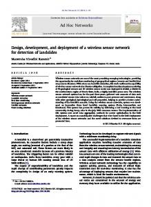
Fig. 1.
AVATAR Autonomous Helicopter
node, which is incorporated into the existing network. This approach to autonomous deployment of sensor networks will allow the on-demand instrumentation of remote environments that may be inaccessible by ground methods, and supporting applications to navigation, monitoring, and search and rescue. We have implemented the deployment algorithms on a hardware platform that integrates hardware and software from three labs: USC’s helicopter, Dartmouth’s sensor network, and CSIRO’s interface between a helicopter and a sensor network. The three groups conducted joint experiments which demonstrate, for a desired network topology, (1) autonomous sensor network deployment with a helicopter, (2) ground to ground and ground to air connectivity measurements for the resulting network and (3) uses the results to repair the network connectivity when the deployed topology does not match the desired topology. II. R ELATED W ORK Our work builds on important previous work in sensor networks and robotics, and bridges the two communities by integrating autonomous control of flying vehicles with multihop message routing in ad-hoc networks. Autonomous aerial vehicles have been an active area of research for several years. Autonomous model helicopters
have been used as testbeds to investigate problems ranging from control, navigation, path planning to object tracking and following. Flying robot control is a very challenging problem and our work here builds on successes with hovering for two autonomous helicopters [1], [2]. Several other teams are working on autonomous control of helicopters. A good overview of the various types of vehicles and the algorithms used for control of these vehicles can be found in [2] . Recent work has included Autonomous Landing [3], [4] Aggressive maneuvering of AFV’s [5] and pursuit-evasion games [6]. Research in sensor networks has been very active in the recent past. An excellent general introduction on sensor networks can be found in [7]. An overview of hardware and software requirements for sensor networks can be found in [8] who describe the Berkeley Mica Motes. Algorithmic work for positioning a sensor network where sensors have mobility and can self-propel includes even dispersal of sensors from a source point and redeployment for network rebuilding [9], [10]. Other important contributions include [11]–[15]. In our previous work on networked robots we used flying helicopters to localize a deployed sensor network [16], we computed and represented paths in sensor networks that could guide the motion of a mobile node such as a helicopter [16], [17], and we used sensor network mobility to cover a given area while maintaining connectivity [18]. III. D EPLOYMENT C ONTROL Our approach to deployment consists of three phases. In the first phase, an initial network deployment is executed. In the second phase, we measure the connection topology of the deployed network and compare that to the desired topology. If they match, the procedure is complete. Otherwise the measured connectivity graph is used to compute new deployment locations that will repair the desired topology. The last two phases can be run at any point in time to detect the potential failure of sensor nodes and ensure sustained connectivity. The same approach can also be used to increase the sensor density in an area. A. Deployment Algorithm Our goal is to develop control algorithms that allow a flying robot to deploy a sensor network with a specified communication topology. Given a specified network topology, and a deployment scale, we embed the topology in the plane and extract desired node locations from the resulting embedding. Network topology is represented as a graph whose edges correspond to sensors. Edges connect sensors who are within communication range of each other (with two-way communication between the nodes.) Embedding such a topology in the plane reduces to computing actual GPSs coordinates for the sensors to be deployed. The scale of the embedding is determined by the inter-node communication range. We then sort and convert the resulting points to waypoints in a way that optimizes the robot’s required trajectory for covering the points. We assume the robot can hover and deploy a node at
Fig. 2.
Deployment Mechanism on the Helicopter
each point and later in the paper explain the mechanism used to accomplish this. Algorithm 1 Algorithm for controlling an autonomous helicopter to deploy a sensor network. Input: desired network topology Initialization: Embed topology in the plane at the desired scale and extract waypoints. Sort waypoints into buckets by their x coordinate. for each x bucket do Sort waypoints by y. while more sensors in the deployment mechanism do go to next way-point hover deploy sensor
B. Connectivity Measurement Algorithm A Mote sensor that has been specially modified to add physical user interface controls (a potentiometer and switch) is used to control and configure the sensor side of the connectivity tests as shown in Algorithm 2. The controls are set for the number of ping iterations and whether the sensors should reply to pings or not and then a multi-hop message is broadcast to the sensors to start an experiment. A reset message can also be sent to reset the sensor to an initial state. Data collected during the experiment is later read from the sensors via a laptop basestation that sends a download command and reads the data via RF messages. C. Connectivity Repair Algorithm Our general repair algorithm has the following structure. The connectivity algorithm results in a connectivity graph. We can compare this graph against the desired topology embedding using graph isomorphism algorithms [19], [20]. If the two graphs are isomorphic we are done. If they are not
Algorithm 2 Algorithm for controlling the mote side of a connectivity experiment. Wait for experiment configuration/start message Initialization: Set configuration mode = air-to-ground, ground-to-ground, or ground-to-air. Set count = number of ping iterations. Send a multi-hop forwarding of start message to other motes. Thread 1 for i=1 to count do if mode = ground-to-ground OR mode = ground-to-air then broadcast a ping message. Sleep a random interval Thread 2 while Listen for messages do if message is a ping then if mode = air-to-ground OR mode = ground-to-ground then reply to ping. else if Message is a ping reply. then tabulate reply. Termination: broadcast counts of replies per mote ID in response to download message.
their difference can be computed using subgraph embeddings. This step results in a list of missing graph nodes and their coordinates, which can be represented as a set of waypoints. These are given as input to Algorithm 1. In our implementation we have used a simplified version of this procedure. We wish to deploy sensor networks whose connectivity graph is one connected component. Therefore the task of the connectivity repair algorithm is to determine the number of connected components in the deployed network. Algorithm 3 shows the protocol for determining the number of connected components. The sensors broadcast their ids and forward the ids they hear. Each sensor keeps the largest value it hears. The number of distinct values is the number of connected components in the graph. The helicopter can collect this information and determine how many components there are. If the network has at least two connected components we compute the separation region and determine how to cover it with waypoints in a way that connects the two components. In the simplest algorithm we compute the line segment between the two closest nodes in the disconnected components and determine waypoints along that line using the sensor communication range. A different approach is to compute the region of separation between the two connected components and randomly pick waypoints in that region.
Algorithm 3 Distributed algorithm for identifying the connected components in a sensor network. All the nodes in one connected component will have the same component value as a result of this protocol. for each node in the sensor network do component = id for each node in the sensor network do broadcast node id. while listen for newid broadcasts do if received id > component then component = newid broadcast newid Helicopter collects all component values Helicopter determines unique component values as the number of connected components.
IV. E XPERIMENTS We have implemented the algorithms for deployment and network connectivity using a sensor network with 50 nodes and an autonomous flying robot. Our experiments targetted the three main control tasks: (1) deployment; (2) connectivity measurements; and (3) repair. We executed each of these tasks in manual mode (where the helicopter was controled by a pilot) and in autonomous mode (where the helicopter operated fully autonomously once in the air.) In this section we describe our testbed and present some of the data collected from these different sets of experiments. A. The Helicopter Our experimental testbed, the AVATAR (Autonomous Vehicle for Aerial Tracking And Reconnaissance) [21] is a gaspowered radio-controlled model helicopter fitted with a PC104 stack augmented with sensors (Figure 1). A Novatel RT-2 DGPS system provides position data with a 2 cm CEP, Crossbow VGX 6-axis IMU unit provides rate information to the onboard computer where it is fused using a 16-state Kalman filter. The ground station is a laptop that is used to send highlevel control commands and differential GPS corrections to the helicopter. Communication with the ground station is carried via 2.4 GHz wireless Ethernet. Autonomous flight is achieved using a behavior-based control architecture [3]. B. The Sensor Network Our sensor network platform is the Berkeley Mica Mote [8]. The Mote hardware configuration includes a main processor board with a microcontroller that handles data processing tasks, A/D conversion of sensor output, state indication via LED’s, serial I/O, and control of a low-power radio transceiver. It consists of an Atmel ATMega128 microcontroller (with 4 MHz 8 bit CPU, 128KB flash program space, 4K RAM, 4K EEPROM), a 916 MHz RF transceiver (50Kbits/sec, 100ft range), a UART, an Atmel AT90LS2343 coprocessor, and a 4Mbit serial flash memory. The radio communication consists
of an RF Monolithics 916.50 MHz transceiver (TR1000), antenna, and some components to adjust the physical layer characteristics such as broadcast power and transmission rate. An auxiliary sensor board contains light, sound, and temperature sensors with space for adding other types of sensors. Sensor boards can be stacked for additional sensor functionality. A Mote runs for approximately one month on two AA batteries. The operating system support for the Motes is provided by TinyOS, an event-based operating system. Our testbed consists of 50 Mote sensors deployed in the form of a regular 7×7 grid, see Figure 3. An extra Mote sensor is fitted to the helicopter using a system developed by CSIRO, see Section IV-D.
Sensor Modality (Vision/GPS)
If position within threshold
Position and Orientation of Object
Deploy
Deployment Mechanism
Low Level Controller
Fig. 4.
Deployment architecture
controller, it tasks the helicopter to deploy an object or sensor at that location. This division of controllers ensures that the autonomous control of helicopter is completely decoupled from the task at hand. Hence if a new sensor (e.g. vision) was used for deployment instead of GPS, only the higher level controller needs to be changed. Fig. 3.
Helicopter Deploying Sensors in a 7 × 7 grid
C. The Deployment Mechanism The deployment mechanism consists of a radio controller(RC) servo which rotates a wire coil. The sensors to be deployed are attached to the loops on the coil at even intervals, and are dropped off the coil one at a time when it has rotated the specified number of rotations. A toggle switch is used to count the number of rotations. In this way we can accurately time and drop sensors at the given GPS location, see Figure 2. The architecture for deployment consists of a two stage controller (see Figure 4). The higher level controller depends on the sensor modality being used (either GPS or vision). For GPS based deployment, the controller obtains the current position of the helicopter from GPS and continually checks whether it is sufficiently close to a drop location, if it is then a deploy command is sent to the low-level controller. For vision based control a Kalman filter continually updates the estimate of the object and if the estimate is within the required error a deploy command is sent to the low-level controller. The primary function of the low-level controller is to keep the helicopter in hover and also to navigate the helicopter to the desired way-points. Once this controller receives a command for deployment from the higher level deployment
D. The Helicopter-Sensor Network Interface The helicopter carries one Mote to allow communications with the deployed sensor network. The Mote is plugged onto a programming and serial interface board which is serially connected to the helicopter’s linux computer. Several applications were run, depending on the experiment. The ping application sends a broadcast message with a unique id once per second and logs all replies along with the associated Mote identifier. This data allows us to measure air-ground connectivity, and results are presented in IV-G. The gps application receives GPS coordinates via a socket from the helicopter navigation software and broadcasts it. Simple algorithms in each Mote are able to use these position messages to refine an estimate of their location [16]. E. Experimental Procedure Our field experiments have been performed on a grass field on the USC campus. We marked a 7 × 7 grid on the ground with flags. We used an empirical method to determine the spacing of the grid. We established that on that ground, the Mote transmission range was 2.5 meters1 . We selected the grid 1 This communication range is much lower than the expected range for Motes. We believe the reduced range is due to the close proximity of the ground which absorbs a significant amount of RF energy, particularly when moist.
6
spacing at 2 meters so that we would guarantee communication between any neighbors in the field.
5 300 37
36 13 18 38
35
41
20 19
2
39
9
100
1 40
3 10
0
11
8
14
−100
12
4 number of responses
16 200
3
2 −200 0
200
Fig. 5.
400
600
800
1000
1200
Measured Position of the Sensors.
1
3
2.5
0
0
100
200
Occurrence
2
300 ping number
400
500
600
1.5
Fig. 7.
Number of responses to ping messages (by message).
1
0.5
0
70 0
0.5
Fig. 6.
1
1.5 2 2.5 Deployment error (m)
3
3.5
4
60
Histogram of deployment error.
F. Deployment using an Autonomous Helicopter The helicopter is given a waypoint file with the GPS location (x, y, z) coordinates where the sensors need to be deployed. It then flies to each of those points and drops the sensors. Figure 5 indicates the measured position of the sensors deployed with respect to the actual position to be deployed. Figure 6 shows a histogram of sensor deployment error distance which has a median value of 1.2 metres. In this particular set-of experiments the deployment was done manually. The Helicopter was being teleoperated by a pilot on the prescribed flight path. When the helicopter was within a radius of 1.5 meters from the deployment location a “drop” command was issued to deploy the motes. Completely autonomous deployment experiments were also performed, although we haven’t collected connectivity data for them yet. G. Air-to-ground connectivity The number of responses to each air-to-ground ping is shown in Figure 7. The maximum number of responses to any ping was 6 and the mean number was 2.1. In our experience the Mote radio is probabilistic with only a modest probability that a message is successfully transferred. It is very likely that more Motes received the ping and transmitted responses than the number of responses which were actually received. The number of responses by mote id is shown in Figure 8 where we can see that only 19 motes (39%) responded. This is a not a limitation of the motes, but a fact of the path
number of pings
50
40
30
20
10
0
0
10
Fig. 8.
20
30 mote id
40
50
Number of responses to ping messages (by mote).
flown during the experiment. The range over which these motes responded is shown in Figure 9 where we see that the maximum range was nearly 13 meters, but the median range was 9 meters. Note that the air-to-ground range is much greater than the 2.5 meter ground-to-ground range we measured, which is a typical asymmetry between ground-toground and air-to-ground radio transmissions. H. Ground to ground connectivity The sensor network as first deployed exhibited some disconnection in communications between sensors. This was measured by having each of the fourteen sensors broadcast ping messages and listen for replies from its neighbors. Figures 10
60
14
12
maximum distance (m)
10
8
Fig. 11.
Connectivity of the originally deployed sensors.
6
4
2
0
0
10
20
30 mote id
40
50
Fig. 9. Maximum range at which ping message was acknowledged (by mote).
12 14
16
13
10
20
3
18
1
19
9
35
2
60
Fig. 12.
Connectivity of the repaired network of deployed sensors.
1) now participating in the network. Sensor 1 was found to have been disconnected due to a hardware failure in its radio transceiver. Note that the connectivity of the outlying sensors (8, 14, 19, 20) has been improved even though the sensors that were deployed to improve connectivity were not near them. While intuitively this may not appear to make sense, there are a variety of factors that can account for it. In particular, increases in message traffic can alter packet collision characteristics which could improve connectivity in areas. For example, note that although the connectivity between 20 and 14 improved, the connectivity between 14 and 19 did not. This suggests that deployment patterns for network repair may need to take into account some characteristics of the radios used in the sensor network. E.g., VHF radios which can penetrate obstacles may require a different repair strategy than UHF radios which are line of sight.
8
I. Lessons Learned Fig. 10.
Connectivity of the originally deployed sensors.
Our experiments have given us several insights into mobile networks. •
and 11 show the resulting connectivity pattern as both a circular connection diagram and a diagram with the sensors in their actual locations. Each sensor is a vertex in the graphs and the lines show which sensor could communicate via a round trip path with its neighbors. The thickness of the lines correspond to the percentage of ping replies received, with thicker lines indicating better connectivity. Although connectivity is good between some of the motes, overall the graphs are sparsely linked indicating disconnection in the network. Based on this connectivity analysis another seven motes were deployed from the helicopter to repair the communication gaps. Figures 13 and 12 show the result of the round trip connectivity analysis on the repaired network. Connectivity has been greatly improved, with all sensors (except sensor
•
•
•
The communication range is highly dependent on relative antenna orientation, shielding (eg. helicopter between two Motes), and when close to the ground, on ground moisture. We found widely different ranges in Brisbane, LA, Dartmouth, and Pittsburgh. The communication links are asymmetric and congestion is a significant concern. In all our experiments two passes with the helicopter were required for deploying and subsequently repairing the network. With Good Control of the Helicopter a disconnected network can be repaired in one more pass. Note that this assumes that the Helicopter can carry the required number of sensors to repair the network and the topology for repair is known.
R EFERENCES
1
41
2
40
3
39
8
38
9
37
10
36
11
35
12
20
13 19
14 18
Fig. 13.
•
16
Connectivity of the repaired network of deployed sensors.
Deployment strategies are likely to need to be tailored to sensor radio characteristics such as range, obstacle penetrating capabilities, and antenna patterns. V. C ONCLUSION
We have described control algorithms and experimental results from sensor network deployment with an autonomous helicopter. By sprinkling sensor nodes using a flying robot, we can reach remote or dangerous environments such as rugged mountain slopes, burning forests, etc. We believe that this kind of autonomous approach will enable the instrumentation of remote sites with communication, sensing, and computation infrastructure, which in turn will support navigation and monitoring applications. From what we’ve learned in these experiments we plan to develop systems for automatic network repair. This will require the ground sensors and helicopter to cooperate to identify network disconnections and guide the helicopter to appropriate locations for autonomous sensor deployment. ACKNOWLEDGMENT Support for this work was provided through the Institute for Security Technology Studies, NSF awards EIA-9901589, IIS-9818299, IIS-9912193, EIA-0202789 and 0225446, ONR award N00014-01-1-0675 and DARPA Task Grant F-3060200-2-0585. This work is also supported in part by NASA under JPL/caltech contract 1231521, by DARPA under grants DABT63-99-1-0015 and 5-39509-A 9 (via UPenn) as part of the Mobile Autonomous Robot Software (MARS) program. Our thanks to our safety pilot Doug Wilson for keeping our computers from (literally) crashing.
[1] G. Buskey, J. Roberts, P. Corke, P. Ridley, and G. Wyeth, “Sensing and control for a small-size helicopter,” in Experimental Robotics, B. Siciliano and P. Dario, Eds. Springer-Verlag, 2003, vol. VIII, pp. 476–487. [2] S. Saripalli, J. M. Roberts, P. I. Corke, G. Buskey, and G. S. Sukhatme, “A tale of two helicopters,” in IEEE/RSJ International Conference on Intelligent Robots and Systems, Las Vegas, USA, Oct 2003, (To appear). [3] S. Saripalli, J. F. Montgomery, and G. S. Sukhatme, “Visually-guided landing of an unmanned aerial vehicle,” IEEE Transactions on Robotics and Automation, vol. 19, no. 3, pp. 371–381, June 2003. [4] O. Shakernia, Y. Ma, T. J. Koo, and S. S. Sastry, “Landing an unmanned air vehicle:vision based motion estimation and non-linear control,” in Asian Journal of Control, vol. 1, September 1999, pp. 128–145. [5] V. Gavrilets, I. Martinos, B. Mettler, and E. Feron, “Control logic for automated aerobatic flight of miniature helicopter,” in AIAA Guidance, Navigation and Control Conference, Monterey, CA, USA, Aug 2002. [6] R. Vidal, O. Shakernia, H. J. Kim, D. Shim, and S. Sastry, “Probabilistic pursuit-evasion games: Theory, implementation and experimental evaluation,” IEEE Transactions on Robotics and Automation, Oct 2002. [7] D. Estrin, R. Govindan, J. Heidemann, and S. Kumar, “Next century challenges: Scalable coordination in sensor networks,” in ACM MobiCom 99, Seattle, USA, August 1999. [8] J. Hill, R. Szewczyk, A. Woo, S. Hollar, D. Culler, and K. Pister, “System architecture directions for network sensors,” in ASPLOS, 2000. [9] M. Batalin and G. Sukhatme, “Spreading out: A local approach to multirobot coverage,” in Distributed Autonomous Robotic Systems 5, 2002, pp. 373–382. [10] A. Howard, M. Mataric, and G. Sukhatme, “Mobile sensor network deployment using potential fields: A distributed, scalable so lution to the area coverage problem,” in Distributed Autonomous Robotic Systems 5, 2002, pp. 299–308. [11] G. J. Pottie, “Wireless sensor networks,” in IEEE Information Theory Workshop, 1998, pp. 139–140. [12] J. Agre and L. Clare, “An integrated architeture for cooperative sensing networks,” Computer, pp. 106 – 108, May 2000. [13] P. Gupta and P. R. Kumar, “The capacity of wireless networks,” IEEE Transactions on Information Theory, vol. IT-46, no. 2, pp. 388–404, March 2000. [14] A. Scaglione and S. Servetto, “On the interdependence of routing and data compression in multi-hop sensor networks,” in ACM Mobicom, Atlanta, GA, 2002. [15] Y. Chen and T. C. Henderson, “S-NETS: Smart sensor networks,” in Seventh International Symposium on Experiemental Robotics, Hawaii, Dec. 2000. [16] P. Corke, R. Peterson, and D. Rus, “Networked robots: Flying robot navigation with a sensor network,” in ISRR, 2003. [17] Q. Li, M. DeRosa, and D. Rus, “Distributed algorithms for guiding navigation across sensor networks,” in MOBICOM, 2003. [18] M. Batalin and G. S. Sukhatme, “Coverage exploration and deployment by a mobile robot and communication network,” in 2nd International Workshop on Information Processing in Sensor Networks, Palo Alto Research Center, Palo Alto, California, USA, April 2003, pp. 376–391. [19] D. Corneil and C. Gotlieb, “An efficient algorithm for graph isomorphism,” Journal of the ACM, vol. 17, no. 1, pp. 51–64, March 1970. [20] J. E. Hopcraft and J. K. Wong, “Linear time algorithm for isomorphism of planar graphs,” in 6th Annual ACM Symposium on Theory of Computing, Seattle, Washington, 1974, pp. 172–184. [21] University of Southern California Autonomous Flying Vehicle Homepage, “http://www-robotics.usc.edu/˜avatar.”