The International Federation of Automatic Control. Seoul, Korea, July 6-11, 2008. 978-1-1234-7890-2/08/$20.00 © 2008 IFAC. 1952. 10.3182/20080706-5-KR- ...
Proceedings of the 17th World Congress The International Federation of Automatic Control Seoul, Korea, July 6-11, 2008
Avoidance of Poorly Observable Trajectories: A Predictive Control Perspective Christoph B¨ ohm ∗ Rolf Findeisen ∗∗ Frank Allg¨ ower ∗ ∗
Institute for Systems Theory and Automatic Control,University of Stuttgart, Germany {cboehm,allgower}@ist.uni-stuttgart.de ∗∗ Institute for Automation Engineering, Otto-von-Guericke-Universit¨ at Magdeburg, Germany {rolf.findeisen}@ovgu.de
Abstract: Nonlinear systems can be poorly or non-observable along specific state and output trajectories or in certain regions of the state space. Operating the system along such trajectories or in such regions can lead to poor state estimates being provided by an observer. Such trajectories should be avoided if used for state-feedback control or monitoring purposes. In this paper, we outline two possible approaches to avoid weakly observable trajectories in the frame of nonlinear predictive control. The first approach is based on the use of a term in the cost functional that penalizes weakly observable trajectories and thus leads to avoidance of weakly or non-observable regions of operation. In the second approach, the observer error dynamics are directly considered in the prediction. Large state estimation errors lead to a large penalization in the cost functional and are thus avoided. The approaches are exemplified by considering an example system. Keywords: Observability, Observer Performance, Nonlinear Systems, Predictive Control, Stability 1. INTRODUCTION Observability for linear time-invariant systems is well studied and understood and there exist several equivalent ways to define observability (Krener (2004, 1994); Zeitz and Xia (1997)). For nonlinear systems, however, the question of observability, and of the design of suitable state observers, is significantly more challenging, even in the nominal case. One of the main differences from linear systems is the fact that the observability of a nonlinear system in general depends on the input applied and on the region of operation/measured output trajectory. The observability of the state might, for example, be lost at points where the observability map is non-invertible for the given state, input, and output. If such points are not considered in the observer, they can lead to deteriorating observer performance (Vargas (2003)). Thus, if used in the context of state-feedback via the certainty equivalence principle, they can cause deterioration of the performance of the closed-loop or even instability. In this work, we consider the questions of the avoidance of loss of observability and of improved observer performance along trajectories in the frame of predictive control. As shown, predictive control is well suited for such problems, since the applied input trajectories are based on the repeated solution of an open-loop optimal control problem considering a (nonlinear) model of the system ⋆ The authors gratefully acknowledge funding by the German Research Foundation (AL 316/5-1)
978-1-1234-7890-2/08/$20.00 © 2008 IFAC
for prediction. Since the future behavior of the system is predicted, one can penalize trajectories that would lead to poor observability or observer performance. We are not immediately interested in designing a stabilizing outputfeedback control scheme. Rather, we are interested in the question of avoidance of trajectories that might deteriorate observer performance or lead to loss of observability. Specifically we consider two separate, but closely related, problems. Firstly, we are interested in if weakly observable trajectories can be actively avoided by a suitable choice of the input signal. For this purpose, we propose to incorporate in the cost functional a term that strongly penalizes non-observable/weakly observable trajectories. Secondly, we are interested if the observer-error performance can be directly considered in the predictive controller itself. To this end, we propose to augment the predictive system state by the observer error dynamics and to penalize trajectories that lead to large observer errors. The remainder of the paper is organized as follows. In Section 2 we state the considered system class and provide a motivation for the considered problems. Section 3 shortly reviews the basics of nonlinear model predictive control. Section 4 considers the question of avoidance of weakly observable/non-observable trajectories in predictive control, while Section 5 presents a predictive control approach that directly takes the observer error in the prediction into account. The outlined approaches are exemplified by considering an example system. Conclusions are provided in Section 6.
1952
10.3182/20080706-5-KR-1001.3406
17th IFAC World Congress (IFAC'08) Seoul, Korea, July 6-11, 2008
2. PROBLEM SETUP AND MOTIVATION We consider nonlinear systems of the form
n
x˙ = f (x, u), x(0) = x0 ,
(1a)
y = h(x, u),
(1b)
m
Mathematical Formulation: In NMPC the future behavior of the system is predicted. Therefore, we introduce predicted states and inputs, x ¯ and u ¯. The predicted states may differ from the real system states x. In this paper the cost function J, that is minimized over the prediction horizon Tp , is for reasons of simplicity defined as
p
with x ∈ R , u ∈ R and y ∈ R . Additionally, the system might be subject to state and input constraints of the form u(t) ∈ U ∀ t ≥ 0, x(t) ∈ X ∀ t ≥ 0.
� � J x¯(·), u¯(·) =
Here X ⊆ Rn is the state constraint set and U ⊂ Rm is the set of feasible inputs. For many purposes, such as state feedback control or monitoring the states of the system (1) must be recovered from the measurements. Even though that significant progress with respect to state estimation for nonlinear systems has been made in recent years, it is still a challenging and difficult task. One of the key differences from state estimation for linear systems is that observability for nonlinear systems generally depends on the inputs applied, outputs measured, and the system state itself. The system might be observable for certain regions in the state space, while observability might be lost in others. As an example, consider a system with a single output of the form y = x u. Clearly, if the controller chooses u = 0, the state cannot be reconstructed from the measurements (at least locally). In practical problems, sensors might saturate far away from their nominal point of operation, or they might deliver deteriorated measurements. Considering this problem, the question arises, if inputs and states that lead to a loss of observability, or weak observability, can be avoided. We outline in Section 4 a possible approach based on the ideas of predictive control. In contrary to the problem of loss of observability one might also ask, if it is possible to design trajectories such that a given observer will achieve good state estimates. This will be discussed in Section 5. Before we derive suitable methods to improve observer performance or avoid loss of observability, respectively, we first review in the following section the principle of nonlinear model predictive control. 3. NONLINEAR MODEL PREDICTIVE CONTROL Many research activities have focused on nonlinear model predictive control (NMPC) in recent years. Its ability to explicitly deal with nonlinear systems subject to state and input constraints gives the NMPC control method significant advantages when compared to many other control techniques. The basic idea of predictive control is as follows: by solving a finite horizon optimal control problem online based on current measurements of the system, an optimal control trajectory is obtained. The first part of this trajectory is applied to the system and the optimal control problem is solved again on the basis of new measurements at the next sampling instant. Several NMPC approaches exist to guarantee stability of the closed-loop system in case of state feedback NMPC, see Mayne et al. (2000), Fontes (2000), Findeisen (2004), and Camacho and Bordons (2007) for an overview.
tk +Tp
x ¯T Q¯ x + u¯T R¯ u dτ tk T
(4)
+ x¯ (tk + Tp )P x ¯(tk + Tp ),
(2) (3)
�
T
with 0 < Q = Q ∈ Rn×n , 0 < R = RT ∈ Rm×m and 0 < P = P T ∈ Rn×n . Hence, the open-loop optimal control problem that is solved repeatedly at the sampling instances tk is formulated as � � ¯(·), u ¯(·) , min J x
(5a)
u ¯ (·)
subject to
� � x¯˙ (τ ) = f x¯(τ ), u¯(τ ) , x¯(tk ) = x(tk ), � � x¯(τ ) ∈ X , u ¯(τ ) ∈ U, ∀τ ∈ tk , tk + Tp , x¯(tk + Tp ) ∈ Ex .
(5b) (5c) (5d)
Note that the predicted states x ¯ are forced to lie in the so called terminal region Ex at the end of the prediction horizon, which might be necessary to enforce stability. The solution of the optimization problem leads to the optimal input trajectory � � � � u ¯⋆ t; x(tk ) = arg min J x ¯(·), u¯(·) . u ¯ (·)
(6)
Here u ¯⋆ denotes the optimal input which minimizes the cost function J over the prediction horizon. The control input applied to system (1a) is updated at each sampling instant tk by the repeated solution of the open-loop optimal control problem (5), i.e. the applied control input is given by � � u(t) = u ¯⋆ (t; x(tk )), t ∈ tk , tk + δ ,
(7)
where δ is the sampling time between each optimization (assumed to be fixed). The following well known lemma guarantees stability in the sense of convergence of the closed-loop: Lemma 1. Assume that the stated assumptions on Q, R and P hold. Furthermore, assume that there exists a local control law u ˜ = k(x) ∈ U such that ∂xT P x f (x, u ˜) + xT Qx + u ˜T R˜ u < 0 ∀ x ∈ Ex . (8) ∂x Then the closed-loop is stable in the sense that x → 0 as t → ∞, if the open-loop optimal control problem is feasible at the time instant t0 . For reasons of simplicity the detailed assumptions and conditions for Lemma 1 are not discussed here (compare for example Findeisen (2004) and Fontes (2000)).
1953
17th IFAC World Congress (IFAC'08) Seoul, Korea, July 6-11, 2008
Remarks about output feedback: NMPC requires the repeated solution of an open-loop optimal control problem based on full knowledge of the system states. Thus, in most cases NMPC has to be combined with an observer that reconstructs the states of the system from the measurable outputs. Since for nonlinear systems no general valid separation principle exists (Teel and Praly (1994)), a combination of a state feedback controller with an observer does not necessarily lead to stability. By now several results with respect to output feedback NMPC exist (see e.g. Goulart and Kerrigan (2007); Mayne et al. (2006); Magni et al. (2004); Findeisen and Allg¨ ower (2004) and the references provided there). However, most of these approaches consider only either systems that are uniformly globally observable, or linear, or based on the assumption that the observer achieves sufficiently fast observer error convergence for all states and inputs encountered. Note that we do not intend to provide a solution to the output feedback NMPC problem here. We rather intend to take the observability properties of the system, or the observer dynamics in the NMPC controller, into account to avoid deteriorated state estimates along nominal trajectories. 4. AVOIDING WEAKLY OBSERVABLE TRAJECTORIES The loss of observability along optimal trajectories can lead to poor observer performance and therefore to severe problems in output feedback NMPC. This section provides an approach to overcome this problem. Problem Description: The solution of an open-loop optimal control problem in general does not guarantee system properties such as observability along the obtained optimal trajectories. Since predictive control implies the repeated solution of an open-loop optimal control problem, this implies that an NMPC controlled system may be steered to non-observable or poorly observable regions by the controller which should in general be avoided. The basic idea for a solution to this problem is to add a suitable penalization term to the objective functional (4) that penalizes weakly observable trajectories. In general, it is hard to find a suitable observability measure. For sake of simplicity, in the frame of this paper we limit our attention to local observability. For this we propose the use of the determinant of the local observability matrix, which is based on the observability map, as a measure of observability. One possible way to verify observability is the consideration of the observability map q(x, u) (see Vargas (2003) and the references provided there) for the system (1), which is is defined as
The determinant of the observability matrix det(O) can be used as a measure for observability of the considered system. If det(O) = 0 holds, the rank of O is clearly smaller than n and thus the system is not observable. Furthermore, small values of det(O) imply weak observability of the considered system since in this case the observability matrix is close to singular. In the frame of this paper, we consider observability along predicted trajectories x¯ and u ¯. Thus, the system is observable along the considered trajectory if the observability matrix has full rank along the complete trajectory. In the following an extension of the common state feedback NMPC scheme is presented which uses the observability matrix to avoid the fact that the system is steered to weakly respectively non-observable regions. Controller Modification: In general, if the solution of an open-loop optimal control problem guarantees observability along the obtained trajectories, this clearly also holds for state feedback NMPC trajectories based on this optimal control problem. One solution to guarantee observability along optimal trajectories, which presents itself, is to extend the open-loop optimal control problem (5) by a constraint on the observability matrix O (10). Basically, one can add the following constraint requiring that the determinant of the observability matrix is always larger than a minimum value Ωmin to the optimal control problem (5) � � |det O(¯ x, u ¯) | ≥ Ωmin . (11) The resulting optimal input u¯⋆ clearly assures observability of the obtained optimal trajectory. Furthermore, the design parameter Ωmin , if chosen large enough, even avoids steering the system to poorly observable regions. The main drawback of the inequality constraint (11) is that it is difficult, in general, to guarantee satisfaction of the constraint for all time points if the problem is solved numerically. As an alternative, a suitable penalization term in the cost function may be numerically easier to handle. One possible modification of (4), depending on the observability matrix O (10), might be � � J x ¯(·), u¯(·) = �
tk +Tp
x¯T Q¯ x+u ¯T R¯ u + ∆(¯ x, u ¯) dτ. (12)
tk
Here ∆(¯ x, u ¯) is given by α � �, |det O(¯ x, u¯) | where α is an positive design parameter. ∆(¯ x, u ¯) =
(m−1)
q(x, u) = [y, y, ˙ ··· ,y ]. (9) Basically, the considered system is locally observable if the nonlinear observability matrix O, defined as the Jacobian of the observability map q, ∂q(x, u) , (10) ∂x has full rank n for all x ∈ X and all u ∈ U. It is locally observable at some point xs if O(xs , u) has full rank at this point xs for all u ∈ U. In the following the expression observability is used to mean local observability. O(x, u) =
Remark 1. Note that for simplicity of presentation we assume that the observability map does not depend on the input derivatives.
(13)
The consideration of the determinant of the observability matrix O(¯ x, u ¯) in this form will lead to an�increase� of the modification term ∆(¯ x, u ¯) to infinity if |det O(¯ x, u ¯) | → 0. This implies that the solution to the open-loop optimal control problem, with the modified cost function (12), will avoid poorly or non-observable trajectories since those are weighted heavily in the cost function. Therefore, the (state feedback) NMPC controlled system will also not enter poorly observable regions (if no disturbances are present).
1954
17th IFAC World Congress (IFAC'08) Seoul, Korea, July 6-11, 2008
α � � � �, (14) max |det O(¯ x, u ¯) |, Θ where the design parameter Θ is used to obtain an upper bound for ∆(¯ x, u ¯). This implies that non-observable or very poorly observable trajectories can be reached by the system, however, at the price of a very strong penalization in the cost function (if Θ is chosen to be sufficiently small). Thus, the system can pass non-observable regions if the control objective demands for it, but it will only stay there for as short a time as possible.
The required design parameters are chosen as (19) R = 0.1, q1 = q2 = q3 = 1, α = 2, θ = 0.05, with Q being a unity matrix. Figure 1 shows simulation results for x1 and the modified cost function value for the nominal NMPC controller without considering the penalization term and the NMPC controller with the penalization term starting at x10 = 0.6 and x20 = −2 x30 = −0.5. As is clearly visible, the penalization approach avoids having the system pass through x1 = −1. As a summary, the modified approach avoids steering the system to poorly observable regions if the control objective allows for the avoidance of such regions. 1 0.5 0 x1
Both approaches, introduction of a further constraint and extension of the cost function, respectively, have one main drawback. The control objective could be such that it is impossible to avoid steering the system through a singularity of O(¯ x, u ¯). To illustrate this, consider the following simple example. The control objective is to steer a system with a�singularity �of the observability matrix at x1 = 1, i.e. det O(x1 = 1) = 0, from x1 (0) = 2 to the origin. This control objective cannot be satisfied without crossing the singularity � �x1 = 1. In such cases the modified constraint |det O(¯ x, u ¯) | ≥ Ωmin (11) prevents the system from crossing the singularity of the observability matrix. In the second approach, ∆(¯ x, u ¯) would act as a barrier function and the solution of the optimal control problem would lead to trajectories with x1 > 1 since the value of the cost function (12) rises to infinity otherwise. To avoid this, equation (13) can be extended by
−0.5
∆(¯ x, u ¯) =
−1 −1.5
0
1
2
3 time
4
5
6
0
1
2
3 time
4
5
6
1 0.8
|det(O)|
0.6 0.4 0.2 0
All of the approaches presented above guarantee observability of the considered system along the obtained optimal trajectories. Remark 2. (Stability) We do not outline conditions for stability. It is clear that the addition of the inequality constraint (11) does not change the stability properties, e.g. if the problem is initially feasible stability is guaranteed. Guaranteeing stability in the case of the modified cost function (12) or (14) is more involved. One basically has to verify that the conditions of Lemma 1 still hold or that the penalization factor is chosen suitably. Example:
Consider the nonlinear system x˙ 1 = x2 x˙ 2 = x1 + x2 + (1 − x21 )x3 + u x˙ 3 = −x1 + x3
y = x1 . The corresponding observability map is x1 x2 q(x, u) = 2
x1 +x2 +(1−x1 )x3 +u
(16)
and the observability matrix becomes � 1 0 0 0 1 0 (17) O(x) = 1−2x1 x3 1 1−x21 � � with the determinant det O(x) = 1 − x21 . Obviously, the system is not observable for x1 = 1 and x1 = −1. For the given system, the modification term (14) becomes ∆(¯ x, u ¯) =
α � �. max |1 − x21 |, Θ
(18)
−0.2 −0.4
Fig. 1. Solid line: classical NMPC formulation. Dashed line: NMPC formulation with penalization of “weak observability”. 5. GUARANTEEING GOOD OBSERVER PERFORMANCE Even if an NMPC controlled system is observable along all possible trajectories, few conclusions can be drawn concerning the observer, and overall output feedback performance. For example, it still might be possible that the observer error converges to zero very slowly although the system is observable. In the following, we outline a minmax based approach that guarantees the achievement of a predefined observer error dynamics behavior along the predicted trajectories thus guaranteeing stability of the closed-loop system. The observer is assumed to be given and of the form x ˆ˙ = fˆ(ˆ x, y, u), xˆ(0) = x ˆ0 ,
(20)
n
where x ˆ∈R . Modified NMPC Scheme: The basic idea of the approach is that not only the behavior of the considered system is predicted into the future but also the observer behavior. For this, the worst-case error dynamics are determined via maximization of the estimation error in the prediction horizon over the set of all possible initial estimation errors at the time instant tk . Furthermore, a barrier function is
1955
17th IFAC World Congress (IFAC'08) Seoul, Korea, July 6-11, 2008
employed which only allows such inputs which guarantee that the observer satisfies desired reference error dynamics, even with the worst-case initial estimation error. The classical part of the NMPC scheme with the prediction of the system states remains. Classical output feedback NMPC schemes assume that the certainty equivalence principle holds, i.e. x(tk ) = x ˆ(tk ), where x represents the system state and x ˆ the observer state. As a consequence of this, these approaches use the observer state x ˆ at the corresponding time instant tk as initial condition for the predicted system states x ¯ (i.e. x ¯(tk ) = x ˆ(tk )), in order to predict the system behavior. However, often system and observer states differ. Therefore, in addition to the classical prediction of x ¯, the approach considers that we do not know the exact state of the system at the beginning of the prediction horizon. It is assumed that at the time instant tk the observer has an estimation error e¯0 ∈ E0 , i.e. in order to predict the observer error a new prediction state x ¯d is introduced with initial condition x¯d (tk ) = x ˆ(tk ) − e¯0 . The additional prediction state x ¯d is introduced to distinguish from the classical variable x ¯, which is predicted in parallel. The new state x ¯d leads to a predicted output y¯d = h(¯ xd , u¯) which enters the observer equation and thus leads to a predicted ˆ observer state x ¯d . The prediction states of the system and the observer define the predicted error e¯ = xˆ ¯d − x ¯d .
The basic idea is to maximize the error (21), i.e. to find the worst-case initial condition the real system may have (at a certain time instant tk , state estimation x ˆ(tk ) and for a given input function u ¯), such that the observer converges slowest to the predicted system state xd . This worstcase initial estimation error is denoted as e⋆0 ∈ E0 . The corresponding maximization problem 1 , which depends on a given input function u ¯ and on the observer state at the time instant tk , xˆ(tk ), is defined by
e0 ∈E0
�
For simplicity, we only consider linear reference dynamics 1 with a fixed convergence rate |λ| , i.e. er = e⋆0 eλ(τ −tk ) , where λ represents the eigenvalue of the chosen linear error dynamics. In the cost functional the worst-case error dynamics e¯⋆ are penalized heavily if it converges slower to zero than the reference error er and penalized weakly if the opposite holds. Thus, the optimal input u¯⋆ is such that the observer error satisfies the requirements of the reference error er even for the worst-case estimation error e⋆0 at the time instant tk . Furthermore, since the prediction of the estimation error occurs in parallel to the classical prediction of x¯, u ¯⋆ also takes the system performance requirements into account. The modified cost function (4) corresponding to the description above is formulated as � � J x ¯(·), e¯⋆ (·), u¯(·) =
�
tk +Tp
x ¯T Q¯ x+u ¯T R¯ u + Φ dτ tk
+ x¯ (tk + Tp )P x ¯(tk + Tp ),
with the additional observer error penalizing term Φ=
e¯⋆T e¯⋆ eTr er
,
� � min J x ¯(·), e¯⋆ (·), u ¯(·) , u ¯ (·)
subject to
ˆ(tk ), x ¯˙ = f (¯ x, u¯), x ¯(tk ) = x ⋆ ⋆ ⋆ ˙x ¯d = f (¯ xd , u ¯), x ¯d (tk ) = xˆ(tk ) − e⋆0
e¯T e¯ dτ ,
y¯d⋆ = h(¯ x⋆d , u ¯), ⋆ ⋆ ˙x ˆ ˆ¯⋆d (tk ) = x ˆ¯d = f (ˆ xd , y¯d⋆ , u ¯), x ˆ(tk ),
tk
xd , u ¯), x¯d (tk ) = x ˆ(tk ) − e0 , x¯˙ d = f (¯
x ¯ ∈ X, u ¯ ∈ U,
xd , u ¯), y¯d = h(¯ ˆ ˆ xˆ ¯˙ d = fˆ(x ¯d , y¯d , u¯), x ¯d (tk ) = x ˆ(tk ).
x ¯(tk + Tp ) ∈ Ex , e¯⋆ (tk + Tp ) ∈ Ee .
Together with the given input function u¯, the solution of the maximization problem,
The solution of the min-max-optimization problem leads to the optimal input trajectory � � � � u ¯⋆ t; x ˆ(tk ) = arg min J x¯(·), e¯⋆ (·), u¯(·) . u ¯(·)
e0 ∈E0
(25)
In summary, we obtain the following open-loop optimal control problem
subject to
�
tk +Tp
e¯T e¯ dτ ,
(23)
tk
leads to the related worst-case trajectories of the predicted ˆ¯⋆d system x ¯⋆d (with the output y¯d⋆ ), the predicted observer x ⋆ ⋆ ˆ¯d − and the predicted worst-case estimation error e¯ = x x ¯⋆d . The initial conditions for the prediction are x¯⋆d (tk ) = x ˆ(tk ) − e⋆0 and xˆ ¯⋆d (tk ) = x ˆ(tk ). 1
�β
where β ∈ N represents a further design parameter.
tk +Tp
e⋆0 = arg max
(24)
T
(21)
With respect to the initial estimation error e¯0 we only assume that e¯0 ∈ E0 holds.
max
Additionally, we introduce reference observer error dynamics er that should be achieved. Basically, these can be chosen arbitrarily and can be seen as a design parameter for the output feedback NMPC scheme.
Assuming for simplicity of presentation that the maximum exists and is attained
(27)
The terminal region of the presented NMPC scheme consists of the classical terminal region Ex and the terminal region Ee for the worst-case estimation e¯⋆ (tk + Tp ) defined as � � � � T n� e e (28) Ee = e, er ∈ R � T < 1 . � er er
The tuning parameter β allows one to use the modifying term (25) as a barrier function. If β is chosen large
1956
17th IFAC World Congress (IFAC'08) Seoul, Korea, July 6-11, 2008
enough, the additional cost function term (25) goes to zero if e¯⋆T e¯⋆ < eTr er , and to infinity if the opposite holds. This implies that if β is large enough the barrier function (25) restricts the set of admissible input functions u(·), since for all input functions u(·) violating the condition e¯⋆T e¯⋆ < eTr er , the cost function takes an infinitely large value. Furthermore, among all remaining admissible input functions the desired error dynamics is satisfied and thus (25) goes to zero. Hence, only the terms based on the classical prediction x ¯ influence the cost function. Therefore, for all input functions u(·) satisfying the desired error dynamics the performance of the controller is the same as in a classical output feedback NMPC scheme. Remark 3. (Stability) As a consequence of the introduction of a terminal region for the worst-case estimation error, namely Ee , the overall terminal region of the NMPC scheme presented above consists of Ex and Ee . The following lemma guarantees stability of the closed-loop system: Lemma 2. If the required assumptions and conditions on X , U, Ex , Q, R, P , f and on the feasibility of the optimal control problem at the time instant t0 hold, then the closed-loop is stable in the sense that x → 0 as t → ∞, if there exists a local control law u ˜ = k(x) with k(0) = 0 such that the following inequality ∂xT P x f (x, u˜) + xT Qx + u ˜T R˜ u+ ∂x
eT e eTr er
�β
< 0, (29)
is satisfied for all x ∈ Ex and all e, er ∈ Ee with u ˜ = k(x) ∈ U. We only outline the idea of the proof here: Since in the terminal region Ee the following inequality
� eT e < 1, (30) eTr er holds, it is trivial to show that there exists β large enough T β such that in (29) the modified term eeT eer vanishes. In r this case (8) is a suitable approximation of (29). Thus, if Lemma 1 holds, Lemma 2 also holds. Basically, the modified NMPC scheme has to satisfy exactly the same stability conditions as a classical NMPC controller (for sufficiently large β). The outlined scheme guarantees stability of the closed loop consisting of the observer and the controller. 6. CONCLUSIONS Nonlinear systems can be poorly or non-observable along specific state and output trajectories or in certain regions of the state space. Operating the system along such trajectories or in such regions can lead to poor state estimates provided by an observer and should be avoided
if being used for state-feedback control or monitoring purposes. In this paper we have outlined two possible approaches to avoid weakly observable trajectories in the frame of nonlinear predictive control. The first approach is based on the use of a term in the cost functional that penalizes weakly observable trajectories and thus leads to avoidance of weakly or non-observable regions of operation. In the second approach the observer error dynamics are directly considered in the prediction. Large state estimation errors lead to a large penalization in the objective function and are thus avoided. As shown, both approaches guarantee stability under certain conditions. REFERENCES E. F. Camacho and C. Bordons. Nonlinear model predictive control: An introductory review. In R. Findeisen, F. Allg¨ ower, and L.T. Biegler, editors, Assessment and Future Directions of Nonlinear Predictive Control, pages 1–16. Springer-Verlag, 2007. R. Findeisen. Nonlinear Model Predictive Control: A Sampled-Data Feedback Perspective. PhD thesis, University of Stuttgart, 2004. R. Findeisen and F. Allg¨ ower. Min-max output feedback predictive control with guaranteed stability. In Mathematical Theory of Networks and Systems, 2004. F. A. Fontes. A general framework to design stabilizing nonlinear model predictive controllers. System and Control Letters, 42(2):127–142, 2000. P. Goulart and E. Kerrigan. Output feedback receding horizon control of constrained systems. International Journal of Control, 80:8–20, 2007. A. J. Krener. State recovery by observers. To appear in Encyclopedia for Life Support Systems article contribution 6.43.21.15, 2004. A.J. Krener. Nonlinear stabilizability and detectability. In U. Helmke, R. Mennicken, and J. Saurer, editors, Systems and Networks: Mathematical Theory and Applications, pages 231–250, 1994. L. Magni, G. De Nicolao, and R. Scattolini. State and output feedback nonlinear model predictive control: An overview. International Journal of Robust and Nonlinear Control, 14:1379–1391, 2004. D. Q. Mayne, J.B. Rawlings, C.V. Rao, and P.O.M. Scokaert. Constrained model predictive control: Stability and optimality. Automatica, 36:789–814, 2000. D. Q. Mayne, S. Rakovic, R. Findeisen, and F. Allgwer. Robust output feedback model predictive control of constrained linear systems. Automatica, 42:1217–1222, 2006. A. Teel and L. Praly. Global stabilizability and observability imply semi-global stabilizability by output feedback. Syst. Contr. Lett., 22(4):313–325, 1994. A. Vargas. Observer design for nonlinear systems with reduced observability properties. Fortschr.-Ber. VDI Reihe 8 Nr. 999, VDI Verlag, D¨ usseldorf, 2003. M. Zeitz and X. Xia. On nonlinear continuouse observers. Int. J. Contr., 66(6):943–954, 1997.
1957