Sharp and feature edges which should be preserved can be checked during preprocessing. â¢. Intersections and inversions of tetrahedra inside and out- side of.
Eidgenossische ¨ Technische Hochschule Zurich ¨
Technical Report No. 287, January 1998
Institute of Scientific Computing
Ecole polytechnique federale ´ ´ de Zurich Politecnico federale di Zurigo Swiss Federal Institute of Technology Zurich
Computer Graphics Research Group
Avoiding Errors In Progressive Tetrahedralizations Oliver. G. Staadt, Markus. H. Gross Computer Graphics Research Group Institute of Scientific Computing Computer Science Department ETH Zürich, Switzerland E-mail: {staadt, markus.gross}@inf.ethz.ch WWW: http://www.inf.ethz.ch/department/IS/cg
Avoiding Errors In Progressive Tetrahedralizations Oliver G. Staadt, Markus H. Gross ETH Zurich
ABSTRACT
In this paper we elaborate on some pitfalls and fallacies people might get caught in when trying to implement the method of edge collapsing for tetrahedral meshes. Specifically, we address the issue of defining appropriate cost functions. Unlike the elegant geometric approach presented in [3], we must account for volume and application specific properties, such as volume preservation, gradient estimation of the underlying data or aspect ratio of the simplex. In addition, we devised a sequence of tests to guarantee a robust and consistent progressive tetrahedralization. Some results obtained on CFD data sets illustrate the performance of the PT1.
This paper describes some fundamental issues for robust implementations of progressively refined tetrahedralizations generated through sequences of edge collapses. We address the definition of appropriate cost functions and explain on various tests which are necessary to preserve the consistency of the mesh when collapsing edges. Although being considered a special case of progressive simplicial complexes [4], the results of our method are of high practical importance and can be used in many different applications, such as finite element meshing, scattered data interpolation or rendering of irregular volume data. CR Categories: I.3.5 [Computer Graphics]: Computational Geometry and Object Modeling – surfaces and object representations. Keywords: mesh simplification, multiresolution, FEM meshing.
2 PROGRESSIVE TETRAHEDRALIZATIONS For reasons of readability, we recapitulate some basic definitions for progressive meshes and adapt them to progressive tetrahedralizations (PT). General introductions are provided in [3] or [4].
1 INTRODUCTION
Background In PT representations, a tetrahedral mesh with scalar attributes s i assigned to each vertex v i is defined as
Progressive meshes [3] and its generalizations to higher dimensions [4] have proofed to be an extremely powerful notion for the efficient representation of triangulated geometric objects at different levels of detail. Although a general formulation for arbitrary triangulations has already been given in [4], the special case of progressive tetrahedralizations (PT) is of enormous practical importance, since it can be used as a sophisticated representation for a large variety of computations. Finite Element discretizations, from where our contribution was motivated, are one example. Here, sophisticated computational methods try to find an optimal balance between refinements of the mesh and of the polynomial degree of the basis functions. Other important applications of progressive tetrahedralizations comprise interpolation and rendering of scattered volume data, where successively refinable methods would definitely improve the performance of existing approaches. A general overview of various mesh simplification methods, including those based on edge collapses, can be found in [2]. However, regardless of the brilliance and simplicity of the idea of edge collapsing, a brute force implementation of the method may rapidly destroy the consistency of the mesh. Various artifacts can be introduced, such as flipped, intersected and degenerated tetrahedra, which in turn may kill any Finite Element computation. An example is given in Fig. 1. Here two boundary tetrahedra intersect due to an edge collapse in a locally concave mesh region.
( M 0, vsplit 0, vsplit 1, …, vsplit n – 2, vsplit n – 1 )
where M 0 is some coarse base mesh and vsplit i are vertex split operations to reconstruct the original mesh M = M n from M 0 : M
0
vsplit 0
M
1
vsplit 1
…
vsplit n – 1
n M .
(2)
M0
Conversely, is derived from M through a series of edge collapse operations ecol i which are inverse to vsplit i : M
n
ecol n – 1
M
n–1
ecol n – 2
…
ecol 0
0
M .
(3)
Each ecol i replaces an edge e i with vertices v a and v b by a new vertex v a . As opposed to some other methods we preserve the topological type of the mesh, that is, all instances of M are homeomorphic. Specifically, we prohibit degenerations of tetrahedra into lower dimensional simplices. The set of tetrahedra sharing e i will be called { icells i } . Thus, an edge split adds the tetrahedra in { icells i } to the list of active elements. Conversely, the set of nonvanishing tetrahedra affected by the associated edge collapse is called { ncells i } . Fig. 2 depicts an edge collapse operation in a tetrahedral mesh. All tetrahedra sharing e i vanish, whereas all tetrahedra sharing only one of the vertices of the edge change in shape. In order to compute a sequence of robust, non-degenerate and consistent meshes, the following aspects have to be considered: • Cost functions which determine the order of ecol operations depending on desired mesh optimization criteria. • Sharp and feature edges which should be preserved can be checked during preprocessing. • Intersections and inversions of tetrahedra inside and outside of { { icells i } ∪ { ncells i } } , such as the one in Fig. 1, have to be processed at run time. The remainder of this paper elaborates on the details of these issues.
collapsing edge
a)
(1)
Cost Functions Various elegant algorithms [1][3] based on
b)
the ecol/vsplit paradigm used cost functions optimized for triangular surfaces, often accounting for distance measures, triangle shape
Figure 1: Intersection of two tetrahedra: a) The edges of two non-adjacent tetrahedra bounding the volume intersect while collapsing an edge in a locally concave mesh region. b) Close-up of the intersection.
1 The
method is currently implemented as a set of AVS/Express modules and will be made available shortly.
1
v4
vb
Note that the initial mesh M n will usually be generated from some triangulation scheme. Depending on the application context and the desired mesh features it can be advantageous to include some ∆E edgelen(e i) = w edgelen ⋅ v a – v b into the cost function thereby enforcing short edges to be collapsed earlier. This term, however, is omitted in subsequent examples.
v4
v3 v3 v1
v2
Static Tests Unfortunately, brute force selection of edges
v2 va
v1 va
v5
according to the cost function from above can introduce mesh inconsistencies, like degeneration, folding, intersection, or loss of individual features. In order to avoid these types of artifacts, some static tests can be carried out prior to building the edge heap. Before we introduce the test criteria we have to define some properties of edges and vertices: • sharp edge: an edge e i is called sharp if it lies on the boundary of the mesh. • sharp vertex: a vertex v i is called sharp if at least one edge incident to v i is sharp. • sharp face: a triangular cell face f i is called sharp if all its edges are sharp. • sharp cell: a tetrahedral cell T i is sharp if at least one of its faces is sharp. Sharp edges can be detected efficiently by analyzing all vertices v j ∈ { icells i } assuming appropriate data structures to represent the mesh. In a preprocessing step we label all sharp vertices and edges, respectively. Table 1 lists the 5 different cases for combinations of sharp edges and vertices. Only cases 1 and 5 pass the consistency test.
{ ncells i } { icells i }
v5
a)
b)
Figure 2: Edge collapse in a tetrahedral mesh: a) Mesh before collapsing edge ( v a, v b ) . b) Configuration after collapse with resulting vertex v a . (Tetrahedra are shrinked to emphasize the underlying 3-dimensional structure.)
and others. In tetrahedral meshes, however, we have to redefine the terms of the cost function considering other features, like volume preservation or gradients. Although many different measures are conveivable to control the simplification process, the following ones yield a good balance between required degrees of freedom and the pain of parameter optimization. Thus, in our setting, for each edge e i = ( v a, v b ) , the associi i+1 ated edge collapse operation ecol i(a, b): M ← M is assigned the following cost: ∆E(e i) = ∆E grad(e i) + ∆E volume(e i) + ∆E equi(e i) .
(4)
Table 1: The 5 possible cases for combinations of sharp edges and sharp vertices. The examples refer to Fig. 3.
The first term ∆E grad is defined as ∆E grad(e i) = w grad ⋅ s a – s b
CASE e 1 2 3 4 5 sharp
(5)
and forms a simplified measure for the difference of underlying scalar volume function along the edge e i . Hence, edges with considerably differing scalar attributes are assigned high costs. When collapsing edges and removing tetrahedra from the mesh, the overall volume tends to decrease, that is the mesh shrinks down. Therefore, we introduce a second term ∆E vol penalizing volume changes: ∆E vol(e i) = w vol ⋅ +
∑
T j ∈ { icells j }
∑
T j ∈ { ncells i }
( vol(T j) – vol(T j) )
. (6)
v0
T j denote all tetrahedra in the set of neighborhood cells { ncells i } of e i and introduced cells { icells i } , respectively. vol(T j) stands for the volume of T j and T j is the tetrahedron after the collapse. Note that only simplices in { icells i } ∪ { ncells i } can contribute to volume changes. Especially in FEM applications, it is often required that tetrahedra sustain equilateral shape. ∆E equi can be employed in order to balance the edge length of tetrahedra:
∑
{ a, b } ∈ T j
( l a, b – m j )
∑
∑
T j ∈ ncells i { a, b } ∈ T j 2
2
( l a, b – m j ) –
vb
PERMISSIBLE
sharp sharp sharp
yes optionala optionala nob yesc
sharp sharp sharp
EXAMPLE
a: cases 2 and 3 induce “dents” on the boundary surface which may not be desired (similar to ∆E vol ). b: case 4 introduces degenerated cells, since v 9 is not deleted. c: a sharp edge always implies that it’s vertices are sharp. Simplifications of the boundary surfaces are allowed.
vol(T j)
∆E equi(e i) = w equi ⋅
va
v1
v 13
v 12
v 14
v2
v 11
v 15
v 16
v4
v5
v3
v 10
v9
v 17
v8
v7 v6
sharp vertex regular vertex
sharp edge regular edge
Figure 3: Naming conventions used for static consistency tests. For simplicity, the examples are depicted in 2D.
(7)
Dynamic Tests Unfortunately, not all inconsistencies can be fixed with the static tests from above. Some severe problems arise dynamically while performing individual ecol operations and further tests are required on the fly. Circumvention of folding or self-intersection of tetrahedra can easily be implemented by analyzing the volume of all T i ∈ { ncells i } before and after the collapse. Recall that the volume of a tetrahedron is defined by the parallelepipedial product of
with edge length l a, b = v a – v b and average edge length mj = 1 ⁄ T j ⋅ ∑ l . { a, b } ∈ T j a, b Each term can be weighted individually by a coefficient w to allow adoption to specific data sets and applications. 2
sharp
its 3 edges e i, e j and e k : 1 1 --- [ e i, e j, e k ] = --- 〈 e i × e j, e k〉 . 6 6
} with their non-visited neighboring ited tetrahedra in { T i sharp, m }are shown sharp cells and thereby traverse the mesh. The{ T i in Fig. 4c for different iteration steps. The following pseudo code summarizes the principle steps of the intersection test:
(8)
If the volume of one of the neighboring tetrahedra becomes negative, tetrahedral folding occurs. In this case the edge fails the consistency test. This test also avoids degenerate cells by setting a lower volume threshold to be retained after the collapse. We start from the following observation: edge collapses can cause global intersections of tetrahedra, a simple example of which is shown in Fig. 1. This requires additional testing. If the set { { icells i } ∪ { ncells i } } contains no sharp edge, it’s boundary forms a convex polytope entirely wrapping the edge. A collapse of the edge, however, does not affect the boundary of the polytope, whose disjoint triangulation is given by the tetrahedra T j ∈ { ncells i } . Thus, intersections can only occur with sharp cells and we can restrict the intersection tests to the mesh boundary. Fig. 4a depicts the top view of a tetrahedral mesh where T j is a sharp cell that is close to, but not intersecting the boundary of the mesh. Let e i be the edge to be collapsed next and let vertex v b be closer to the viewpoint than v a . The situation after the collapse where T j is intersecting two faces of { ncells i } is depicted in Fig. 4b.
intersection_test { // Tsharp[i,m]: sharp cells T i at iteration m // f[k]: sharp faces in ncells i // calculate_intersections: triangle-triangle // intersection test // M: maximum iteration level m = 0; while (Tsharp[i,m] not empty && m < M){ forall f[i] in Tsharp[i,m] forall f[k] calculate_intersections(f[i], f[k]); update Tsharp[i,m]; m++; } }
Note that the test asymptotically traverses all sharp faces of the mesh and consumes time proportional O(F ⋅ B) , where F stands for the number of elements in { f k } and B for the overall number of sharp faces in the data set. As we will demonstrate in Section 3, one can restrict the iteration to an upper bound in practice.
face intersection
ncells i
Edge Collapse After calculating the cost of each edge and determining the static conditions of the corresponding edge collapse operation, we build a heap with all remaining edges sorted according to their associated costs. In order to carry out the edge collapse ecol i , we pop the topmost edge from the heap, check for intersections, construct a vsplit i record for reconstruction, and update all edges on the heap which are in { ncells i } . This process is repeated until the heap is empty or the desired number of collapses has been reached. Although we implemented various schemes for the optimal positioning of v a , such as stochastic optimization, we found that the halfway between v a and v b is a good choice.
Tj va
e va
vb icells i
a)
b) ncells i sharp, 1
{T i va
}
sharp, 2 {T i } sharp, 3 {T i } sharp, 4 {T i }
3 RESULTS For the following investigations, an irregular mesh of a turbine blade was selected. The original data set consists of 576,576 tetrahedra with scalar node data representing pressure between the blades. Fig. 5 shows results with various levels of reconstruction, different settings of the cost functions, and extracted isosurfaces, both for the original mesh and for a selected subset with only one blade. Table 2 lists the performance statistics and parameter setn tings used to generate the example meshes. M denotes the origii nal number of tetrahedra and M is the number of tetrahedra of the reconstructed mesh. ∆E grad , ∆E vol , and ∆E equi indicate the individual cost function terms used for the example. Time shows the computation time for a full mesh collapse, i the number of vsplits, and Hits the number of dynamically deleted intersections ( m = 2 ). The performance of our algorithms was measured on an Indigo2 R10000@195MHz. The reconstruction time for the examples was between 0.1s and 0.8s, depending on the number of splits. Fig. 5a shows isosurfaces of the blades, extracted from
c)
Figure 4: Tetrahedron T j intersects two faces of { f k } after collapsing edge e i into vertex v a . a) before collapse. b) after colsharp, m } for iteration steps 1– lapse. c) Traversal of the mesh { T i 4.
In essence, we have to perform triangle–triangle intersection tests [5] in case of sharp edges or vertices which can be carried out as follows: First, we define the set of triangles { f k } containing all sharp faces of tetrahedra T j ∈ { ncells i } . These are the faces which can change after ecol i since they all share the new vertex v a . Thus they are our prime candidates for intersection with other sharp faces. In order to avoid testing these faces against all other sharp tetrahedra, we propose the following iterative method: The algorithm sharp } containing the subset of all sharp starts from an initial set { T i tetrahedra in the direct neighborhood of ncells i . sharp } and test for intersection We take the first element of { T i with all faces in f k . If the test fails and no intersection occurs, we label the tetrahedron as visited and proceed to the next element of sharp {T i } . Otherwise we can abort the test and reverse the current ecol i operation. The restriction to the sharp faces of each tetrahedron simplifies the intersection test, since many cell have only one sharp face (see Fig. 4). After probing all cells, we replace all vis-
15000
M at isovalue 5.0. A slice through the mesh is displayed in order to depict the irregularity of the mesh reconstruction. Note especially the high quality of the isosurfaces which confirms the effectiveness of ∆E grad . A subset of the mesh with one blade is shown in Fig. 5b-c for two different resolutions. In order to balance the individual terms of ∆E , the weights were set to w grad = 1 , w vol = 500 , and w equi = 200 , respectively. 3
a)
b)
c)
d)
e)
f)
g)
Figure 5: PT representations of an irregular turbine blade mesh. a) Extraction of isosurfaces of the turbine blades using marching tetrahedra. b)-c) Part of the data set at different reconstruction levels with shrinked tetrahedra. d) Part of the mesh is cut to render its internal features. e) PT with ∆E grad . f) ∆E vol . g) ∆E equi only. Parameter settings and performance statistics are listed in Table 2. (Data set courtesy of AVS Inc.)
4 CONCLUSIONS
Table 2: Parameter settings and performance statistics for the results shown in Fig. 5. Fig. Mn Mi Egrad Evol Eequi a) 576,576 117,139 ✓ ✓ ✓ b) 78,624 8,317 ✓ ✓ ✓ c) 78,624 13,327 ✓ ✓ ✓ d) 78,624 13,327 ✓ ✓ ✓ e) 78,624 10,554 ✓ ✕ ✕ f) 78,624 7,440 ✕ ✓ ✕ g) 78,624 8,169 ✕ ✕ ✓
Time 4h57’ 34’23 34’23’’ 34’23’’ 19’26’’ 41’58’’ 39’35’’
We have presented a technique for generating progressive tetrahedralizations, especially emphasizing on problems such as intersections or degenerations. The cost functions that we have proposed are well suited for a wide range of volume data sets in different applications areas. Although tetrahedral mesh decimation is a complex task, we have implemented a fast and efficient method that avoids most the pitfalls of tetrahedral meshing.
i Hits 15,000 40,415 1,000 6,040 2,000 6,040 2.000 6,040 1,000 2,386 500 7,919 1,000 4,798
5 REFERENCES [1]
In Fig. 5d, the mesh is cut to render its internal structure. In order to emphasize the influence of individual cost function terms we computed Fig. 5e-g.We observe that each of the energy terms stands for a specific feature. ∆E grad , for instance in Fig. 5e reconstructs the blade region very well, but violates volume preservation and produces poorly shaped simplices. As expected, ∆E vol sustains the volume, whereas ∆E equi preserves the equilateral shape of the tetrahedra. Usually, it can not be guaranteed that all intersections are detected with m = 2 . For the above example the total number of intersection hits with m → ∞ is 6,116, which means that 98.8% of the intersections have already been detected at iteration level 2.
[2] [3] [4] [5]
4
M. Garland and P. S. Heckbert. “Surface simplification using quadric error metrics.” In Computer Graphics (SIGGRAPH ’97 Proceedings), pages 209–216, Aug. 1997. P. Heckbert, J. Rossignac, H. Hoppe, W. Schroeder, M. Soucy, and A. Varshney. “Course no. 25: Multiresolution surface modeling.” In Course Notes for SIGGRAPH ’97. 1997. H. Hoppe. “Progressive meshes.” In H. Rushmeier, editor, Computer Graphics (SIGGRAPH ’96 Proceedings), pages 99–108, Aug. 1996. J. Popovic and H. Hoppe. “Progressive simplicial complexes.” In Computer Graphics (SIGGRAPH ’97 Proceedings), pages 217– 224, Aug. 1997. F. P. Preparata and M. I. Shamos. Computational Geometry. Springer, New York, 1985.