Fig. 1: The simulation is first run at a low resolution (with steering feedback). The results are visualized and a simulation trail is produced. Then a second, higher ...
Balancing Resolution and Response in Computational Steering with Simulation Trails Rick Walker1 , Peter Kenny1 , and Jingqi Miao2 1 Computing Laboratory, University of Kent, Canterbury, Kent CT2 7NF, UK 2 Centre for Astrophysics and Planetary Science, School of Physical Sciences, University of Kent, Canterbury, Kent CT2 7NR, UK Abstract— Computational steering provides many opportunities to gain additional insight into a numerical simulation, for example by facilitating “what-if” experimentation, detection of unstable situations and termination of uninteresting runs. When performing steering, it is important that steering changes are quickly reflected in the state of the simulation, so that cause and effect are clearly linked. However, this places constraints on the simulation: it must produce data quickly. The resolution of the simulation is often reduced to allow this. These two competing requirements of response and resolution must be balanced in a usable steering system. This paper proposes a technique, simulation trails, that addresses this issue of balance for simulations where the transient solutions are as important as the final state, and applies it to a simulation using the Smoothed Particle Hydrodynamics method from the domain of astrophysics. Keywords: computational steering, smoothed particle hydrodynamics, computational fluid dynamics, astrophysical simulation, exploratory visualization
1. Introduction The growth of the field of computational science over the past twenty years has had a significant impact on the work of physical scientists. By supplementing the existing modes of experimentation (or directed observation, in sciences where experimentation is difficult or impossible) and theory, simulations and computer models support the development of insight and understanding of ever-more complex systems. Within computational science, visualization plays an important role in the research workflow. The data produced by simulations needs to be presented such that the important features of the results are easily identifiable, since further simulations with different parameters may need to be performed before useful final results are gained. By performing computational steering and changing parameters while the simulation progresses, the time required can be significantly reduced. However, for many applications, the evolution of the simulation is of equal importance to the end state. What is required, then, is a technique that allows useful steering of simulations of this type without requiring repeated input after each time step from a physical scientist. In this paper,
background and related work are discussed before introducing simulation trails, a technique for usefully steering such simulations. The technique is then applied to a problem from the domain of astrophysics and the results considered. Finally, conclusions are drawn and future work is discussed.
2. Background and Related Work Marshall et al.[1] classify visualization techniques based on the degree of integration between simulation and visualization software as either post-processing, tracking or steering. In post-processing, the simulation is run to completion and visualization is performed as part of the analysis stage. This is often also referred to as batch-mode simulation. In tracking, the results of the simulation are visualized as soon as they become available. Finally, in steering, direct control of an in-progress simulation is offered. Batch-mode simulation developed from a mismatch in computing power: the simulation needed to run on a supercomputer or similar, while the visualization could be performed on much lower specification hardware. With the growth in desktop computing power, and the development of distributed and Grid simulations, the use of tracking and steering has increased. Within steering, Mulder et al.[2] categorise its uses. Model exploration is concerned with exploration of the parameter space of simulation; algorithm experimentation allows use of different numerical techniques within the simulation; and finally performance optimization focuses on steering to improve the computational performance of the simulation. It may be, though, that both model exploration and algorithm experimentation require the simulation to be performed again—for such simulations, these techniques would be described as tracking rather than steering according to the classification given above. Steering for performance optimization has more potential for interactivity in such simulations. Since the user of the system is an expert in the domain, it may be possible to direct computation to areas of greatest scientific import. By controlling the level of detail, the time required to produce results could be reduced while still providing greater accuracy in regions where it is required. This approach is typified by schemes such as dynamic local adaptive mesh refinement[3], where features are tracked across time steps
Fig. 1: The simulation is first run at a low resolution (with steering feedback). The results are visualized and a simulation trail is produced. Then a second, higher resolution simulation is performed using the trail as an additional input. By following the trail, computation is directed at areas of greatest scientific interest.
and the grid resolution is altered accordingly. This feature tracking can be automated, or driven by user input[4]. User-based steering systems can suffer from the problem of steering lag[5], [6], defined as the time between the user performing a steering action and the simulation responding to the action. Minimal lag promotes user interaction with the system, but must be balanced against the resolution of the simulation: higher resolution simulations will take longer to respond because each time step takes longer to generate. These two competing requirements of response and accuracy are at the heart of the solution discussed in the following section.
3. Steering with Simulation Trails Computational steering works on the assumption that a domain expert is controlling the process, and that they have additional information about the simulation that cannot necessarily be captured in an automated fashion. Their interaction with the simulation through the steering system helps gain insight into the system being modelled, and also helps the simulation proceed more efficiently. A large gap between steering action and simulation response makes it harder to gain insight: if the effects of a steering change are only visible five hours later, then it is unlikely to be viewed as a direct result of that one action. But to reduce the lag and increase interactivity requires sacrificing accuracy. Steering actions for performance optimization through level of detail control can be easily recorded. Taken over the entire simulated time period, this indicates which regions of the simulation were considered interesting from a scientific
perspective at each time step. This information, referred to hereafter as a simulation trail, is a concrete representation of expert input to the simulation process. It can be visualized separately, and, most importantly, it can be re-used. Many modern compilers employ a technique called Profile-Guided Optimization (PGO)[7] to improve runtime performance. Programs are run and profiled, then recompiled using this profile to optimize the code paths used most frequently. A simulation trail can be considered to be a profile for a simulation. Once produced, a simulation trail can be applied to subsequent simulations of the same phenomenon at higher resolutions in batch-mode. This eliminates the problems associated with steering lag. The question, then, is how to produce this simulation trail? If a broad-strokes approach to marking regions of interest is adopted, then a lower resolution simulation may suffice. By reducing the resolution, lag is reduced. By applying the trail marked using a lower resolution to subsequent, higher resolution simulations, accuracy is maintained.
4. Trails In Astrophysical Simulations Numerical simulation is widely used in astrophysics. Observations of astrophysical phenomena are made, then a theoretical model developed that appears to explain these observations. This model is tested through experimentation using numerical simulation, compared to observations and refined. Transient solutions are important in this process because they can aid understanding of the processes that formed the structures that are now observable. In this section, the simulation trails technique is applied to simulations
(a)
(b)
(c)
Fig. 2: Splitting a particle. (a) Four (eight in 3D) sub-particles (shown in blue) are placed at the vertices of a square (cube in 3D) around the original particle (shown in red)(b) This arrangement is rotated by a random angle, then values are interpolated at the sub-particle positions (c) Finally, the original particle is removed.
of star formation using Smoothed Particle Hydrodynamics (SPH). The SPH method is described briefly, followed by an outline of the SimTrails environment[8], a simulation, visualization and steering application for SPH. A specific scenario is then considered from the domain of astrophysics. A simulation trail is mapped using a low resolution data set. This trail is then applied to higher resolution simulations and the results analysed.
4.1 Smoothed Particle Hydrodynamics Gingold and Monaghan[9] (and, independently, Lucy[10]) developed Smoothed Particle Hydrodynamics, a meshfree, particle method, to model astrophysical phenomena. The fluid is represented by a set of particles, each of which has mass, density and numerous other properties. These particles move according to equations for the conservation of mass, momentum and energy much as in N-body simulations. However, the key element of the SPH method is its use of a weighted averaging scheme to determine the value of a property at a given point. Each particle has an associated smoothing length, h, which is adjusted after each time step so that the number of particles contained within a distance of 2h of the particle remains constant. This smoothing length is used together with a smoothing function, W , to determine the value of a function at particle i. hf (xi )i =
N X mj j=1
ρj
f (xj )Wij
(1)
where mj is the mass of particle j, ρj is the density of particle j and Wij = W (xi − xj , h) This states that the value of a function at particle i is approximated using the weighted average by distance of the values of the function at all the particles in the support domain of particle i. The variable particle smoothing length gives the method adaptive resolution. This means that SPH is computationally
efficient when there exist large regions of empty or nearly empty space. As with other meshfree methods, SPH copes particularly well with problems involving complex rotational behaviour, and those with no definite boundaries. The computational cost per time step of an SPH simulation increases as the number of particles in the simulation is increased. However, as the particle resolution increases, the smoothing length decreases and so does the time step. Thus the increase in computational cost of an SPH simulation as the number of particles is increased may be exponential.
4.2 The SimTrails Environment The SimTrails environment combines an extended and refactored C++ version of the SPH simulation of Miao et al.[11] with a visualization tool that offers coordinated multiple and multiform views[12]. A scientist using the system can work interactively with the simulation generating new results in the background in response to steering changes, or with the data from a completed simulation run. The system offers visualization in the form of contour plots, 3D scatterplots, isosurfaces and a point-splatting technique for density, temperature and velocity. Contour plots can be generated automatically or with a slicing gesture on a 3D view. Views can be linked so that changes made to one view such as filtering, panning and zooming also affect linked views. This approach facilitates exploration of links between properties. 4.2.1 Mapping Trails A trail is mapped by selecting, at each time step, the regions that are of scientific interest. In 3D views, this is accomplished by placing ellipsoids directly into 3D space, while in 2D views a small ellipsoid is used that contains the 3D equivalent of the 2D projection. Selected regions are shown as overlays in all views, and the points at which a trail has been marked are also shown graphically in the interface. Since the trail is tied to positions in space rather
(a)
(b)
(c)
Fig. 3: Steps in simulation trail at (a) t=193k years (b) t=248k years (c) t=313k years. In each case, only regions outside the dense core are marked for additional resolution Run id 7S 30NS 70NS
Initial particle count 7000 30000 70000
Splitting enabled Yes No No
Final particle count 34202 30000 70000
No. of time steps 814 749 1639
Runtime (s) 43411 27895 164996
Table 1: Performance data for IC63 simulations. All simulations were performed on a 3.6GHz Pentium P4 with 2GB of RAM. Run ids are provided for reference in text.
than particle positions, it can then be saved and usefully applied to subsequent simulations. 4.2.2 Adaptive Resolution While the SPH method already provides a form of adaptive resolution through varying per-particle smoothing lengths, the local resolution of the simulation is determined by the number of particles in a given region. Since the distribution of particles cannot be predicted beforehand, this may have important consequences: in particular, significant features in the data set may be resolved by only a small number of particles relative to the total particle count. Increasing the overall number of particles gives no guarantee that features will be better resolved. It has been observed[13] that particles tend to cluster in regions of high physical density. So while features in high density areas may be well resolved, the same is not necessarily true for lower density regions. To address this problem, techniques such as sink particles[13] and particle resampling[14] have been developed to adjust local resolution directly. However, considering the goals of the simulation trails technique, the most natural method is particle splitting[15], [16], [17]. A particle can be split by redistributing its mass and other physical properties over a number of subparticles. For example, splitting a particle in four requires the creation of four new particles, each with a mass of 1/4 that of the original particle. The SPH estimation technique of Equation 1 is then used to
interpolate values of density and other physical properties at the positions of each of the new particles. Finally, the original particle is removed from the simulation. This process is shown in Figure 2. 4.2.3 Following a Trail When a trail is applied to a simulation in batch-mode, the appropriate trail step is selected based on the simulated time, then applied by the simulation. Particles are split if necessary to ensure that the particle resolution in the trail areas is kept above a threshold level (typically five times the average particle resolution at the start of the simulation).
5. Modelling IC63 5.1 Experimental Scenario IC63 is a reflection nebula that lies at a distance of around 230 parsecs from the Earth. It can be modelled as a molecular cloud with initial mass 1.6 Msun , initial radius 0.085 pc and initial temperature 60K. The nebula is subject to a strong z-directional ionization field, and an isotropic interstellar radiation field. The cloud is evolved for a period of 526,000 years, and the results analysed and compared to previous simulations and observations[18].
5.2 Formulating a Trail Of particular interest in this scenario is the temperature profile of the cloud as the simulation progresses. While the
Fig. 4: IC63 x-z particle count plots for y = 0. Particles are gridded and grid squares are coloured according to the number of particles they contained. The spatial extent of each plot is -1.8 to 1.8 parsecs, and the images show, from left to right, runs 30NS, 7S and 70NS at t = 525k years.
Fig. 5: IC63 x-z temperature plots for y = 0. The spatial extent of each plot is -2.2 to 2.2 parsecs, and the images show, from left to right, runs 30NS, 7S and 70NS at t = 525k years.
core is likely to be denser (and hence be resolved by more particles), the outer edges of the cloud will be more affected by the ionization field but less well resolved. Accordingly, a trail that specifies the edges of the cloud as requiring additional resolution was applied, by observing the size of the core region on a simulation using 2000 particles and producing a trail that only splits particles outside this region. This trail, shown in Figure 3, was then applied to a simulation with an initial particle count of 7000.
5.3 Analysing Results Run 7S was found to have a final particle count of 34,202 at t = 525k years. Figure 4 shows comparisons of the particle distributions for runs 30NS and 70NS with the 7S results. As can be seen, run 7S has a markedly different distribution of particles from run 30NS, even though the number of particles is similar. Figure 5 shows the temperature profiles for runs 30NS, 7S and 70NS at the end of the simulation. The temperature profile for run 7S is significantly different to that for run 30NS, and is more in line with the higher resolution run 70NS while requiring only 26% of the runtime. Table 1
shows the computational cost for each run.
6. Conclusions and Future Work Using a simulation trail for the IC63 scenario allowed the expert direction of computational effort to where the low resolution results suggested it would be most useful. In this case, by using a very simple trail and splitting particles and raising resolution outside the core region, the temperature profile was resolved more accurately. While this process could be automated, the very act of visualizing and examining the low resolution results to formulate a trail can help develop insight and understanding into the model and the simulation. By avoiding direct user steering of the higher resolution simulation, the simulation response time is kept low while accuracy is maintained by the second simulation using the trail. As future work, many obvious technical improvements could be made to the existing system— merging as well as splitting particles for example, and a more sophisticated trail selection technique. It would be interesting to investigate the use of simulation trails in other applications, for example in adaptive mesh refinement codes, or for steering of aspects other than resolution.
References [1] R. Marshall, J. Kempf, S. Dyer, and C.-C. Yen, “Visualization methods and simulation steering for a 3D turbulence model of Lake Erie,” in SI3D ’90: Proceedings of the 1990 symposium on Interactive 3D graphics. New York, NY, USA: ACM Press, 1990, pp. 89–97. [2] J. D. Mulder, J. J. van Wijk, and R. van Liere, “A survey of computational steering environments,” Future Gener. Comput. Syst., vol. 15, no. 1, pp. 119–129, 1999. [3] M. Berger and P. Colella, “Local adaptive mesh refinement for shock hydrodynamics,” Journal of Computational Physics, vol. 82, no. 1, pp. 64–84, 1989. [4] O. Kreylos, A. M. Tesdall, B. Hamann, J. K. Hunter, and K. I. Joy, “Interactive visualization and steering of CFD simulations,” in VISSYM ’02: Proceedings of the symposium on Data Visualisation 2002. Airela-Ville, Switzerland, Switzerland: Eurographics Association, 2002, pp. 25–34.
[5] D. Hart, E. Kraemer, and G. Roman, “Consistency Considerations in the Interactive Steering of Computations,” International Journal of Parallel and Distributed Systems and Networks, vol. 2, pp. 171–179, 1999. [6] H. Wright, “Putting Visualization First in Computational Steering,” in Proceedings of UK e-Science All Hands Meeting, S. Cox, Ed., AHM2004. EPSRC, 2004, pp. 326 – 331. [7] “Profile guided optimization,” From URL http://softwarecommunity. intel.com/articles/eng/2096.htm [retrieved January 2008]. [8] R. Walker, P. Kenny, and J. Miao, “Exploratory simulation for astrophysics,” in Visualization and Data Analysis 2007, R. F. Erbacher, J. C. Roberts, M. T. Grohn, and K. Borner, Eds., vol. 6495, no. 1. SPIE, January 2007, p. 649509. [Online]. Available: http://www.cs.kent.ac.uk/pubs/2007/2502 [9] R. A. Gingold and J. J. Monaghan, “Smoothed particle hydrodynamics - Theory and application to non-spherical stars,” Monthly Notices of the Royal Astronomical Society, vol. 181, pp. 375–389, Nov 1977. [10] L. B. Lucy, “A numerical approach to the testing of the fission hypothesis,” Astronomical Journal, vol. 82, pp. 1013–1024, Dec. 1977. [11] J. Miao, G. J. White, M. A. Thompson, , and R. P. Nelson, “An investigation on the morphological evolution of bright-rimmed clouds,” The Astrophysical Journal, vol. 692, no. 1, pp. 382–401, 2009. [Online]. Available: http://stacks.iop.org/0004-637X/692/382 [12] J. C. Roberts, “State of the Art: Coordinated & Multiple Views in Exploratory Visualization,” in Proceedings of the 5th International Conference on Coordinated & Multiple Views in Exploratory Visualization (CMV2007), G. Andrienko, J. C. Roberts, and C. Weaver, Eds. IEEE Computer Society Press, July 2007. [Online]. Available: http://www.cs.kent.ac.uk/pubs/2007/2559 [13] M. Bate, I. Bonnell, and N. Price, “Modelling accretion in protobinary systems,” Monthly Notices of the Royal Astronomical Society, vol. 277, pp. 362–376, 1995. [14] Z. Meglicki, D. Wickramasinghe, and G. V. Bicknell, “ThreeDimensional Structure of Truncated Accretion Discs in Close Binaries,” Monthly Notices of the Royal Astronomical Society, vol. 264, pp. 691–704, Oct. 1993. [15] S. Kitsionas and A. P. Whitworth, “Smoothed Particle Hydrodynamics with particle splitting, applied to self-gravitating collapse,” Monthly Notices of the Royal Astronomical Society, vol. 330, pp. 129–136, Feb. 2002. [16] H. Martel, N. J. Evans, II, and P. R. Shapiro, “Fragmentation and Evolution of Molecular Clouds. I. Algorithm and First Results,” Astrophysical Journal Supplement, vol. 163, pp. 122–144, Mar. 2006. [17] B. Adams, M. Pauly, R. Keiser, and L. J. Guibas, “Adaptively sampled particle fluids,” in SIGGRAPH ’07: ACM SIGGRAPH 2007 papers, vol. 26. article 48, New York, NY, USA: ACM, 2007. [18] D. Jansen, E. van Dishoeck, J. Black, M. Spaans, and C. Sosin, “Physical and chemical structure of the IC 63 nebula. II. Chemical models.” Astronomy and Astrophysics, vol. 302, p. 223, 1995.