Hindawi Publishing Corporation Mathematical Problems in Engineering Volume 2013, Article ID 978241, 9 pages http://dx.doi.org/10.1155/2013/978241
Research Article Barrier Lyapunov Function-Based Sliding Mode Control for Guaranteed Tracking Performance of Robot Manipulator Seong Ik Han, Jeong Yun Cheong, and Jang Myung Lee Department of Electronics Engineering, Pusan National University, Jangjeon-dong, Geumjeong-gu, Busan 609-735, Republic of Korea Correspondence should be addressed to Jang Myung Lee;
[email protected] Received 25 July 2013; Revised 20 October 2013; Accepted 20 October 2013 Academic Editor: Xudong Zhao Copyright © 2013 Seong Ik Han et al. This is an open access article distributed under the Creative Commons Attribution License, which permits unrestricted use, distribution, and reproduction in any medium, provided the original work is properly cited. We propose a decentralized error-bounded sliding mode control mechanism that ensures the prescribed tracking performance of a robot manipulator. A tracking error-transformed sliding surface was constructed and the barrier Lyapunov function (BLF) was used to ensure the transient and steady-state time performance of the positioning function of a robot manipulator as well as satisfy the ordinary sliding mode control properties. Unknown nonlinear functions and approximation errors are estimated by the RBF network and adaptive compensator. The effectiveness of the proposed control scheme was determined by comparing the results of an experiment evaluation with those of the conventional sliding mode control (SMC) and finite-time terminal sliding mode control (FTSMC) methods.
1. Introduction Robotic technology is rapidly developing in the industrial medical areas, particularly, in constraining the robot’s motion and force. Many researchers have studied geometric constraints, such as holonomic and nonholonomic constraints of a mobile robot and of the endeffector of a manipulator [1–4]. However, restricting the motions of a working robot within the free space is relatively difficult because a systematic approach for this problem has not been developed yet. Motion constraints within the free space prevent unexpected collisions between the robot and the environment, as well as other hazards. Most of the traditional systems designed a controller to guarantee the stability of the control system for an infinite length of time. These controllers obtained the desired performance by trial and error. Although a control gain has already been decided for a specific control objective, changes in the design specification would require that the control gains be retuned or that the controller be redesigned. Therefore, systematic and general constraint
control performance is difficult to obtain from these conventional control schemes. Three methods have been proposed to guarantee a timedomain performance in the design step without depending on the trial-and-error method: a funnel control method [5– 7], a transformation method [8–12], and a barrier Lyapunov function (BLF) state-constraint method [13–16]. However, these methods have drawbacks. A funnel control application [5–7] is limited to class 𝑆 of linear or nonlinear systems with a relative degree of 1 or 2, stable zero dynamics, and the known sign of the high-frequency gain. In the error transformation method, the singularity problem may occur [8–12] due to the adoption of a tangent hyperbolic method in the prescribed function. In specific conditions of a prescribed function, an excessive control signal can violate the prescribed control performance and can even cause stability problems. Most of BLF-based constraint controllers [13–16] were designed using the backstepping control method [17, 18]. However, a complex controller can be designed to handle the repeated differential of a virtual control. Therefore, in this study, we considered the sliding mode control (SMC)
2
Mathematical Problems in Engineering
combined with BLF using an error-transformed sliding mode surface. The SMC technique provides robust nonlinear control because it applies system dynamics with invariant properties to uncertainties after the system dynamics are controlled on sliding mode surface [19, 20]. In this study, we developed an error-constrained approach using the SMC technique by defining a new tracking error-transformed sliding mode surface and combining it with BLF. This control satisfies the prescribed tracking performance and preserves the common property of the SMC. This method could compensate for the nonlinear unknown function of a decentralized robotic manipulator while considering the radial basis function (RBF) network for approximation process [21]. Using this sliding mode surface, a robust SMC for the robotic manipulator system can be designed without requiring information about unknown nonlinear robotic dynamics. The finite-time terminal sliding mode controllers [22, 23] were designed to obtain comparative experiment results with the proposed constrained SMC, which also guarantees faster responses than the conventional SMC. The decentralized control combined with the SMC [24, 25] was proposed for effective implementation of a largescaled manipulator or a reconfigurable modular manipulator system. The main challenge in the application of decentralized control to the manipulator is the dynamic uncertainty caused by nonlinear time-varying interconnections and unknown dynamics. In our proposed solution, the decentralized SMC could be constructed efficiently with an RBF estimate using the BLF-based constrained control. The main advantages of our proposed constraint method over conventional methods are as follow: (1) the proposed prescribing performance technique is not limited to the system class, unlike previous techniques [5–7]; (2) it does not use a complex transformation procedure, thereby avoiding singularity problems [8–12]; and (3) more flexible constraint conditions can be reflected in the control scheme. The proposed control approach was applied successfully to constrain the free-space motion of a robot manipulator under uncertain situations.
2. Problem Formulation 2.1. Robot Manipulator Dynamics. The dynamic equation of an 𝑛 rigid-link robot system with frictional joints and deadzone torque input can be described as the following Lagrange form: 𝑀 (𝑞) 𝑞 ̈ + 𝐶 (𝑞, 𝑞)̇ 𝑞 ̇ + 𝐺 (𝑞) + 𝐹𝑓 (𝑞, 𝑞)̇ + 𝐹𝑑 = 𝑢,
by the joint actuators. Equation (1) can be formulated in the joint space as the following decentralized form: 𝑀𝑖 (𝑞𝑖 ) 𝑞𝑖̈ + 𝐶𝑖 (𝑞𝑖 , 𝑞𝑖̇ ) 𝑞𝑖̇ + 𝐺𝑖 (𝑞𝑖 ) + 𝑅𝑖 (𝑞𝑖 , 𝑞𝑖̇ , 𝑞𝑖̈ ) + 𝐹𝑓𝑖 (𝑞𝑖 , 𝑞𝑖̇ ) + 𝐹𝑑𝑖 (𝑞𝑖 , 𝑞𝑖̇ ) = 𝑢,
𝑖 = 1, ..., 𝑛,
with 𝑅𝑖 (𝑞, 𝑞,̇ 𝑞)̈ 𝑛
= [ ∑ 𝑀𝑖𝑗 (𝑞) 𝑞𝑗̈ + (𝑀𝑖𝑖 (𝑞) − 𝑀𝑖 (𝑞𝑖 )) 𝑞𝑖̈ ] [𝑗=1,𝑗 ≠ 𝑖 ] 𝑛
+ [ ∑ 𝐶𝑖𝑗 (𝑞, 𝑞)̇ 𝑞𝑗̇ + (𝐶𝑖𝑗 (𝑞, 𝑞)̇ − 𝐶𝑖 (𝑞𝑖 , 𝑞𝑖̇ ) 𝑞𝑖̇ )] [𝑗=1,𝑗 ≠ 𝑖 ] + [𝐺𝑖 (𝑞) − 𝐺𝑖 (𝑞𝑖 )] , (3) where 𝑞𝑖 , 𝑞𝑖̇ , 𝑞𝑖̈ , 𝐺𝑖 (𝑞), and 𝑢𝑖 are the 𝑖th element of the vectors 𝑞, 𝑞,̇ 𝑞,̈ 𝐺(𝑞), and 𝑢, respectively. 𝑀𝑖𝑗 (𝑞) and 𝐶𝑖𝑗 (𝑞, 𝑞)̇ ̇ reare the 𝑖𝑗th element of the matrices 𝑀(𝑞) and 𝐶(𝑞, 𝑞), spectively. The symmetric and positive definite inertia matrix 𝑀𝑖 (𝑞𝑖 ) is bounded by 𝜆 𝑙𝑖 ≤ 𝑀𝑖 (𝑞𝑖 ) ≤ 𝜆 ℎ𝑖 < ∞,
∀𝑞𝑖 ,
where 𝑞, 𝑞,̇ 𝑞 ̈ ∈ 𝑅𝑛×1 denote the joint position, velocity, and acceleration vectors, respectively. The moment of inertia matrix 𝑀(𝑞) ∈ 𝑅𝑛×𝑛 represents a positive definite symmetric matrix; 𝐶(𝑞, 𝑞)̇ ∈ 𝑅𝑛×𝑛 is the centripetal Coriolis matrix, 𝐺(𝑞) ∈ 𝑅𝑛×1 is the gravity vector; 𝐹𝑓 (𝑞, 𝑞)̇ ∈ 𝑅𝑛×1 is the nonlinear friction torque vector; 𝐹𝑑 ∈ 𝑅𝑛×1 is the external disturbance torque; and 𝑢 ∈ 𝑅𝑛×1 is the control torque vector
(4)
where 𝜆 𝑙 and 𝜆 ℎ are positive constants. 𝑀̇ 𝑖 (𝑞𝑖 ) − 2𝐶𝑖 (𝑞𝑖 , 𝑞𝑖̇ ) is a skew-symmetric matrix and 𝑠𝑖𝑇 (𝑀̇ 𝑖 (𝑞𝑖 ) − 2𝐶𝑖 (𝑞𝑖 , 𝑞𝑖̇ ))𝑠𝑖 = 0. 𝐶𝑖 (𝑞𝑖 , 𝑞𝑖̇ ), 𝐺𝑖 (𝑞𝑖 ), and 𝐹𝑓𝑖 are bounded by some positive constants 𝜌𝑖 (𝑖 = 𝑚, 𝑐, 𝑔, 𝑓) such that |𝐶𝑖 | ≤ 𝜌𝑐𝑖 , |𝐺𝑖 | ≤ 𝜌𝑔𝑖 and |𝐹𝑓𝑖 | ≤ 𝜌𝑓𝑖 . The disturbance 𝐹𝑑𝑖 is bounded by some positive constant 𝜌𝑑𝑖 : |𝐹𝑑𝑖 | ≤ 𝜌𝑑𝑖 . As a consequence, (2) can be expressed as 𝑞𝑖̈ = 𝐹𝑢𝑖 (𝑞𝑖 , 𝑞𝑖̇ , 𝑞𝑖̈ ) + 𝑀𝑖−1 (𝑞𝑖 ) 𝑢𝑖 ,
(5)
where 𝐹𝑢𝑖 (𝑞𝑖 , 𝑞𝑖̇ , 𝑞𝑖̈ ) = −𝑀𝑖−1 (𝑞𝑖 )[𝐶𝑖 (𝑞𝑖 , 𝑞𝑖̇ )𝑞𝑖̇ + 𝐺𝑖 (𝑞𝑖 ) + 𝑅𝑖 (𝑞𝑖 , 𝑞𝑖̇ , 𝑞𝑖̈ )+𝐹𝑓𝑖 (𝑞𝑖 , 𝑞𝑖̇ )+𝐹𝑑𝑖 (𝑞𝑖 , 𝑞𝑖̇ )] is the bounded nonlinear function such that |𝐹𝑢𝑖 | ≤ 𝜌𝑢𝑖 , where 𝜌𝑢𝑖 is a positive constant. 2.2. Error-Transformed Sliding Mode Surface. An errortransformed sliding mode surface is obtained by setting the joint tracking error as 𝑒 = 𝑞 − 𝑞𝑑 , 𝑆(𝑡), can be defined as follows: 𝑆 = [𝑠1 (𝜉1 ) , . . . , 𝑠𝑛 (𝜉𝑛 )] ,
(1)
(2)
(6)
where 𝑠𝑖 = 𝑐𝑖 𝜉𝑖 + 𝜉𝑖̇ ,
𝑖 = 1, . . . , 𝑛,
𝑒𝑖 (𝑡) , 𝜌𝑖 (𝑡)
𝑖 = 1, . . . , 𝑛,
𝜉𝑖 (𝑡) =
(7)
𝑒𝑖 = 𝑞𝑖 − 𝑞𝑑𝑖 , 𝑞𝑖 and 𝑞𝑑𝑖 are the joint and desired output trajectories for each joint, respectively, and 𝑐𝑖 > 0 are the design constants.
Mathematical Problems in Engineering
3
A proper error constraint function to prescribe the performance is selected by the following: 𝜌𝑖 (𝑡) = (𝜌0𝑖 − 𝜌𝑠𝑠𝑖 ) exp (−𝛼𝑖 𝑡) + 𝜌𝑠𝑠𝑖 ,
(8)
where 𝜌0𝑖 ≥ 𝜌𝑠𝑠𝑖 > 0, 𝜌𝑠𝑠𝑖 = lim𝑡 → ∞ inf 𝜌𝑖 (𝑡), 𝛼𝑖 > 0 are constant and |𝑒𝑖 (0)| < 𝜌𝑖 (0). The proposed sliding surface can be rewritten as 𝑒 𝑒 1 𝑠𝑖 = 𝑐𝑖 𝜉𝑖 + 𝜉𝑖̇ = 𝑐𝑖 𝑖 + (𝑒𝑖̇ − 𝑖 𝜌𝑖̇ ) , 𝜌𝑖 𝜌𝑖 𝜌𝑖
𝑖 = 1, . . . , 𝑛.
(9)
If 𝑒𝑖 → 0 and 𝑒𝑖̇ → 0, the sliding surface 𝑠𝑖 in (9) approaches zero and has similar properties to those of the conventional sliding surface 𝑠𝑖 = (
𝑑 + 𝑐)𝑒 . 𝑑𝑡 𝑖 𝑖
(10)
Therefore, the sliding mode property can be commonly held in the sliding surface in (9). 2.3. RBF Networks. RBF networks have been widely applied to many engineering fields. An RBF network is a fully connected three-layered feed-forward network with a single layer of hidden units, called RBFs. In RBF outputs, which have trained connected weights, the maximum value is shown at the center, and the output values decrease as the input moves away from the center. The Gaussian function is typically used for activation. The RBFs are 𝑗 locally-tuned units that are fully interconnected to an output layer of 𝐿 linear units. All hidden units simultaneously receive the 𝑛-dimensional real valued input vector 𝑋. The hidden-unit outputs are not trained using the weighted-sum mechanism and log-sigmoid activation; rather, each hidden-unit output 𝜙𝑗 is obtained by the closeness of the input 𝑋 to an 𝑛-dimensional parameter vector 𝑚𝑗 associated with the 𝑗th hidden unit. The response characteristics of the hidden unit 𝑗 are assumed to be the following Gaussian function: 2 𝑋 − 𝑚𝑗 ), 𝜙𝑗 = exp (− 2𝜎𝑗2
The function𝑓(𝑥) can then be expressed as follows: 𝑓 (𝑥) = 𝑊∗𝑇 Φ (𝑥) + 𝜀∗ ,
̂𝑇 Φ (𝑋)} . 𝑊∗ = arg min {sup𝑥∈Ω 𝑓 (𝑥) − 𝑊 𝑁×1 𝑊∈𝑅
3. Design of Decentralized Sliding Mode Constrained Controller 3.1. Design of a Decentralized BLF-Based Sliding Mode Controller with RBF Network. The control objectives of the robot manipulator are as follows. (1) Determine the control laws such that the system output 𝑞 can track a desired continuously differentiable and uniformly bounded trajectory 𝑞𝑑 in the joint space while ensuring that all closed loop signals are bounded. (2) The prescribed constraints for the output tracking error, 𝑒𝑖 = 𝑞𝑖 − 𝑞𝑑𝑖 , 𝑖 = 1, . . . , 𝑛, are not violated despite the presence of an unknown function, 𝐹𝑢𝑖 (𝑞𝑖 , 𝑞𝑖̇ , 𝑞𝑖̈ ), 𝑖 = 1, . . . , 𝑛, without the use of parameter estimates or intelligent approximations of unknown functions. The time derivative of (10) can be expressed as 𝑆 ̇ = [𝑠1̇ (𝜉1 ) , . . . , 𝑠𝑛̇ (𝜉𝑛 )] , 𝑠𝑖̇ =
(17)
Θ𝜌𝑖 (𝜉𝑖 ) = 𝑐𝑖 (𝑒𝑖̇ − 𝜉𝑖 𝜌𝑖̇ ) , Λ 𝑖 (𝜌𝑖 , 𝜌𝑖̇ , 𝜌𝑖̈ , 𝜉𝑖 , 𝜉𝑖̇ ) = − (𝜉𝑖̇ 𝜌𝑖̇ + 𝜉𝑖 𝜌𝑖̈ ) −
where 𝑊 = [𝑤1 , . . . , 𝑤𝑛 ]𝑇 and Φ = [𝜙1 , . . . , 𝜙𝑛 ]𝑇 . RBF networks are suitable for approximating a continuous or piecewise-continuous real-valued mapping 𝑓 : 𝑅𝑛 → 𝑅, where 𝑛 is sufficiently small on a sufficiently large compact set Ω ⊂ 𝑅 and an arbitrary 𝜀𝑚 > 0. An RBF network exists in the form of (12), such that
=
(13)
(18) 1 (𝑒𝑖̇ 𝜌𝑖̇ − 𝜉𝑖 𝜌𝑖2̇ ) . 𝜌𝑖
Considering (5), (17) can be written as follows: 𝑠𝑖̇ =
sup 𝑓 (𝑥) − 𝑦 (𝑋) ≤ 𝜀𝑚 .
1 [𝑒 ̈ + Θ𝜌𝑖 (𝜉𝑖 ) + Λ 𝑖 (𝜌𝑖 , 𝜌𝑖̇ , 𝜌𝑖̈ , 𝜉𝑖 , 𝜉𝑖̇ )] , 𝜌𝑖 𝑖
(16)
where
(12)
𝑋∈Ω
(15)
̂ which is Because 𝑊∗ was unknown, it was replaced by 𝑊, ∗ an estimation of 𝑊 .
𝑛
𝑗=1
(14)
where |𝜀∗ | ≤ 𝜀𝑚 , 𝜀∗ is the error of the RBF approximation and 𝑊∗ is the optimal value of 𝑊 that minimizes the RBF approximation error 𝜀∗ . Therefore,
(11)
where 𝑚𝑗 and 𝜎𝑗 are the mean and standard deviation, respectively, of the 𝑗th unit’s receptive field, and the norm is the Euclidean. The output of the RBF networks is given by 𝑦 (𝑋) = ∑ 𝑤𝑗 𝜙𝑗 (𝑋) = 𝑊𝑇 Φ (𝑋) ,
∀𝑥 ∈ Ω ⊂ 𝑅𝑛 ,
1 ̇ )] [𝑒 ̈ + Θ𝜌𝑖 (𝜉𝜌𝑖 ) + Λ 𝑖 (𝜌𝑖 , 𝜌𝑖̇ , 𝜌𝑖̈ , 𝜉𝜌𝑖 , 𝜉𝜌𝑖 𝜌𝑖 𝑖 1 ̈ + Θ𝜌𝑖 (𝜉𝜌𝑖 ) + 𝐹𝑢𝑖 (𝑞𝑖 , 𝑞𝑖̇ , 𝑞𝑖̈ ) [𝑀𝑖−1 (𝑞𝑖 ) 𝑢𝑖 − 𝑞𝑑𝑖 𝜌𝑖 ̇ )] + Λ 𝑖 (𝜌𝑖 , 𝜌𝑖̇ , 𝜌𝑖̈ , 𝜉𝜌𝑖 , 𝜉𝜌𝑖
=
1 ̈ + Θ𝜌𝑖 (𝜉𝜌𝑖 ) [𝑀𝑖−1 (𝑞𝑖 ) 𝑢𝑖 − 𝑞𝑑𝑖 𝜌𝑖 ̇ )] , + 𝐹Λ𝑖 (𝑞𝑖 , 𝑞𝑖̇ , 𝜌𝑖 , 𝜌𝑖̇ , 𝜌𝑖̈ , 𝜉𝜌𝑖 , 𝜉𝜌𝑖
(19)
4
Mathematical Problems in Engineering
where 𝐹Λ𝑖 (𝑞𝑖 , 𝑞𝑖̇ , 𝜌𝑖 , 𝜌𝑖̇ , 𝜌𝑖̈ , 𝜉𝑖 , 𝜉𝑖̇ ) = 𝐹𝑢𝑖 (𝑞𝑖 , 𝑞𝑖̇ , 𝑞𝑖̈ ) + Λ 𝑖 (𝜌𝑖 , 𝜌𝑖̇ , 𝜌𝑖̈ , 𝜉𝑖 , 𝜉𝑖̇ ), 𝑖 = 1, . . . , 𝑛. If 𝐹𝑢𝑖 (𝑞𝑖 , 𝑞𝑖̇ , 𝑞𝑖̈ ) and 𝑀𝑖 (𝑞𝑖 ) are known, the following state feedback law can be used as ̈ − 𝛾𝑖 𝜌𝑖 sgn (𝑠𝑖 )] , (20) 𝑢𝑖 = 𝑀𝑖 (𝑞𝑖 ) [−𝐹Λ𝑖 − 𝑐𝑖 𝜌𝑖 𝑠𝑖 − Θ𝜌𝑖 + 𝑞𝑑𝑖 where 𝛾𝑖 > 0 are constants. Therefore, the following condition satisfactorily maintains the error state vector on the sliding surface, 𝑆 = 0, as time approaches infinity: 1 𝑑 (𝑠 ) = 𝑠𝑖 𝑠𝑖̇ = −𝑐𝑖 𝑠𝑖2 − 𝛾𝑖 𝑠𝑖 ≤ −𝛾𝑖 𝑠𝑖 . 2 𝑑𝑡 𝑖
(21)
On the other hand, if the dynamics of the robotic systems are generally unknown, the approximation method for a nonlinear unknown function using a RBF system is generally used to tackle this problem. The unknown function of the robotic dynamics can be expressed using the RBF networks as follows: 𝐹Λ𝑖 = 𝑊𝑓𝑖∗𝑇 Φ𝑓𝑖 + 𝜀𝑓𝑖 ,
The time derivative of 𝑉𝑖 can be written as 2𝑠𝑖2 𝜉𝑖 𝜉𝑖̇ 𝑠 𝑠̇ ̃̇ 𝑓𝑖 + 1 𝜎̃𝑖 𝜎 ̃𝑇 Γ−1 𝑊 ̃̇ 𝑖 𝑉𝑖̇ = 𝑖 𝑖 2 + +𝑊 𝑓𝑖 𝑓 𝜂𝜎𝑖 1 − 𝜉𝑖 (1 − 𝜉2 )2 𝑖 =
+ ≤
𝑛
(23)
𝑖=1
2 1 𝑠𝑖 1 ̃𝑇 −1 ̃ 1 2 𝑉𝑖 = 𝜎̃ , + 𝑊 𝑓𝑖 Γ𝑓𝑖 𝑊𝑓𝑖 + 2 2 1 − 𝜉𝑖 2 2𝜂𝜎𝑖 𝑖
(24)
where Γ𝑓𝑖 = diag(𝜂𝑓𝑖 ) > 0, 𝑖 = 1, . . . , 𝑛 is a constant matrix and 𝜂𝑓𝑖 > 0 and 𝜂𝜎𝑖 > 0 are design constants.
(1 −
2 𝜉𝑖2 )
̃̇ 𝑓𝑖 − 1 𝜎̃𝑖 𝜎 ̃𝑇 Γ−1 𝑊 ̂̇ 𝑖 +𝑊 𝑓𝑖 𝑓 𝜂𝜎𝑖
𝑠𝑖 −1 ̈ + Θ𝜌𝑖 (𝜉𝑖 ) (𝑞𝑖 ) 𝑢𝑖 − 𝑞𝑑𝑖 [𝑀𝑛𝑖 𝜌𝑖 (1 − 𝜉𝑖2 )
+ ≤
=
2𝑠𝑖2 𝜉𝑖 𝜉𝑖̇ (1 −
2 𝜉𝑖2 )
̃̇ 𝑓𝑖 − 1 𝜎̃𝑖 𝜎 ̃𝑇 Γ−1 𝑊 ̂̇ 𝑖 +𝑊 𝑓𝑖 𝑓 𝜂𝜎𝑖
𝑠𝑖 −1 ̈ + Θ𝜌𝑖 (𝜉𝑖 ) + 𝑊𝑓𝑖∗ Φ𝑓𝑖 + 𝜎𝑖∗ ] 𝑢𝑖 − 𝑞𝑑𝑖 [𝑀𝑛𝑖 𝜌𝑖 (1 − 𝜉𝑖2 ) +
2𝑠𝑖2 𝜉𝑖 𝜉𝑖̇ (1 −
2 𝜉𝑖2 )
̂̇ 𝑓𝑖 − 1 𝜎̃𝑖 𝜎 ̃𝑇 Γ−1 𝑊 ̂̇ 𝑖 −𝑊 𝑓𝑖 𝑓 𝜂𝜎𝑖
𝑠𝑖 −1 ̈ + Θ𝜌𝑖 (𝜉𝑖 ) 𝑢𝑖 − 𝑞𝑑𝑖 [𝑀𝑛𝑖 𝜌𝑖 (1 − 𝜉𝑖2 ) + 𝑊𝑓𝑖∗ Φ𝑓𝑖 + 𝜎̂𝑖 + 𝜎̃𝑖 ]
the barrier Lyapunov function candidate can be defined as follows: 𝑉 = ∑𝑉𝑖 ,
2𝑠𝑖2 𝜉𝑖 𝜉𝑖̇
∗ + 𝑊𝑓𝑖∗ Φ𝑓𝑖 + 𝜀𝑓𝑖 ]
(22)
∗ where the approximation errors of |𝜀𝑓𝑖 | < 𝜀𝑓𝑖 are bounded. ∗ ̂ On the other hand, the estimates 𝑊𝑓𝑖 of 𝑊𝑓𝑖 are considered ̃𝑓𝑖 = because 𝑊𝑓𝑖∗ cannot be known in advance. If we define 𝑊 ∗ ∗ ∗ −1 −1 −1 ∗ ̂ 𝑊𝑓𝑖 − 𝑊𝑓𝑖 , |𝜀𝑓𝑖 | ≤ 𝜎𝑖 , 𝑀𝑖 = 𝑀𝑛𝑖 + Δ𝑀𝑖 , and 𝜎̃𝑖 = 𝜎𝑖 − 𝜎̂𝑖 ,
𝑠𝑖 −1 ̈ + Θ𝜌𝑖 (𝜉𝑖 ) + 𝐹Λ𝑖 ] (𝑞𝑖 ) 𝑢𝑖 − 𝑞𝑑𝑖 [𝑀𝑛𝑖 𝜌𝑖 (1 − 𝜉𝑖2 )
+ =
2𝑠𝑖2 𝜉𝑖 𝜉𝑖̇ (1 −
2 𝜉𝑖2 )
̂̇ 𝑓𝑖 − 1 𝜎̃𝑖 𝜎 ̃𝑇 Γ−1 𝑊 ̂̇ 𝑖 −𝑊 𝑓𝑖 𝑓 𝜂𝜎𝑖
𝑠𝑖 −1 ̂𝑓𝑖 Φ𝑓𝑖 + 𝜎̂𝑖 ] ̈ + Θ𝜌𝑖 (𝜉𝑖 ) + 𝑊 𝑢𝑖 − 𝑞𝑑𝑖 [𝑀𝑛𝑖 𝜌𝑖 (1 − 𝜉𝑖2 ) + +
2𝑠𝑖2 𝜉𝑖 𝜉𝑖̇ (1 −
2 𝜉𝑖2 )
̃𝑓𝑖 ( +𝑊
𝑠𝑖 ̂̇ 𝑓𝑖 ) Φ − Γ𝑓−1 𝑊 𝜌𝑖 (1 − 𝜉𝑖2 ) 𝑓𝑖
𝑠𝑖 1 ̂̇ . 𝜎̃ 𝜎 𝜎̃𝑖 − 2 𝜂𝜎𝑖 𝑖 𝑖 𝜌𝑖 (1 − 𝜉𝑖 )
(26)
Remark 1. The BLF used in [13] is described as follows: The control law and adaptive estimation law are specified as 𝑉1 = log
𝑘𝑏2
𝑘𝑏2 − 𝑒12
,
(25)
where 𝑘𝑏 is a boundary constant that satisfies 𝑘𝑏 ≥ |𝑒1 |. Therefore, the controller designed on the BLF in (25) also treats a static error bounds, whereas the proposed BLF of (24), which is based on the flexible time-varying bound in (8), can be used to design a controller to meet various design requirements. Furthermore, the transient output tracking performance and the steady-state tracking performance can be regulated more conveniently.
̂𝑖 (𝑞𝑖 ) [ − 𝑊 ̂𝑓𝑖 Φ𝑓𝑖 − 𝑐𝑖 𝜌𝑖 𝑠𝑖 + 𝑞𝑑𝑖 ̈ − Θ𝜌𝑖 (𝜉𝜌𝑖 ) 𝑢𝑖 = 𝑀 −
(1 −
𝜌̂𝑖 𝑠𝑖 𝜉𝑖2 ) (𝑠𝑖
+ 𝜍𝑖 )
−
2𝑠𝑖 𝜌𝑖 𝜉𝑖 𝜉𝑖̇ ], (1 − 𝜉𝑖2 )
(27)
𝑖 = 1, . . . , 𝑛, 𝑠Φ ̂ ̂̇ 𝑓𝑖 = Γ𝑓 ( 𝑖 𝑓𝑖 − 𝜂 𝑊 𝑊 𝑓𝑖 𝑓𝑖 ) , 𝜌𝑖
𝑖 = 1, . . . , 𝑛,
(28)
Mathematical Problems in Engineering ̂̇ 𝑖 = 𝜂𝜎𝑖 ( 𝜎
5
𝑠𝑖2 𝜎̂𝑖 ) , − 𝜂𝜎𝑖 𝜌𝑖 (1 − 𝜉𝑖2 ) (𝑠𝑖 + 𝜍𝑖 )
𝑖 = 1, . . . , 𝑛, (29)
where 𝜂𝑓𝑖 > 0, 𝜂𝜎𝑖 > 0 and 𝜍𝑖 > 0 are the design constants. The following inequality can be easily obtained:
𝑠𝑠𝑖2
≤ − 𝑠𝑖 + 𝜍𝑖 , − 𝑠𝑠𝑖 + 𝜍𝑖 ̃𝑇 ̂ 𝑊𝑓𝑖 𝑊𝑓𝑖 𝜂𝑓𝑖
≤−
̃𝑇 ̃ 𝜂𝑓𝑖 𝑊𝑓𝑖 𝑊𝑓𝑖
2
𝜎̃𝑖 𝜎̂𝑖 ≤ − 𝜂𝜎𝑖
+
𝑖 = 1, . . . , 𝑛,
𝑊𝑓𝑖∗𝑇 𝑊𝑓𝑖∗ 𝜂𝑓𝑖
2
2 𝜎̃𝑖 𝜂𝜎𝑖 𝜂 𝜎∗2 + 𝜎𝑖 𝑖 , 2 2
,
𝑉̇ ≤ −∑
𝑐𝑖 𝑠𝑖2
𝑛
2 𝑖=1 (1 − 𝜉𝑖 )
𝑖 = 1, . . . , 𝑛,
𝑖 = 1, . . . , 𝑛. (30)
𝑖=1
𝑛
𝑖=1
𝑖=1
𝜎̃𝑖 𝜎̂𝑖 + ∑ + ∑𝜂𝜎𝑖
𝑖=1
𝜎𝑖∗ 𝑘𝑖
(31)
𝜌𝑖
𝑛 𝜂 𝑊 𝑛 2 ̃𝑇 ̃ 𝑐𝑖 𝑠𝑖2 𝜂𝜎𝑖 𝜎̃𝑖 𝑓𝑖 𝑓𝑖 𝑊𝑓𝑖 − − + 𝜇, ∑ ∑ 2 2 𝑖=1 (1 − 𝜉𝑖 ) 𝑖=1 𝑖=1 2 𝑛
∗2 where 𝜇 = ∑𝑛𝑖=1 (𝜂𝑓𝑖 𝑊𝑓𝑖∗𝑇 𝑊𝑓𝑖∗ /2 + ∑𝑛𝑖=1 (𝜂𝜎𝑖 𝜎𝑖 /2) + ∑𝑛𝑖=1 (𝜎𝑖∗ 𝑘𝑖 / 𝜌𝑖 )). By selecting the following control gains:
= 2𝐶𝑖 , 𝜂𝑓𝑖 𝜂𝜎𝑖 = 2𝐶𝑖 ,
𝑖 = 1, . . . , 𝑛, 𝑖 = 1, . . . , 𝑛,
(32)
𝑖 = 1, . . . , 𝑛,
with 𝐶𝑖 = min[𝑐𝑖 , 𝜂𝑓𝑖 , 𝜂𝜎𝑖 ], 𝑖 = 1, . . . , 𝑛, (31) can then be expressed as 𝑛 𝑛 𝐶𝑖 𝑠𝑖2 ̃𝑇𝑊 ̃ ̃𝑖2 + 𝜇 − ∑𝐶𝑖 𝑊 𝑓𝑖 𝑓𝑖 − ∑𝐶𝑖 𝜎 2 (1 − 𝜉 ) 𝑖 𝑖=1 𝑖=1 𝑖=1
(36)
where 𝑆 = [𝑠1 , . . . , 𝑠𝑛 ]𝑇 , 𝛽 = diag(𝛽1 , . . . , 𝛽𝑛 ), 1 < 𝛾1 , . . . , 𝑇 𝛾𝑛 < 2, and sig(𝑒)̇ 𝛾 = [|𝑒1̇ |𝛾1 sign(𝑒1̇ ), . . . , |𝑒𝑛̇ |𝛾𝑛 sign(𝑒𝑛̇ )] . The fast-FTSMC type reaching law is defined as 𝑆 ̇ = −𝐾1 𝑆 − 𝐾2 sig(𝑒)𝜁 ,
≤ −∑
𝑐𝑖 = 𝐶𝑖 ,
(35)
Next, the continuous finite-time terminal SMC (FTSMC) with RBF networks was used to guarantee a rapid convergence time compared to the conventional SMC and the proposed barrier Lyapunov function-based SMC (BSMC). FTSMC is defined as 𝑆 = 𝑒 + 𝛽 sig(𝑒)̇ 𝛾 ,
𝑛
̃𝑇 ̂ 𝑊𝑓𝑖 𝑊𝑓𝑖 − ∑𝛾𝑖 𝑠𝑖 + ∑𝜂𝑓𝑖
𝑛
𝜌̂ 𝑠 ̂𝑓𝑖 Φ𝑓𝑖 − 𝑐𝑖 𝑠𝑖 + 𝑞𝑑𝑖 ̈ − 𝑖 𝑖 ] , 𝑢𝑖 = 𝑀𝑛𝑖 (𝑞𝑖 ) [−𝑊 𝑠𝑖 + 𝜍𝑖 𝑖 = 1, . . . , 𝑛.
Considering (27)–(30), (26) can be expressed as follows: 𝑛
networks is considered instead of the proposed SMC, the sliding surface is adopted as a type of (10) and the controller can be specified with the adaptive laws given in (28) and (29) as follows:
(37)
where 𝐾1 = diag(𝑘11 , . . . , 𝑘1𝑛 ), 𝐾2 = diag(𝑘21 , . . . , 𝑘2𝑛 ), and 𝑘1𝑖 , 𝑘2𝑖 > 0, 0 < 𝜁 = 𝜁1 = ⋅ ⋅ ⋅ = 𝜁𝑛 < 1. If the FTSMC manifold is chosen as (36) for the rigid 𝑛-link manipulator (1), the model-based continuous FTSMC can be defined as 𝑢𝑖 = 𝐹𝑢𝑖 (𝑞𝑖 , 𝑞𝑖̇ , 𝑞𝑖̈ ) − 𝑀𝑖 (𝑞𝑖 ) ̈ + 𝛽𝑖−1 𝛾𝑖−1 sig(𝑒𝑖̇ ) × (𝑞𝑑𝑖
2−𝛾𝑖
𝜁
+ 𝑘1𝑖 𝑠𝑖 + 𝑘2𝑖 sig(𝑠𝑖 ) ) , (38) 𝑖 = 1, . . . , 𝑛.
𝑛
𝑉̇ ≤ −∑
(33)
= −𝐶𝑉 + 𝜇, where 𝐶 = min[2𝐶1 , . . . , 2𝐶𝑛 ]. Integrating (33) over [0, 𝑡] leads to 0 ≤ 𝑉 ≤ (𝑉 (0) −
𝜇 𝜇 −𝐶𝑡 𝜇 ) 𝑒 + ≤ 𝑉 (0) + . 𝐶 𝐶 𝐶
If the RBF approximation is used, (38) can be expressed as follows: ̂𝑓𝑖 Φ𝑓𝑖 − 𝑀𝑛𝑖 (𝑞𝑖 ) 𝑢𝑖 = 𝑊 2−𝛾𝑖
̈ + 𝛽𝑖−1 𝛾𝑖−1 sig(𝑒𝑖̇ ) × (𝑞𝑑𝑖
(34)
̂𝑓𝑖 , 𝜌̂𝑖 , where 𝑖 = 1, . . . , 𝑛, are bounded. We Therefore, 𝑠𝑖 , 𝑊 ̂𝑓𝑖 , have progressively shown that the control inputs, 𝑢𝑖 (𝑠𝑖 , 𝑊 𝜌̂𝑖 ), where 𝑖 = 1, . . . , 𝑛, are bounded; therefore, all signals are bounded. 3.2. Design of the Standard Sliding Mode and Finite-Time Sliding Mode Controllers. If the conventional SMC with RBF
𝜁 + 𝑘1𝑖 𝑠𝑖 + 𝑘2𝑖 sig(𝑠𝑖 ) ) , (39)
𝑖 = 1, . . . , 𝑛.
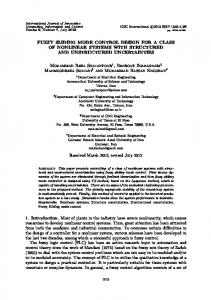
4. Application Examples The proposed control scheme was evaluated using an experimental application on the Scorbot robot system that is described in Figure 1, where only two links (“link1” for the upper arm and “link2” for forearm) were selected among the four links of the Scorbot robot manipulator. From (1),
6
Mathematical Problems in Engineering Table 1: Manipulator parameters. Symbol
Parameter
Quantity
𝑚1 , 𝑚2 𝐿 1, 𝐿 2
Mass of link1 and 2 Mass of link1 and 2 Stiction level of joint1 and 2 Coulomb friction of joint1 and 2 Stibeck velocity of joint1 and 2 Bristle stiffness of joint1 and 2 Presliding damping of joint1 and 2 Sliding damping of joint1 and 2
12.1 kg, 3.59 kg 0.3 m, 0.41 m
𝐹𝑠1 , 𝐹𝑠2 𝐹𝑐1 , 𝐹𝑐2 V𝑠1 , V𝑠2
Figure 1: Photograph of the Scorbot robot ERII system.
𝜎01 , 𝜎02
the dynamic parameters for two degree-of-freedom (DOF) links of the Scorbot robot manipulator are described as
M (q) = [
𝑀11 𝑀12 𝑀21 𝑀22
𝜎11 , 𝜎12 𝜎21 , 𝜎22
0.063 Nm, 0.0648 Nm 0.061 Nm sec/rad, 0.06 Nm sec/rad 0.00075 rad/sec, 0.00063 rad/sec 5400 Nm/rad, 8700 Nm/rad 5.4 Nm sec/rad, 6.2 Nm sec/rad 10.2 Nm sec/rad, 10.8 Nm sec/rad
],
𝑀11 = (𝑚1 + 𝑚2 ) 𝐿21 + 𝑚2 𝐿22 + 2𝑚2 𝐿 1 𝐿 2 cos (𝑞2 ) , 𝑀12 = 𝑚2 𝐿22 + 𝐿 1 𝐿 2 𝑚2 cos (𝑞2 ) ,
DC motor drive
A/D converter
Rotary encoder
Matlab RTI MF624 control board
𝑀21 = 𝑚2 𝐿22 + 𝐿 1 𝐿 2 𝑚2 cos (𝑞2 ) , 𝑀22 = 𝑚2 𝐿22 , −2𝑚2 𝐿 1 𝐿 2 sin (𝑞2 ) 𝑞2̇ −𝑚2 𝐿 1 𝐿 2 sin (𝑞2 ) 𝑞2̇ ], C (q, q)̇ = [ ̇ 𝑚 𝐿 𝐿 sin (𝑞 ) 𝑞 0 2 1 [ 2 1 2 ] 𝑚2 𝐿 2 𝑔 cos (𝑞1 + 𝑞2 ) + (𝑚1 + 𝑚2 ) 𝐿 1 𝑔 cos (𝑞1 ) ], G (q) = [ 𝐿 𝑔 cos (𝑞 + 𝑞 ) 𝑚 2 2 1 2 [ ] 𝜎01 𝑧1 + 𝜎11 𝑧̇1 + 𝜎21 𝑞1̇
], F𝑓 (q, q)̇ = [ ̇ ̇ 𝑧 𝜎 𝑧 + 𝜎 + 𝜎 𝑞 12 2 22 2 ] [ 02 2
D/A converter
(40)
where F𝑓 (q, q)̇ is the LuGre friction model [26]. Table 1 lists the chosen values of the link and actuator parameters. Three controllers were designed to evaluate the proposed control system: the conventional decentralized sliding mode controller (SMC) given in (33), the decentralized FTSMC given in (38), and proposed BSMC given in (27). The designed controllers were implemented on the MATLAB RTI system using an MF624 board [27]. The control signals were transferred to the DC servo motor of the Scorbot robot through the servo drive. The sample time was selected as 1 kHz. Figure 2 presents the schematic diagram of the control system. The sine-wave joint motion was chosen as the desired trajectory. The sine-wave position command was q𝑑 (𝑡) = 0.1 sin(2.5132𝑡) (rad). The controller parameters were 𝑐11 = = 0.01, 70, 𝑐12 = 2, 𝑐21 = 50, 𝑐22 = 2, 𝜂𝑓12 = 1, 𝜂𝑓22 = 1, 𝜂𝑓12
Figure 2: Diagram of the Scorbot robot control system.
𝜂𝑓22 = 0.1, 𝜂𝜌12 = 0.1, 𝜂𝜌22 = 0.1, 𝜂𝜌12 = 0.001, and 𝜂𝜌22 = 0.001. The tracking error performance functions were
𝜌1 (𝑡) = (0.2 − 0.005) 𝑒−4𝑡 + 0.005,
if 𝑒1 (0) < 0,
𝜌2 (𝑡) = (0.2 − 0.005) 𝑒−4𝑡 + 0.005,
if 𝑒2 (0) ≥ 0.
(41)
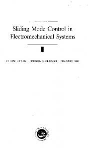
The initial points of each state were 𝑞1 (0) = −0.05 rad and 𝑞2 (0) = 0.05 rad. Figure 3 shows the tracking outputs of the SMC and the TFSMC, where the tracking performance of FTSMC improved slightly, compared to FSMC. Figures 4(a) and 4(b) show the tracking outputs of BSMC. The tracking errors of BSMC remained in the prescribed bound, whereas the tracking errors of SMC and FTSMC violated the prescribed bound as shown in Figures 4(c) and 4(d). The prescribed bound is satisfied if 0 ≤ |𝑒𝑖 (𝑡)| < 𝜌𝑖 (𝑡); that is, 0 ≤ |𝜉𝑖 (𝑡)| < 1. This property is shown in Figure 5(a). Figure 5(c) shows the estimated uncertainty of the RBF network approximation. The control inputs of each system are shown in Figure 6, where the proposed BSMC does not undergo severe chattering inputs unlike the FTSMC system. Therefore, the proposed BSMC could satisfy the given prescribed performance condition more effectively than the conventional SMC and FTSMC methods.
7
0.15
0.15
0.10
0.10
0.05
0.05 (rad)
(rad)
Mathematical Problems in Engineering
0.00
0.00
−0.05
−0.05
−0.10
−0.10
−0.15
−0.15
0
2
4
6
8
10
0
2
4
t (s)
6
8
10
8
10
8
10
t (s)
(a)
(b)
0.15
0.15
0.10
0.10
0.05
0.05 (rad)
(rad)
Figure 3: Position tracking outputs of the SMC (dashed) and FTSMC (solid): (a) link1. (b) link2.
0.00
0.00
−0.05
−0.05
−0.10
−0.10
−0.15
−0.15
0
2
4
6
8
10
0
2
4
t (s)
(a)
(b)
0.25
0.25
0.20
0.20
0.15
𝜌1(t)
0.15
FTSMC
SMC
0.10
SMC FTSMC
𝜌2 (t)
0.10
0.05
0.05 (rad)
(rad)
6 t (s)
0.00 −0.05
0.00 −0.05
BSMC
−0.10 −0.15
BSMC
−0.10
−𝜌1(t)
−𝜌2 (t)
−0.15
−0.20
−0.20
−0.25
−0.25
0
2
4
6
8
10
0
2
4
(c)
6 t (s)
t (s)
(d)
Figure 4: Position tracking results. (a) Tracking output of BSMC in link1. (b) Tracking output of BSMC in link2. (c) Tracking errors of SMC (dashed), FTSMC (dash-dot), and BSMC (solid) in link1. (d) Tracking errors of SMC (dashed), FTSMC (dash-dot), and BSMC (solid) in link2.
8
Mathematical Problems in Engineering 3
1.2 1.0
2
0.8 (Nm)
1 0.6 0.4
0
0.2
−1
0.0 −2 0
2
4
6
8
0
10
2
4
t (s)
6
8
10
6
8
10
6
8
10
t (s)
(a)
(a)
2
2.0
1
1.5
(Nm)
0 1.0
−1 0.5 −2 0.0 −3
0
2
4
6
8
0
10
2
4
t (s)
t (s)
(b)
(b)
1.5
1.0
1.0
0.8
0.5 (Nm)
0.6
0.4
0.0 −0.5
0.2
−1.0 −1.5
0.0 0
2
4
6
8
10
0
2
4
t (s)
t (s)
(c)
(c)
Figure 5: Position tracking results of BSMC: (a) 0 ≤ |𝜉1 | < 1 (solid) ̂𝑓1 (solid) and 𝑊 ̂𝑓2 . (c) 𝜎̂1 (solid) and 0 ≤ |𝜉2 | < 1 (dashed). (b) 𝑊 and 𝜎̂2 (dashed).
Figure 6: Control inputs. (a) Link1, SMC (dashed) and FTSMC (soild). (b) Link2, SMC (dashed) and FTSMC (solid). (c) BSMC, link1 (dashed) and link2 (solid).
Mathematical Problems in Engineering
5. Conclusion A BLF-based decentralized error-constrained SMC was developed to guarantee the position tracking performance of a robotic manipulator in the presence of unknown nonlinear dynamics. The error-transformed sliding surface was proposed to ensure the prescribed tracking error bound and to effectively compensate for the decentralizing uncertainty as well as the sliding condition. A prototype of the Scorbot manipulator demonstrated that the proposed BSMC scheme satisfies the prescribed tracking performance with RBF network approximation for an unknown nonlinear function. Therefore, the designed controller can have a simple structure and can more conveniently control the positioning function of robotic manipulator.
Acknowledgments This research was supported by the Ministry of Science, ICT and Future Planning (MSIP), Korea, under the Information Technology Research Center (ITRC) support program (NIPA-2013-H0301-13-2006) supervised by the National IT Industry Promotion Agency (NIPA).
References [1] R. M. DeSantis, “Motion/force control of robotic manipulators,” Transactions of the American Society of Mechanical Engineers, vol. 118, no. 2, pp. 386–389, 1996. [2] S. Chiaverini, B. Siciliano, and L. Villani, “A survey of robot interaction control schemes with experimental comparison,” IEEE/ASME Transactions on Mechatronics, vol. 4, no. 3, pp. 273– 285, 1999. [3] Z. P. Wang, S. S. Ge, and T. H. Lee, “Robust motion/force control of uncertain holonomic/nonholonomic mechanical systems,” IEEE/ASME Transactions on Mechatronics, vol. 9, no. 1, pp. 118– 123, 2004. [4] D. Zhao, X. Deng, and J. Yi, “Motion and internal force control for omnidirectional wheeled mobile robots,” IEEE/ASME Transactions on Mechatronics, vol. 14, no. 3, pp. 382–387, 2009. [5] A. Ilchmann, E. P. Ryan, and P. Townsend, “Tracking control with prescribed transient behaviour for systems of known relative degree,” Systems & Control Letters, vol. 55, no. 5, pp. 396– 406, 2006. [6] A. Ilchmann and H. Schuster, “PI-funnel control for two mass systems,” IEEE Transactions on Automatic Control, vol. 54, no. 4, pp. 918–923, 2009. [7] C. M. Hackl, “High-gain adaptive position control,” International Journal of Control, vol. 84, no. 10, pp. 1695–1716, 2011. [8] C. P. Bechlioulis and G. A. Rovithakis, “Robust adaptive control of feedback linearizable MIMO nonlinear systems with prescribed performance,” IEEE Transactions on Automatic Control, vol. 53, no. 9, pp. 2090–2099, 2008. [9] C. P. Bechlioulis and G. A. Rovithakis, “Adaptive control with guaranteed transient and steady state tracking error bounds for strict feedback systems,” Automatica, vol. 45, no. 2, pp. 532–538, 2009. [10] W. Wang and C. Wen, “Adaptive actuator failure compensation control of uncertain nonlinear systems with guaranteed transient performance,” Automatica, vol. 46, no. 12, pp. 2082–2091, 2010.
9 [11] J. Na, “Adaptive prescribed performance control of nonlinear systems with unknown dead zone,” International Journal of Adaptive Control and Signal Processing, vol. 27, no. 5, pp. 426– 446, 2013. [12] C. P. Bechlioulis and G. A. Rovithakis, “Robust partial-state feedback prescribed performance control of cascade systems with unknown nonlinearities,” IEEE Transactions on Automatic Control, vol. 56, no. 9, pp. 2224–2230, 2011. [13] K. P. Tee, S. S. Ge, and E. H. Tay, “Barrier Lyapunov functions for the control of output-constrained nonlinear systems,” Automatica, vol. 45, no. 4, pp. 918–927, 2009. [14] B. B. Ren, S. S. Ge, K. P. Tee, and T. H. Lee, “Adaptive neural control for output feedback nonlinear systems using a barrier Lyapunov function,” IEEE Transactions on Neural Networks, vol. 21, no. 8, pp. 1339–1345, 2010. [15] K. P. Tee and S. S. Ge, “Control of nonlinear systems with partial state constraints using a barrier Lyapunov function,” International Journal of Control, vol. 84, no. 12, pp. 2008–2023, 2011. [16] K. P. Tee, B. B. Ren, and S. S. Ge, “Control of nonlinear systems with time-varying output constraints,” Automatica, vol. 47, no. 11, pp. 2511–2516, 2011. [17] M. Kristic, I. Kanellakopoulos, and P. V. Kokotovic, Nonlinear and Adaptive Control Design, John Wiley & Sons, New York, NY, USA, 1995. [18] Y. Zhang, B. Fidan, and P. A. Ioannou, “Backstepping control of linear time-varying systems with known and unknown parameters,” IEEE Transactions on Automatic Control, vol. 48, no. 11, pp. 1908–1925, 2003. [19] J. E. Slotine and E. Li, Applied Nonlinear Control, Prentice Hall, Englewood Cliffs, NJ, USA, 1991. [20] C. J. Fallaha, M. Saad, H. Y. Kanaan, and K. Al-Haddad, “Sliding-mode robot control with exponential reaching law,” IEEE Transactions on Industrial Electronics, vol. 58, no. 2, pp. 600–610, 2011. [21] Y. Xiaofang, W. Yaonan, S. Wei, and W. Lianghong, “RBF networks-based adaptive inverse model control system for electronic throttle,” IEEE Transactions on Control Systems Technology, vol. 18, no. 3, pp. 750–756, 2010. [22] Y. Hong, Y. Xu, and J. Huang, “Finite-time control for robot manipulators,” Systems & Control Letters, vol. 46, no. 4, pp. 243– 253, 2002. [23] S. Yu, X. Yu, B. Shirinzadeh, and Z. Man, “Continuous finitetime control for robotic manipulators with terminal sliding mode,” Automatica, vol. 41, no. 11, pp. 1957–1964, 2005. [24] Y. Tang, M. Tomizuka, G. Guerrero, and G. Montemayor, “Decentralized robust control of mechanical systems,” IEEE Transactions on Automatic Control, vol. 45, no. 4, pp. 771–776, 2000. [25] M. Zhu and Y. Li, “Decentralized adaptive fuzzy sliding mode control for reconfigurable modular manipulators,” International Journal of Robust and Nonlinear Control, vol. 20, no. 4, pp. 472– 488, 2010. ˚ om, and P. Lischinsky, “A new [26] C. C. de Wit, H. Olsson, K. J. Astr¨ model for control of systems with friction,” IEEE Transactions on Automatic Control, vol. 40, no. 3, pp. 419–425, 1995. [27] Humusoft, MF 624 Multifunction I/O Card Manual, Humusoft, Prague, Czech Republic, 2006.
Advances in
Operations Research Hindawi Publishing Corporation http://www.hindawi.com
Volume 2014
Advances in
Decision Sciences Hindawi Publishing Corporation http://www.hindawi.com
Volume 2014
Journal of
Applied Mathematics
Algebra
Hindawi Publishing Corporation http://www.hindawi.com
Hindawi Publishing Corporation http://www.hindawi.com
Volume 2014
Journal of
Probability and Statistics Volume 2014
The Scientific World Journal Hindawi Publishing Corporation http://www.hindawi.com
Hindawi Publishing Corporation http://www.hindawi.com
Volume 2014
International Journal of
Differential Equations Hindawi Publishing Corporation http://www.hindawi.com
Volume 2014
Volume 2014
Submit your manuscripts at http://www.hindawi.com International Journal of
Advances in
Combinatorics Hindawi Publishing Corporation http://www.hindawi.com
Mathematical Physics Hindawi Publishing Corporation http://www.hindawi.com
Volume 2014
Journal of
Complex Analysis Hindawi Publishing Corporation http://www.hindawi.com
Volume 2014
International Journal of Mathematics and Mathematical Sciences
Mathematical Problems in Engineering
Journal of
Mathematics Hindawi Publishing Corporation http://www.hindawi.com
Volume 2014
Hindawi Publishing Corporation http://www.hindawi.com
Volume 2014
Volume 2014
Hindawi Publishing Corporation http://www.hindawi.com
Volume 2014
Discrete Mathematics
Journal of
Volume 2014
Hindawi Publishing Corporation http://www.hindawi.com
Discrete Dynamics in Nature and Society
Journal of
Function Spaces Hindawi Publishing Corporation http://www.hindawi.com
Abstract and Applied Analysis
Volume 2014
Hindawi Publishing Corporation http://www.hindawi.com
Volume 2014
Hindawi Publishing Corporation http://www.hindawi.com
Volume 2014
International Journal of
Journal of
Stochastic Analysis
Optimization
Hindawi Publishing Corporation http://www.hindawi.com
Hindawi Publishing Corporation http://www.hindawi.com
Volume 2014
Volume 2014