Batched Lazy Decision Trees
arXiv:1603.02578v1 [cs.LG] 8 Mar 2016
Mathieu Guillame-Bert and Artur Dubrawski Carnegie Mellon University School of Computer Science Pittsburgh, United States
[email protected],
[email protected] March 9, 2016
Abstract
Popular decision tree algorithms and more recently developed boosted and bagged decision tree algorithms are examples of eager algorithms that have been shown to be powerful state of the art methods. These algorithms build one or several decision trees, and use them as predictive models to process future queries. Such models may be computationally expensive to build but they are cheap to apply when trained. Friedman et al. [4] and later Fern and Brodley [6] experimented with the emulation of decision tree algorithms in lazy frameworks. These two approaches are respectively called a lazy decision tree and a boosted lazy decision tree. Unlike conventional (eager) decision tree algorithms, these approaches do not build full decision trees from training data but only explore a single path of the decision tree per unlabeled observation. While lazy decision trees can perfectly emulate operations of the conventional decision trees, Friedman et al. [4] and Fern and Brodley [6] have shown how using mutual information between training set and the unlabeled data during the decision tree building can improve the algorithm’s accuracy. The main drawback of lazy decision trees is their high computational cost in the prediction phase. They need to be re-run independently for each unlabeled observation. A potential solution to that problem is mentioned by Friedman et al. and it considers introducing of a caching scheme’. With this scheme, the algorithm remembers and re-uses the exploration paths traversed in previous runs. No details are available about this scheme. The authors only report that ”it consumes a lot of memory” [4].
We introduce a batched lazy algorithm for supervised classification using decision trees. It avoids unnecessary visits to irrelevant nodes when it is used to make predictions with either eagerly or lazily trained decision trees. A set of experiments demonstrate that the proposed algorithm can outperform both the conventional and lazy decision tree algorithms in terms of computation time as well as memory consumption, without compromising accuracy.
1
Introduction
In machine learning, the task of a classification algorithm is to predict the class label of an unlabeled observation, given an available collection of labeled training observations. Eager classification algorithms solve this task by building an intermediate explicit predictive model that can be then used to adjudicate the unlabeled observations. Conversely, non-eager classification algorithms (also called lazy classification algorithms) do not build an intermediate model. Instead, they compare the unlabeled observations to the whole set of training observations when making a prediction. As an example, ID3 decision tree and Random Forest [1] are eager algorithms, while k-Nearest Neighbours is an example of a lazy algorithm. 1
decision trees
In this paper, we introduce a lazy decision tree algorithm that exactly emulates the logic of eager decision trees and that solves the problem of unnecessary node exploration of both the conventional and lazy decision tree algorithms. The proposed algorithm is faster than eager decision trees, and therefore faster than lazy decision trees, while consuming the same amount of memory as a lazy decision tree (i.e. only one path through the tree is kept in memory at any instant) without the need for using memory-consuming caching schemes. We will refer to this algorithm as a batched lazy decision tree. Performance of the proposed algorithm is evaluated using bagging the models into ensembles of decision trees (bootstrap aggregation).
2
lazy decision trees batched lazy decision trees
1
1,4
2 3
5 4
A
6
B
1 2,5
7
A
3
B
2 6
A
3
B
4
Figure 1: Example of exploration of the same decision tree depending on the algorithm used. The example considers a training set without cached representation and two unlabeled observations A and B. The indices to the right of each node represent the sequences of exploration of the nodes (i.e. the step index of an algorithm). O(kmn log2 np ) and the time complexity of a lazy deciPlog n sion tree model is O( i=02 p m 2ni ) = O(mn2 ) on average. Note that log2 np is the average depth of exploration, 2i is the average number of nodes at depth i, and 2ni is the average number of training set observations contained in a node at depth i. Memory is rarely an issue when implementing decision trees but it deserves characterization. Building an eager decision tree requires memory for the stack operations used during the recursive construction of the tree as well as some storage for the final trained model. Lazy decision trees only require the stack. Using the same notation, the stack size and model size of decision trees are respecPlog n tively O( i=02 p 2ni ) = O(n) and O( np ) (i.e. number of non-leaf nodes in a decision tree) on average. Note that increasing the number of bootstrap samples in a bagged decision tree does not impact the stack size but just linearly increases the memory required to store the resulting trees. The stack size of lazy decision trees is O(n). Note that our analytic results assume that log2 np ≤ d where d is the maximum depth of exploration.
Decision trees and lazy decision trees
(Bagged) eager decision trees work by growing a set of non-pruned decision trees–each one trained on a bootstrapped set of reference observations. Listing 1 shows a generic bagged decision tree algorithm. A lazy decision tree emulates that operation by independently growing a single tree branch to handle each unlabeled observation. Listing 2 shows a generic bagged lazy decision tree algorithm. Since lazy decision trees only explore the branches used to predict unlabeled observations, they may end up exploring fewer nodes than exist in the equivalent conventional eager decision trees. This may happen if the test set is approximately just a subset of the data used for training the model. Nonetheless, lazy decision trees will repeat the exploration of some nodes. In practice, unless the number of unlabeled observations is small, lazy decision trees can be slower in prediction mode than the equivalent eager decision trees. Both algorithms are illustrated in Figure 1. We will now focus on the time and memory complexity of these algorithms. We consider a training dataset with n observations and m attributes. We assume the time complexity of evaluating an attribute is linear in the number of observations. Therefore, using a k-fold crossvalidation scheme and expanding nodes with a minimum of p training observations in them, the time complexity Plog n of an eager decision tree model is O( i=02 p 2i m 2ni ) =
3
Batched lazy decision trees
We will now introduce our batched lazy decision tree algorithm. We begin with the listing, and then discuss and compare batched lazy decision trees with the eager and lazy decision trees. Listing 3 shows the batched lazy decision tree algo2
Algorithm 1: Generic decision tree algorithm with bagging
Algorithm 2: Generic lazy decision tree algorithm with bagging input : T ∈ M nt ×(m+1) : The training set with n observations and m attributes. The last column contains the class labels. S ∈ M ns ×m : The testing set. b : Number of bootstraps. c : Minimum number of observations in a node (e.g. 5). d : Maximum depth (e.g. 20). output: R ∈ M ns ×h : The predicted probability for each class and each row of the testing dataset.
input : T ∈ M n×(m+1) : The training set with n observations and m attributes. The last column contains the class labels. b : Number of bootstraps. c : Minimum number of observations in a node (e.g. 5). d : Maximum depth (e.g. 20). output: R : A set of bagged decision trees. Algorithm R←∅ for i ← 1 to b do // For each bootstrap T 0 ← bootstrap rows of T R ← R ∪ {rec build(T 0 , 0)}
Algorithm for i ← 1 to b do // For each bootstrap T 0 ← bootstrap rows of T for j ← 1 to ns do // For each test observation X ← T0 d0 ← 0 while nrow(X) ≥ c and d0 ≤ d and X is not pure do a ← find the condition of X with the highest information gain d0 ← d0 + 1 if condition a is valid for the test observation j then X ← subset of X rows such that a is valid
0
Subroutine rec build(T 0 ∈ M n ×(m+1) ,i) if i > d or n0 < c or T 0 is pure then t ← create a node labeled with the most frequent class in T 0 return t a ← find the condition of T 0 with the highest information gain L ← subset of T 0 rows’ such that a is invalid R ← subset of T 0 rows’ such that a is valid tl ← rec build(L,i+1) tr ← rec build(R,i+1) t ← create a node with two children tl and tr , and labeled with a.
else X ← subset of X rows such that a is invalid f ← the most represented class in X Ri,f ← Ri,f + 1/b
rithm with bagging. Batched lazy decision trees behave similarly to lazy decision trees, however a lazy decision tree explores one path of inference going through it at a time. Since different test observations are likely to end up in different leaf nodes, lazy decision tree algorithm needs to be re-executed for each test observation. Batched lazy decision tree algorithm solves this issue by enabling the exploration of an arbitrary sub-tree instead of a single path. Batched lazy decision tree explores the same nodes as the regular lazy decision trees, however, each necessary node is visited only once through a single pass. Batched lazy decision trees will not visit nodes that are not used for the predictions. A diagram representation of a batched
lazy decision tree is shown in Figure 1. Note that the test data is never sorted in any way for the batched lazy algorithm. We only require the property that a test observation is being assigned to one and only one child of a given nonleaf node. The time complexity of batched lazy decision trees n P pi n n− n 2i (1 − (1 − 2−i ) k )( 2i k + ik2 ) = is O( i=0 3
Plog n n O(mn(log2 np − i=02 p (1−2−i ) k )). The computational complexity is difficult to characterize analytically, but it is strictly lower than the computational complexity of eager decision trees. The memory complexity is O(n), similar to that of lazy decision trees.
Table 1: Datasets used for the experimental evaluation.
Algorithm 3: Batched Lazy Decision Tree algorithm with bagging input : T ∈ M nt ×(m+1) : The training set with n observations and m attributes. The last column contains the class labels. S ∈ M ns ×m : The testing set. b : Number of bootstraps. c : Minimum number of observations in a node (e.g. 5). d : Maximum depth (e.g. 20). output: R ∈ M ns ×h : The predicted probability for each class and each row of the testing dataset. Algorithm for i ← 1 to b do // For each bootstrap T 0 ← bootstrap rows of T rec run(T 0 , S, 0)
Dataset
Rows
Columns
Rows/Cols
Size (kB)
C2U Breast Adult All Gamma
2695 569 32561 129 19020
212 31 15 12626 11
12.7 18.4 2 170 0.01 1 729
1139 118 1194 26780 1443
4
Empirical comparison
In this this section, we empirically evaluate the computational costs of eager, regular lazy, and batched lazy algorithms on five publicly available datasets–each dataset having different characteristics. Each algorithm is configured to compute b = 100 bootstraps, explore nodes with the minimum number of training data observations of p = 5 and a maximum depth of exploration of d = 20. Note that the computation complexities of all algorithms are linearly dependent to the parameter b. Also, both p and d limit the exploration capability of the tree. If log2 np < d, it is the p parameter that will mainly limit the exploratory behaviour. This constrain is true in all the tested datasets.
0
Subroutine rec run( T 0 ∈ M nt ×(m+1) , 0 S 0 ∈ M ns ×m , d0 ) if d0 > d or n0t < c or T 0 is pure then f ← the most frequent class in T 0 // For each test for j ← 1 to n0s do observation Rj,f ← Rj,f + 1/b
4.1
Datasets and implementation
We consider a diverse set of five benchmark datasets. Three popular UCI datasets [5] (Breast, Adult, and Gamma) and two medical genetic datasets (C2U [3] and ALL [2]). Table 1 reports various statistics for these sets. Informally, Breast, Adult, Gamma and C2U are small and average sized common type datasets, while ALL is a typical genetic dataset that contains many fewer observations than attributes. All three algorithms have been implemented in C++ and run on the same Intel-I7 computer equipped with 16GB of main memory. For accuracy of the results, the reported computation times are the sum of the user and kernel CPU times. All three algorithms rely on the same function to determine the best split of data at each node according to the information gain provided by each attribute.
return a ← find the condition of T 0 with the highest information gain Ls ← subset of S 0 rows such that a is invalid Rs ← subset of S 0 rows such that a is valid if Ls is not empty then Lt ← the subset of T 0 rows such the condition a is invalid rec run(Lt ,Ls ,d0 + 1) if Rs is not empty then Rt ← the subset of T 0 rows such the condition a is valid rec run(Rt ,Rs ,d0 + 1)
4
decision8trees lazy8decision8trees batched8lazy8decision8trees
Table 3: Number of memory words required to train one model in a 10-fold cross validation scheme for the eager decision tree (DT), the lazy decision tree (L-DT), and the batched lazy decision tree (BL-DT). Dataset C2U Breast Adult All Gamma
4.2
Stack
y=30081
Adult
Model
DT
L-DT
BL-DT
DT
15489 2562 214435 499 148078
4900 1036 89620 234 34582
11683 1934 170549 372 139098
312217 13000 1243262 3076 927200
ALL
Results
Figure 2 shows the computation times of k-fold crossvalidation for each algorithm and for various values of k, for each dataset. It also shows the average number of nodes explored by each of the considered algorithms. Table 2 shows the computation time that each method requires to process one fold in a leave-one-out crossvalidation scheme, i.e. the time needed to train the model and predict for a single test observation. Finally, table 2 reports the numerical values from Figure 2 for 10-fold and 40-fold cross-validation protocols. Table 3 shows the counts of memory words required to train and store (in the case of eager decision trees) one model built during a 10-fold cross-validation scheme. This table supposes that storing one observation index requires one word, and that storing one decision tree node requires four words (i.e. the attribute used, condition parameter, and addresses of the left and right sub-nodes). First, as Friedman et al. have suggested [4], we observed that lazy decision trees can be impractically slow. More precisely, lazy decision trees tend to require time during cross-validation when the number of folds is small in comparison to the number of observations. E.g. for the Breast dataset, lazy decision tree only becomes faster than an eager decision tree when the number folds exceeds 390. On this same dataset, we see that the lazy decision tree and our batched lazy decision tree are computationally equivalent for leave-one-out cross-validation. Additionally, both algorithms are faster than eager decision trees in this same setup. These last two observations
Breast
leave-1-out
y=340
C2U
y=42042
Gamma
Figure 2: Computation time and average number of explored nodes as a function of the number of crossvalidation folds.
are true on all datasets. We observe that batched lazy decision tree model is 5
Table 2: Computation time for one test observation (equivalent to the leave-one-out cross-validation protocol), 10fold, and 40-fold cross-validation for the eager decision tree (DT), the lazy decision tree (L-DT), and the batched lazy decision tree (BL-DT). Dataset Rows Columns CPU time of one observation CPU time of 10-folds CV CPU time of 40-folds CV C2U Breast Adult All Gamma
2695 596 32561 129 19020
212 31 15 12626 11
DT
L/BL-DT
Ratio
DT
L-DT
BL-DT
DT
L-DT
BL-DT
1.008 0.066 4.708 0.245 6.105
0.126 0.045 0.924 0.172 2.210
8.0 1.5 5.1 1.4 2.8
9.25 0.58 59.64 2.28 55.46
340.82 23.20 30 081 20.89 42 042
6.37 0.69 52.06 2.17 71.99
40.50 2.57 314.97 9.78 243.30
340.82 26.62 30081 22.15 42042
21.22 2.68 254.02 8.64 286.73
both the eager and lazy decision tree algorithms. W have conducted a set of experiments to evaluate empirically the time complexity of the proposed algorithm and its two contenders. These experiments have shown that the proposed algorithm is faster than both the conventional (eager, not-lazy) decision tree algorithms, and lazy decision tree algorithms – independently of the number of folds of data and the number of test observations. Finally, we characterized analytically and empirically the memory requirement of each algorithm. And we demonstrated that batched decision trees require significantly less memory that decision trees trained in standard ways.
strictly faster (Adult, All, C2U), equivalent (Breast), but it can also be slower (Gamma) than regular decision trees for less than a 100-fold cross-validation. In the Gamma dataset, we observe batched lazy decision tree becoming faster than alternatives for the number of folds higher than 350 (not shown in Figure 2). We see that the number of nodes explored by batched lazy decision tree is significantly lower that the number of nodes explored by eager or lazy decision trees. Interestingly, the drop in the number of explored nodes of a batched lazy decision tree in comparison to the eager decision trees is much greater than the computational time improvement. This phenomenon is due to the difference of computation cost of each node: Because of the variability of the number of available observations, nodes at the top of the tree (i.e. near the root) are more expensive to compute than nodes at the bottom of the tree (i.e. near the leafs). And, most of the node filtering of batched lazy decision trees happens at the nodes at the bottom of the trees. Finally, we observe that eager decision trees require significantly more stack memory than lazy decision trees, and at a somewhat smaller scale, also more than batched decision trees. Interestingly, we see that storing a bagged decision tree model requires significantly more memory than the stack space required for training the models.
[2] Sabina Chiaretti, Xiaochun Li, Robert Gentleman, Antonella Vitale, Franco Mandelli, Jerome Ritz, and Robin Foa. Gene expression profiles of b-lineage adult acute lymphocytic leukemia reveal genetic patterns that identify lineage derivation and distinct mechanisms of transformation. Clinical Cancer Research, 11(20):7209–7219, 2005.
5
[3] Michael Cummings and Daniel Myers. Simple statistical models predict c-to-u edited sites in plant mitochondrial rna. BMC Bioinformatics, 5, 2004.
References [1] Leo Breiman. Random Forrest. Machine Learning, 45(1):5–32, 2001.
Discussion
We introduced a lazy algorithm for decision trees. It solves the problem of unnecessary node exploration of
[4] J H Friedman, Ron Kohavi, Yeogirl Yun, and H Friedman. Lazy Decision Trees. In 13th National Con6
ference on Artificial Intelligence Conference (AAAI), AAAI’96, pages 717–724. AAAI Press, 1996. [5] M. Lichman. UCI machine learning repository, 2013. [6] Xiaoli Zhang Fern and Carla E. Brodley. Boosting Lazy Decision Trees. In Twentieth International Conference on Machine Learning, pages 178–185, 2003.
7