5 Jul 2011 ... 1 Introduction. Design of Experiments. The user experiment. 2 BLKs in the user
experiment. Analysis via BLKs. Utility functions. Optimal solution.
Introduction BLKs in the user experiment Conclusions and further work
Bayes linear kinematics in the design of experiments: the user experiment Kevin Wilson Newcastle University Supervised by Dr Malcolm Farrow and Dr Tom Nye
July 5, 2011
Kevin Wilson
BLK DoE
Introduction BLKs in the user experiment Conclusions and further work
1
Introduction Design of Experiments The user experiment
2
BLKs in the user experiment Analysis via BLKs Utility functions Optimal solution
3
Conclusions and further work Conclusions Further work
Kevin Wilson
BLK DoE
Introduction BLKs in the user experiment Conclusions and further work
Design of Experiments The user experiment
The choice of the design of an experiment can be viewed as a decision problem. There are trade offs between the costs of performing the experiment and the benefits derived from it. The benefits can be thought of in terms of gains in knowledge; either increase in information or some terminal payoff. The optimal design of an experiment is the best possible choice of design, found in a decision theoretic way.
Kevin Wilson
BLK DoE
Introduction BLKs in the user experiment Conclusions and further work
Design of Experiments The user experiment
� �
- P 1� � �� �� � � 6 θ ��
d1
? �� - X ��
- d2
Figure: The process of Bayesian experimental design Kevin Wilson
BLK DoE
Introduction BLKs in the user experiment Conclusions and further work
Design of Experiments The user experiment
The solution to the experimental design problem is the design which maximises the expected utility. In order to do this we specify a utility function. Utility function A utility function U is a means of expressing a decision maker’s preferences over the decision space.
Kevin Wilson
BLK DoE
Introduction BLKs in the user experiment Conclusions and further work
Design of Experiments The user experiment
If we have initial decision d1 , terminal decision d2 , unknown parameters θ, observed data x, and utility function U(d1 , d2 , θ, x) then for a design d1 the expected utility of the best decision is given by Z Z U(d1 ) = max U(d1 , d2 , θ, x)f (θ|x, d1 )f (x|d1 )dθdx, X d2 ∈D2
Θ
Optimal design The optimal design d1∗ maximises this: Z Z U(d1∗ ) = max max U(d1 , d2 , θ, x)f (θ|x, d1 )f (x|d1 )dθdx. d1 ∈D1
X d2 ∈D2
Θ
Kevin Wilson
BLK DoE
Introduction BLKs in the user experiment Conclusions and further work
Design of Experiments The user experiment
Thus the theory of Bayesian experimental design is ‘fairly’ straightforward. However, a full Bayesian analysis tends to be computationally difficult as only the simplest models allow integrals such as these to be solved analytically. Except in special cases neither the maximisation nor the the integration can be solved analytically and approximation and/or simulation based methods are needed. This means that solution of these problems is typically very computationally intensive and can quickly become infeasible.
Kevin Wilson
BLK DoE
Introduction BLKs in the user experiment Conclusions and further work
Design of Experiments The user experiment
Before software goes on sale or a website goes live testing is undertaken. One important aspect of this is to see whether the product is user-friendly. This is generally done by taking a sample of users and asking each to perform a number of tasks. From the results of these tasks usability problems with the software are identified and the software can either be launched as it is or rewritten. Kevin Wilson
BLK DoE
Introduction BLKs in the user experiment Conclusions and further work
Design of Experiments The user experiment
Sample size n
outcome
X=x Terminal decision
launch
rewrite Kevin Wilson
BLK DoE
Introduction BLKs in the user experiment Conclusions and further work
Analysis via BLKs Utility functions Optimal solution
If n users are asked to perform a task then the number who successfully complete that task, X , follows a binomial distribution X | θl ∼ bin(n, θl ), We shall make an exchangeability assumption; that users in the experiment and users who buy the product in the future are exchangeable. We are also interested in a second probability, θr . The two probabilities can be given marginal beta distributions θl ∼ beta(al , bl ), θr ∼ beta(ar , br ).
Kevin Wilson
BLK DoE
Introduction BLKs in the user experiment Conclusions and further work
Analysis via BLKs Utility functions Optimal solution
θl and θr will not in general be independent in our prior beliefs. First we transform; � � � � θl θr ηl = log , ηr = log , 1 − θl 1 − θr and then link ηl and ηr in a Bayes linear structure. Prior beliefs can be converted via E0 (θk ) =
ak ⇒ E0 (ηk ) = ψ(ak ) − ψ(bk ) ak + bk
and Var0 (θk ) =
ak b k ⇒ Var0 (ηk ) = ψ1 (ak ) + ψ1 (bk ) (ak + bk )2 (ak + bk + 1)
for k = l, r . We also need Cov0 (ηl , ηr ). Kevin Wilson
BLK DoE
Introduction BLKs in the user experiment Conclusions and further work
Analysis via BLKs Utility functions Optimal solution
Now, when X = x successes are observed θl is updated to θl | X = x ∼ beta(al∗ , bl∗ ), where al∗ = al + x and bl∗ = bl + n − x. This gives E(ηl | X = x) and Var(ηl | X = x). These updates can be propagated through to ηr via; E(ηr | X = x)
=
Var(ηr | X = x)
=
Cov0 (ηr , ηl ) [E(ηl | X = x) − E0 (ηl )] , Var0 (ηl ) � � Cov20 (ηr , ηl ) Var(ηl | X = x) Var0 (ηr ) − 1− . Var0 (ηl ) Var0 (ηl )
E0 (ηr ) +
The parameters of the posterior marginal beta distribution for θr can then be found by solving for ar∗ and br∗ ; E(ηr | X = x) = ψ(ar∗ ) − ψ(br∗ ),
Kevin Wilson
Var(ηr | X = x) = ψ1 (ar∗ ) + ψ1 (br∗ ).
BLK DoE
Introduction BLKs in the user experiment Conclusions and further work
Analysis via BLKs Utility functions Optimal solution
We shall also define Y , the number of customers who complete the task after the software has been released. Y ∼ bin(N, θk | X = x). The optimal terminal decision is E[U(topt | X = x)] = max{E[U(tl | X = x)], E[U(tr | X = x)]},
E[U(tk | X = x)] =
N Z 1Z 1 X y =0
0
0
U(sn , tk , Y , Ck )f (Y = y | X = x, θk )f (θl , θr | X = x)dθl dθr ,
for k = l, r . Then the optimal sample size is E[U(sopt )] = max{E[U(sn )]}, n ∈ N, where E[U(sn )] =
n X
f (X )E[U(topt | X = x)].
x=0 Kevin Wilson
BLK DoE
(1)
Introduction BLKs in the user experiment Conclusions and further work
Analysis via BLKs Utility functions Optimal solution
The probability that X = x is given by Z 1 f (X ) = 0
� f (X | θl )f0 (θl )dθl =
n x
�
Γ(al + bl ) Γ(al + bl + n)
Γ(al + x) Γ(bl + n − x) Γ(al )
Γ(bl )
Having made the update X = x the overall utility function U(sn , tk , Y , Ck ) depends only upon the chosen θ. Therefore one of the marginal adjusted beta distributions will always be sufficient to find the expected utilities. Thus E[U(tk | X = x)] =
N Z 1 X y =0
0
U(sn , tk , Y , Ck )f (Y = y | X = x, θk )f (θk | X = x)dθk ,
for k = l, r . Then
E[U(tk | X = x)]
=
� N Z 1� X Γ(ak∗ + bk∗ ) ak∗ −1 N b ∗ −1 y N−y θk (1 − θk ) × θ (1 − θk ) k dθk U() ∗ )Γ(b ∗ ) k y Γ(a 0 y =0 k k
=
� N � X Γ(ak∗ + bk∗ ) Γ(ak∗ + y ) Γ(bk∗ + N − y ) N U(sn , tk , Y , Ck ). ∗ ∗ y Γ(ak + bk + N) Γ(ak∗ ) Γ(bk∗ ) y =0
Kevin Wilson
BLK DoE
Introduction BLKs in the user experiment Conclusions and further work
Analysis via BLKs Utility functions Optimal solution
Design
Benefits
Costs
Experiment
No. successes
Per subject
Fixed Kevin Wilson
Rewrite
BLK DoE
Analysis via BLKs Utility functions Optimal solution
0.0
0.2
0.4
Utility
0.6
0.8
1.0
Introduction BLKs in the user experiment Conclusions and further work
0
20
40
60
80
100
Number of successes
The utility for the number of successes in N = 100 future customers in the task is given by y 1 − exp(− ) 10 . Us (Y ) = y 1 + 100 exp(− ) 10 Kevin Wilson
BLK DoE
Analysis via BLKs Utility functions Optimal solution
0.0
0.2
0.4
Utility
0.6
0.8
1.0
Introduction BLKs in the user experiment Conclusions and further work
0
50000
100000
150000
200000
Cost (£)
The utility for cost shall be � � 2Ck Uf (C ) = 1 − k log 1 + . Cmax Kevin Wilson
BLK DoE
Introduction BLKs in the user experiment Conclusions and further work
Analysis via BLKs Utility functions Optimal solution
If we assume mutual utility independence we can use a binary node U(sn , tk , Y , Ck ) = p1 Uf (C ) + p2 Us (Y ) + p3 Uf (C )Us (Y ). Suppose costs are Cmax = 200, 000, Cw = 50, 000, Co = 5, 000 and Cu = 500. Thus Cl = Co + Cu n = 5000 + 500n, and if the product is rewritten Cr = Co + Cu n + Cw = 55000 + 500n. We take p1 = 16 , p2 =
4 6
and p3 =
Kevin Wilson
1 6
BLK DoE
and, initially, N = 100.
Introduction BLKs in the user experiment Conclusions and further work
●
0.815
● ●
●
●
●
●●
Analysis via BLKs Utility functions Optimal solution
●● ●●
●
●
●
●
●
● ● ● ● ●
●
●
● ●
0.805
● ● ● ● ● ●
●
●
0.800
Expected Utility
0.810
●
●
● ● ●
●
● ●
0.795
● ● ● ● ● ●
0.790
● ● ●
●
0
10
20
30
40
50
Sample Size
Figure: A plot of E [U(sn )], the expected utility for each sample size
Kevin Wilson
BLK DoE
Analysis via BLKs Utility functions Optimal solution
0.2
Introduction BLKs in the user experiment Conclusions and further work
● ● ● ●
0.0
●
●
−0.2
Difference
●
●
−0.4
●
●
● ●
0
2
4
6
8
10
Number of Successes
Figure: The difference between the expected utilities of launch and rewrite with 11 users in the experiment Kevin Wilson
BLK DoE
Introduction BLKs in the user experiment Conclusions and further work
Conclusions Further work
Bayes linear kinematics reduces the computational burdens when solving problems in Bayesian experimental design. Issues of commutativity that are associated with Bayes linear kinematics were not a problem as a single update was made. Breaking down utilities into mutually independent utility hierarchies can aid in the specification of an overall utility function.
Kevin Wilson
BLK DoE
Introduction BLKs in the user experiment Conclusions and further work
Conclusions Further work
Extension of this approach to design of experiments to multiple updates. Discounting of future years in benefit utility. Defining a Bayes linear kinematic benefit utility in terms of information gain. Valencia poster!
Kevin Wilson
BLK DoE
Introduction BLKs in the user experiment Conclusions and further work
Kevin Wilson
Conclusions Further work
BLK DoE