Eastwood et al. SpringerPlus 2014, 3:55 http://www.springerplus.com/content/3/1/55
RESEARCH
a SpringerOpen Journal
Open Access
Bayesian hierarchical spatial regression of maternal depressive symptoms in South Western Sydney, Australia John G Eastwood1,2,3,4,5*, Bin B Jalaludin1,2, Lynn A Kemp1,2 and Hai N Phung1,2,5
Abstract Background: There is increasing interest in the role played by maternal depression in mediating the effects of adversity during pregnancy and poor infant outcomes. There is also increasing evidence from multilevel regression studies for an association of area-level economic deprivation and poor individual mental health. The purpose of the study reported here is to explore the spatial distribution of postnatal depressive symptoms in South Western Sydney, Australia, and to identify covariate associations that could inform subsequent multilevel studies. Methods: Mothers (n = 15,389) delivering in 2002 and 2003 were assessed at 2–3 weeks after delivery for risk factors for depressive symptoms. The individual-level binary outcome variables were Edinburgh Depression Scale (EDS) >9 and >12. The association between social, demographic and ecological factors and aggregated outcome variables were investigated using exploratory factor analysis and multivariate hierarchical Bayesian spatial regression. Relative risks from the final EDS >12 regression model were mapped to visualise the contribution from explanatory covariates and residual components. Results: The exploratory factor analysis identified six factors: neighbourhood adversity, social cohesion, health behaviours, housing quality, social services, and support networks. Variables associated with neighbourhood adversity, social cohesion, social networks, and ethnic diversity were consistently associated with aggregated depressive symptoms. Measures of social disadvantage, lack of social cohesion and lack of social capital were associated with increased depressive symptoms. The association with social disadvantage was not significant when controlling for ethnic diversity and social capital. Conclusions: The findings support the theoretical proposition that neighbourhood adversity causes maternal psychological distress and depression within the context of social buffers including social networks, social cohesion, and social services. The finding have implications for the distribution of health services including early nurse home visiting which has recently been confirmed to be effective in preventing postnatal depression. Keywords: Postnatal depression; Spatial epidemiology; Social capital; Social cohesion; Bayesian hierarchical regression; Exploratory factor analysis
* Correspondence:
[email protected] 1 Community Paediatrics, South Western Sydney Local Health District, Locked Mail Bag 7008, Liverpool BC 1871, New South Wales, Australia 2 School of Public Health and Community Medicine, The University of New South Wales, Sydney, NSW 2052, Australia Full list of author information is available at the end of the article © 2014 Eastwood et al.; licensee Springer. This is an open access article distributed under the terms of the Creative Commons Attribution License (http://creativecommons.org/licenses/by/2.0), which permits unrestricted use, distribution, and reproduction in any medium, provided the original work is properly cited.
Eastwood et al. SpringerPlus 2014, 3:55 http://www.springerplus.com/content/3/1/55
Background There is increasing interest in the role played by maternal depression in mediating the effects of adversity during pregnancy and poor infant outcomes. There is also increasing evidence from multilevel regression studies for an association of area-level economic deprivation and poor individual mental health (Fone et al. 2007; Skapinakis et al. 2005; Weich et al. 2003). Perinatal depression has consistently been found, at the individual level, to be higher among women with low socio-economic status (Beck 2001; O’Hara and Swain 1996). This raises the possibility that the impact of economic and social deprivation on mothers and their infants may be mediated through perinatal depression. With the exception of an area-level study of poverty and postpartum psychosis (Nager et al. 2006) we found no previous published ecological or multilevel studies of perinatal depression. We have previously reported on individual level psychosocial predictors of perinatal depression in South Western Sydney (SWS) and proposed that the findings were consistent with group-level socioeconomic deprivation, neighbourhood environment, social capital and ethnic diversity having causal effects on postnatal depressive symptomatology and other perinatal outcomes (Eastwood et al. 2011). That proposition is consistent with a recent qualitative study of pathways from neighbourhoods to mental well-being which found that neighbourhood affordability, negative community factors including crime and vandalism, and social makeup including unemployment and poverty, were associated with poor mental wellbeing (O’Campo et al. 2009). The study reported here uses Bayesian hierarchical modelling techniques to explore spatial relationships between aggregated postnatal depressive symptoms and potential ecological covariates identified in a preceding qualitative study (Eastwood et al. 2014a, Eastwood et al. 2014b). Unlike conventional statistical inference which derives the average estimates of parameters, hierarchical Bayesian modelling produces parameter estimates for each individual analysis unit by borrowing information from all other analysis units (Zhu et al. 2006). Likelihood ordinary least squares (OLS) linear regression treats each suburb in isolation so that there is no recognition in the model of the spatial relationships that may exist between suburbs and therefore no modelling of spatial variability (Law and Haining 2004). To address this problem Law and Haining (Law and Haining 2004) proposed fitting random effects models where the random variation is spatially structured. A key feature of Bayesian spatial regression models is that they incorporate such random spatial effects into the modelling of outcome and covariate effects at the ecological level. These random spatial effects may reflect unmeasured confounders and thus the model makes it possible
Page 2 of 10
to ascertain whether the residual effects suggest spatial patterns or clusters (MacNab 2004). The study reported here is part of a larger multilevel research programme that utilises critical realist mixed qualitative and quantitative methodology to build a theoretical model of the mechanisms by which multilevel factors might influence the developmental origins of health and disease (Eastwood et al. 2014c). The aim of this study is to explore the spatial distribution of perinatal depressive symptoms in South Western Sydney and to identify any associations that can inform subsequent multilevel studies, theory building and local public health interventions.
Methods Study design
The analysis reported here is part of an exploratory ecological study of aggregated rates of postnatal depressive symptoms in South Western Sydney Area Health Service from 2002–2003. The aggregated rates used in this study were derived from an individual-level cross-sectional study of mothers of infants born in South Western Sydney Area Health Service (SWSAHS) from 2002 to 2003 (Eastwood et al. 2012a). That study (n = 15,389) was a sub-sample from a larger dataset collected from 1998 to 2006. A 2004 to 2006 subsample was retained for subsequent confirmatory studies. The main study included: individual level logistic regression (Eastwood et al. 2012a) and non-linear principal component analysis (Eastwood et al. 2012b); group-level visualisation of maps of co-variants, cluster analysis (Eastwood et al. 2013a), exploratory factor analysis (Eastwood et al. 2013b, Eastwood et al. 2014a), ecological likelihood and Bayesian spatial linear regression (Eastwood et al. 2013b); and Bayesian spatial multi-level analysis. The decomposed results of the Bayesian spatial linear regression are reported here using the findings for the previously reported EFA to assist interpretation. Study setting
The setting is all suburbs in four local government areas (LGAs) south-western Sydney, New South Wales (NSW), Australia. The individual-level data available for study was coded by suburb of residence. The suburb of residence was chosen as the closest group-level administrative unit to naturally occurring local neighbourhood environments. There were 101 suburbs available to study using the 2001 Census maps. Participants
As previously reported the main study utilised the Ingleburn Baby Information System (IBIS) database. That database was initiated in 1995 and is based on the routine survey by Child and Family Health Nurses of
Eastwood et al. SpringerPlus 2014, 3:55 http://www.springerplus.com/content/3/1/55
all mothers who attend the first well baby clinic (home visit or clinic based) after discharge from the postnatal ward. Population-based collection started in Campbelltown and Wollondilly in 1998, followed by Bankstown in 2000, Fairfield and Wingecarribee in 2001 and Liverpool in 2002. The calendar years of 2002 and 2003 were used for this study as all geographical areas, and 92% of births (n = 21,991) were surveyed. Of those surveyed 70 percent consented to completing an EDS and were included in this analysis. The mothers who did not complete an EDS were more likely to report: difficult financial situation, public housing accommodation, low maternal education, not breast feeding and short suburb duration. We have reported previously on the systematic nature of the missing data in the 2002 to 2003 subsample used for our exploratory studies (Eastwood et al. 2012a). Outcome variable
The outcome variable used for this study is the Edinburgh Depression Scale (EDS) (Cox et al. 1987), which has been widely used to study individual maternal perinatal depressive symptoms. This study reports on group level aggregation of two individual-level binary outcome variables, namely for EDS > 9 and EDS > 12 (Eastwood et al. 2012a). The use of EDS > 9 and EDS > 12 are supported by previous studies as screening cut-off points in English-speaking populations (Cox et al. 1987; Buist et al. 2002). Buist et al. (2002) noted that using EDS > 12 was a sound option for reducing false positive diagnosis of depressive illness. The original authors recommended using the EDS > 9 as a community screening cut-off point as many women experiencing considerable dysfunction, but not meeting diagnostic criteria for formal illness, might otherwise be missed. Those women also merit recognition of their distress and the provision of psychological or social assistance (Buist et al. 2002; Brown et al. 2001). Covariates
As previously reported (Eastwood et al. 2013b, Eastwood et al. 2014a), the selection of group level variables for analysis was principally influenced by concepts emerging from interviews with experienced maternal and child health practitioners, group interviews with mothers of infants and latent variables identified in individual level nonlinear principal component analysis (Eastwood et al. 2012b). The domains assessed as measurable at the suburb level were: social networks, capital and cohesion; “depressed community”, health behaviours, access to services and ethnic segregation or integration. 2001 Census data were used for the majority of the group level candidate variables. NSW crime statistics and aggregated individual level study data were also used. Areal data that was not available at the suburb
Page 3 of 10
level could not be used for the analysis reported here. Forty six variables were selected as candidate variables and have been previously described (Eastwood et al. 2013b, Eastwood et al. 2014a). A table summarising the 46 variables is available as an on-line supplement to this paper (Additional file 1: Table S1). Selected variables are described here to aid interpretation. The Index of Relative Socioeconomic Disadvantage (IRSD) is a composite index that contains indicators of disadvantage such as low income, high unemployment and low levels of education. The IRSD reflects lack of disadvantage rather than advantage and a high score implies than an area has few families with low income, few people with little or no training and few people working in unskilled occupations (ABS 2001). For concepts such as social cohesion and social capital there were no candidate variables in the 2001 Census data. Voluntary work was used from the 2006 Census. Social capital questions from the NSW Health survey were only available at local government level. We therefore used the aggregated IBIS variables “social support” and “no regret leaving [the] suburb”, while acknowledging the possibility of same-source bias as identified by Radenbush and others (Duncan and Raudenbush 1999; Radenbush and Sampson 1999) cited by (O’Campo 2003). As previously observed the multicultural nature of the population of the study area and themes emerging from the qualitative studies necessitated the selection of measures of ethnic diversity (Eastwood et al. 2013a, Eastwood et al. 2013b, Eastwood et al. 2013c, Eastwood et al. 2014a, Eastwood et al. 2014b). Three measures of ethnic diversity were selected based on the advice given to the US Bureau of the Census by Galster 2004. They were the: Maly Neighbourhood Diversity Index (Maly 2000), Entropy Index (Modarres 2004) and the Simpson’s Index (Simpson 1949). The Maly (neighbourhood diversity) index ranches from 0 – 1 where a suburb is: 0 with a completely homogeneous ethnic group and, 1 with a completely heterogeneous distribution which matches the metropolitan distribution. The Simpson and Entropy indexes are similar with 0 being completely homogenous and 1 being completely heterogeneous distribution of ethnic groups. The qualitative interviews also drew attention to the possible importance of extremes of wealth and poverty within neighbourhoods. As previously reported (Eastwood et al. 2013b, Eastwood et al. 2014a), we used here the Index of Extremes (ICE) which is computed as the number of affluent families in Census tract minus the number of poor families, divided by the total number of families in the Census tract (Massey 2001; Casciano and Massey 2008). The index varies from a theoretical minimum of −1.0 (all families are poor) to a theoretical maximum of +1.0 (all families are affluent) and passes through 0 (affluent and poor are equally balanced).
Eastwood et al. SpringerPlus 2014, 3:55 http://www.springerplus.com/content/3/1/55
Statistical analysis
Forty six candidate variables (Additional file 1: Table S1) were analysed using correlation matrices, univariate likelihood OLS linear regression, and factor analysis related diagnostic tests of multi-collinearity. Examination of the initial correlation matrices identified variables that were highly correlated and some were mutually exclusive. For example “different address five years previously” and “same address five years previously”. Of the initial 46 variables 31 were selected for EFA following the initial analysis. The EFA then commenced with a serious of further diagnostics as described below. At the completion of the diagnostics the number of variables entered into the EFA had been reduced to 26. Factor analysis
As observed above the aim of the main study was theory building. For theoretical EFA where there is expected to be correlation between factors the most appropriate method of extraction is “common factor analysis” as opposed to principal component analysis. As previously reported we used principal-axis factoring with oblimm oblique rotation. We also compared the solution with outputs from Principal Component Analysis (PCA) and EFA with orthogonal rotation. The extracted factors were in all cases the same. The initial correlation matrix was examined for high correlations among variables. Bartlett’s test, the KaiserMeyer-Olkin measure, and examination of the anti-image matrix were also used to evaluate whether the correlation matrix was suitable for factor analysis. Communalities that loaded less than 0.50 were also analysed. We generated a scree plot to determine the adequate number of components to retain in the analysis. After comparing extractions of 5, 6, 7 and 8 solutions, a 6 factor solution was selected as the best in terms of interpretability. The exploratory factor analysis enabled identification of multi-colinearity among the candidate covariates, assisted in the selection of variables for analysis in the spatial regression models and identified underlying latent variables for subsequent theory building. Bayesian modelling EDS
The Bayesian modelling strategy was to first fit a lognormal model for relative risk using observed and expected counts for both of the outcome variables EDS > 9 and EDS > 12. The expected count for each suburb was computed using the observed EDS > 9 or EDS > 12 rates for the South Western Sydney region multiplied by the number of mothers surveyed in that suburb. The number of women surveyed in each suburb may not have represented the true distribution of women who might have been surveyed. We therefore also undertook standardisation using “women of child bearing age”
Page 4 of 10
(WCBA). The rates standardised by numbers surveyed was highly correlated with the standardisation by WCBA and we therefore used the numbers surveyed. This basic log-normal model allowed for subsequent covariate adjustment, for spatial correlation of risk in nearby areas and for the addition of unstructured variance terms. This ‘Besag, York and Mollie’ (BYM) model for relative risks, (Besag et al. 1999) takes into account the effects that vary in a structured manner in space (clustering or correlated heterogeneity) and a component that models the effects that vary in an unstructured way between areas (uncorrelated heterogeneity) (Lawson et al. 2003). The conditional autoregressive (CAR) component used data from an adjacency matrix for the study area which was generated using the Adjacency Tool in GeoBUGS 1.1 (Spiegelhalter et al. 2003). We used the map decomposition strategy developed by Law and Haining (Law and Haining 2004) to visualise the results of the best fitting models. The map decomposition method allows separate mapping of the contribution made by the explanatory covariate variables, spatial clustering and heterogeneity (see Additional file 2: Table S2 for the WinBUGS code). Each covariate was fitted separately and model fit was assessed using changes in deviance information criterion (DIC). We also report the pD which is the number of effective parameters in the model. Smaller values of DIC indicate better fitting models. To compare DIC values, we carried out several runs using different initial values and random-number seeds (Spiegelhalter et al. 2002). Based on the results, we chose to distinguish between models where the DIC varied by more than one. Significance was assessed as non-zero regression coefficients at 95% credible interval. The covariate, that when added, resulted in the largest decrease in DIC was then analysed together with each of the remaining covariates. The process was repeated by adding further covariates until the DIC could be reduced no further. The final model(s) are reported. The specification of priors for the parameters is important in Bayesian inference. There have been no previously reported Bayesian studies of postnatal depressive symptoms; and therefore for the intercept we used a “vague” prior with a normal distribution, a mean of zero and large variance N(0, 10 000). For the precision of the random effects we used the commonly used hyper-prior of Gamma (0.5, 0.0005) as recommended by Kelsall and Wakefield (Kelsall and Wakefield 2002). For the variance we used an inverse Gamma prior. Sensitivity analysis was undertaken. All models assessed were run using two chains simultaneously. Convergence had occurred by 3,000 iterations in all cases. Each chain was then run for a further 3,000 iterations, with acceptable Monte Carlo (MC) errors.
Eastwood et al. SpringerPlus 2014, 3:55 http://www.springerplus.com/content/3/1/55
These samples were used to generate the posterior distributions from which the estimates of the parameters were obtained. The exploratory factor analysis was undertaken using SPSS 17.00. All Bayesian analysis was undertaken in WinBUGS 1.4 (Spiegelhalter et al. 2003). The posterior relative risks were mapped using ArcGIS 3.2 (Environmental Systems Research Institute 2008).
Page 5 of 10
Table 1 Factor analysis oblique rotation output – pattern matrix Factors 1 One Parent Families%
.818
Public Housing%
.777
Unplanned Pregnancy%
.709
Ethics approval
Occupational Class 3%
.584
The study obtained ethics approval from the Human Research Ethics Committee, South Western Sydney Area Health Service and from the University of NSW Human Research Ethics Committee.
Poor Families%
.567
Violent Crime rate
.546
Exploratory factor analysis (EFA)
We have previously reported the results of the factor analysis (Eastwood et al. 2013b, Eastwood et al. 2014a). The pattern matrix factor loadings obtained are shown in Table 1 to assist the later theoretical analysis of the Bayesian spatial regression. The factor loadings arranged in decreasing order within factors and with loadings less than 0.30 suppressed to aid interpretation. Based on the loadings in Table 1 we have here called Factor 1 – disadvantaged community; Factor 2 – Social Cohesion; Factor 3 - Health Behaviours; Factor 4 - Housing Quality; Factor 5 – Access to Services; and Factor 6 – Social Capital. Spatial linear regression (Bayesian)
We first fitted a log-normal model followed by models with uncorrelated and correlated components. Models with only spatial random effects were the best fit closely followed by the full ‘Besag, York and Mollie’ (BYM) model. We then fitted every candidate variable using the spatial random effects model. Table 2 shows the effective number of parameters in the model (pD) and the Deviance Information Criteria (DIC) results for models with: intercept only, correlated and uncorrelated residuals, full BYM, and a representative set of covariates. Best fitting spatial models
The multivariate EDS > 9 model with the lowest DIC and no non-significant coefficients included the covariates:% No Social Support, Entropy Index,% Apartments and% Smoking (Table 3). Models that included:% No Regret Leaving and% One Parent Families also performed well. The multivariate EDS > 12 models with the lowest DIC and no non-significant coefficients included:% No Social Support, Entropy Index, and either% No Regret Leaving or % Smoking (Table 3). There were no other models with three covariates where the coefficients were significant.
3
4
-.437
.927
Entropy Index
-.784
-.307
No volunteerism%
-.651
.305
Low Schooling%
-.567 -.468
-.406
.528
Breast feeding%
.907
Smoking%
.899
No Regret Leaving%
.795
Apartments% Single Houses%
-.825 -.427
.728
Vacancy Rate
-.637
Nurse Visit Rate
.405
Home Visit Rate Poor Health%
6
-.360
Volunteerism%
IRSD Decile
5
.912
Rented Dwellings%
Results
2
.767 .535
.304
.363
No Social Support%
-.679
No Practical Support%
-.589
Density
-.452
Different address last 5 years Maly Index
-.493 .349
.395 .308
Extraction method: principal axis factoring. Rotation method: oblimin with Kaiser Normalization.
We have elected to report here in more detail the best fitting of the aggregated EDS > 12 models namely that including the covariates:% No Support, Entropy Index and “%No Regret Leaving”. Table 4 shows the summary posterior parameters for the final EDS > 12 BYM model. Table 5 shows the posterior Odds Ratio for the final EDS > 12 BYM model. The odds of EDS > 12 was increased in suburbs with increased percentage of “no support” and percent “No Regret Leaving”. The odds was also increased in suburbs with a high Entropy Index. Map decomposition of the full BYM model enables visualisation of the full range of posterior estimated relative risks and residuals. This approach allows high and low areas of relative risk to be identified as well as an assessment of the contribution made by the covariates, unstructured and spatially structured random effects.
Eastwood et al. SpringerPlus 2014, 3:55 http://www.springerplus.com/content/3/1/55
Page 6 of 10
Table 2 Comparison of DIC for selected covariates in univariate spatial models EDS > 9
EDS > 12
Table 3 Best fitting spatial CAR regression models Models
Pd
DIC
EDS > 9 Best Fitting CAR Models
Variable
pD
DIC
pD
DIC
No Covariate CAR Model
23.404 565.468
Intercept Only
1.001
601.734
0.981
502.008
No Support
15.907 560.012
+ uncorrelated residual
28.285
580.712
21.814
487.733
No Support + Entropy
13.012 558.326
+ spatial residual (CAR)
23.623
565.503
21.957
473.102
No Support + Entropy +%Apartment
12.373 554.417
+ spatial + uncorrelated residual
26.185
567.673
23.887
475.944
No Support + Entropy +%Apartment + nurse visit rate
10.449 555.714
No Support + Entropy +%Apartment +%No regret leaving
10.146 554.072
No Support + Entropy +%Apartment +%One Parent Families
9.296
No Support + Entropy +%Apartment +%Smoking
10.543 552.535
CAR with covariates One Parent Family%
23.082
565.160
18.677
472.724
Rented Dwelling%
23.162
564.836
17.747
472.030
Unplanned Pregnancy%
18.828
561.784
13.814
470.470
Poor Families%
21.602
564.252
15.218
471.154
Volunteerism%
15.460
561.749
13.158
468.012
Entropy Index
17.593
564.483
14.551
469.984
Low Schooling%
18.680
562.840
15.848
471.488
IRSD Decile
13.635
564.481
7.529
472.089
Breastfeeding%
22.781
565.391
19.899
473.967
No Regret Leaving%
18.237
562.061
13.800
465.737
Apartments%
24.575
566.794
17.558
471.806
Nurse Visit Rate
25.430
567.276
22.230
475.631
No Social Support%
15.907
560.012
11.433
466.878
Maly Index
23.994
564.131
19.074
470.150
Density
18.318
561.917
15.545
470.901
Legend: EDS (Edinburgh Depression Scale), IRSD (Index of Relative Social Deprivation), CAR (Conditional Autoregression), pD (Effective number of parameters in the model), DIC (Deviance Information Criteria).
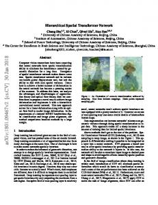
Figure 1 shows the map of Relative Risk for EDS > 12 in the final BYM model. Clustering of EDS > 12 can be seen in the northern suburbs in the “basic” CAR model. The relative risks (RRs) for areas in the north are strongly driven by the covariates “% No Social Support”, and Entropy. The covariate% No Regret Leaving is making a contribution to the RR in several other areas of the map. The maps of the residuals are strongly dominated by the unexplained spatial residual which is strongest in the southern suburbs.
Discussion The analysis presented here has identified suburbs in South Western Sydney where rates of maternal depressive symptoms are higher than expected for the region as a whole. We know from previous spatial studies of South Western Sydney (Phung et al. 2003) that those same communities have higher rates of social disadvantage and non-English speaking populations. Our qualitative studies also indicated that maternal depressive symptoms would be higher in communities with weak social networks, capital or cohesion; “depressed community”, poor access to services and ethnic segregation.
553.803
No Support + Entropy +%Apartment +%Smoking (BYM) 12.340 553.200 EDS > 12 Best Fitting CAR Models No Covariate
21.481 473.277
No Support
11.433 466.878
No Support + Entropy
10.352 462.743
No Support + Entropy + Smoking
7.997
460.240
No Support + Entropy + No Regret Leaving Suburb
9.208
459.622
Figure 1a shows the RRs for EDS > 12 in a model with no covariates. Clustering of EDS > 12 can be seen in the north eastern and north western suburbs. The pattern in the final BYM model is different with high RRs in more central suburbs of the northern region and in a few southern suburbs. The map decomposition indicates which of the covariates contribute to the ecological risk of depressive illness and in which suburbs. The RRs for areas in the north are strongly driven by the covariates “% No Support” and Entropy, while the covariate% No Regret Leaving is making a contribution to the RRs in several other areas of the map. The covariate% No Support is an aggregate variable of no support network at the individual level. We consider that this variable, and Factor 6 on which it loads, represents the latent variable social capital at the suburb level. The Entropy Index is a measure of ethnic diversity which loaded on Factor 2. In this study it is associated with a latent variable (F2) which may represent social cohesion. In the factor analysis, social cohesion was only Table 4 Summary statistics for parameters in BYM model EDS >12 Node
Mean
Intercept
−0.098 0.037
sd MC error 2.50% Median 97.50% −0.098
−0.026
No Support
0.074 0.035
0.001
0.000 −0.171 0.004
0.074
0.142
Entropy Index
0.112 0.047
0.001
0.021
0.112
0.205
No regret leaving
0.143 0.057
0.001
0.030
0.144
0.253
Legend: sd (standard deviation), MC (Monte Carlo).
Eastwood et al. SpringerPlus 2014, 3:55 http://www.springerplus.com/content/3/1/55
Page 7 of 10
Table 5 Posterior expected odds ratio for BYM model EDS > 12 Node
Mean
sd
MC 2.50% Median 97.50% error
OR.%No Support
1.08 0.04
0.00
1.00
1.08
1.15
OR. Entropy Index
1.13 0.05
0.00
1.03
1.13
1.23
OR.%No Regret Leaving
1.15 0.07
0.00
1.03
1.15
1.28
Legend: sd (standard deviation), MC (Monte Carlo).
slightly correlated with social capital (r = 0.26). The spatial distribution (not reported here) of the factors is also different. Together with the spatial regression analysis reported here, these findings support the proposition that social cohesion and social capital are independent latent variables that are negatively associated with aggregated rates of depressive illness. The variable “no regret at leaving the suburb” has been used in previous studies as an indicator of social cohesion (NSW Department of Health 2006). In our study,
Figure 1 Posterior expected relative risks (BYM model) for EPDS > 12. (a) EDS > 12 Bayesian CAR; (b) Ecological BYM Regression; (c) Entropy fixed effect; (d) No support fixed effect; (e) No regret leaving fixed effect; (f) spatial unexplained component; (g) unstructured unexplained component.
Eastwood et al. SpringerPlus 2014, 3:55 http://www.springerplus.com/content/3/1/55
this variable is correlated with community norms of smoking and not breastfeeding and not related to either social cohesion or social capital. In the EFA correlation matrix, health behaviours (F3) was moderately correlated with disadvantaged community (r = 0.4) suggesting that suburbs with poor “health behaviours” were also likely to be disadvantaged. Interestingly, there were no variables from Factor 1 representing the possible latent variable of “disadvantaged community” in the final EDS > 12 model. One of the final EDS > 9 regression models included% One Parent Families. The univariate spatial regression identified variables loading on Factor 1 as significantly associated with aggregated depressive symptoms, including: Index of Relative Social Deprivation (IRSD),% Occupation Class 3,% unemployed,% One Parent Families,% poor families and Index of Concentrated Extremes (ICE). When controlling for entropy and% no support in the EDS > 12 model, these variables were no longer significant. Aneshensel (2009) notes that distal factors, such as income, are often not statistically significant when more proximal factors, such as social support, are taken into consideration. The findings here would be consistent with the latent variable disadvantaged community, and its associated observed variables, being distal to social cohesion and social capital on a causal pathway as proposed by Carpiano (2006). The maps of the residuals are strongly dominated by the unexplained spatial component which is strongest in the southern suburbs. The implication of this is that a covariate that would remove this spatial residual has not been included in the model. It is also possible that such a covariate was not identified among the candidate variables included in this study. The study reported here was of all mothers giving birth in 2002 to 2003. The spatial residuals may also represent a sub-group of mothers who are at higher risk when living in the southern suburbs where social support networks are strong. The findings of the spatial regression could be interpreted as suggesting that mothers were more likely to have depressive symptoms if they live in communities with low social support networks, ethnic diversity (heterogeneity) and populations who would have “no regret leaving”. Based on the factor analysis loading of these three variables the findings suggest that women are more likely to be depressed if they live in communities with low social capital, low social cohesion and community-level unhealthy behaviours (which are associated with disadvantaged communities). Methodological matters
As we have previously observed (Eastwood et al. 2012a), that the size (15,389) of this cross-sectional study of the EDS administered to postnatal women is unique. There
Page 8 of 10
have been few previous reports of postnatal depression studies on population samples of this order. We have also previously reported on the limitations of the crosssectional design for causal inference and the impact on generalizability of sample selection bias from refusal and non-response in the study population. Importantly not all households with births in the study period were surveyed. That would have included mothers who had lost infants. The households not questioned with the IBIS questionnaire included mothers who moved to “out of area” locations or mothers who declined the nurse firstvisit offered. Also missing may have been some infants in intensive care units. Observational (information) bias may have been present in the survey data. This could have arisen from recall bias, or interviewer/responder bias. A particular problematic feature of self-reporting surveys is the mental state of the subject. Depressed women are more likely to have a negative view of their circumstances. This must be taken into account when considering the association found in this study of high EDS with subjective variables such as “rating of own health”, “reluctance to leave the suburb”, and “difficult financial situation”. The EDS is administered in English or via an interpreter where the mother is non-English speaking (NESP). We were not able to report in this study on the percentage of NESP mothers in the full sample but the percentage of NESP mothers in the Local Government Areas of Fairfield, Campbelltown, Camden and Wollondilly (linked data) was 11.8 percent at the time of the 2001 Census. This may be an important source of information bias in this study. Specific non-English EDS are not currently used postpartum in SWS but could be considered for future use. The limitations of ecological studies in making inferences regarding individual-level associations based on group-level data are well established (Greenland 1992). The findings reported in this study could reflect a compositional effect reflecting the aggregated characteristics of women (and possibly their partners) with depressive symptoms. Multilevel studies enable the simultaneous examination of the effects of group level and individual level variables on individual level outcomes (Duncan et al. 1995). Causal inference would be assisted by such an approach. The strength of the current study is the use of Bayesian hierarchical approaches to spatial autocorrelation thus addressing the limitations of linear methods which treat each suburb as being independent of surrounding suburbs. The map decomposition strategy developed by Law and Haining (2004) proved useful and in particular raised questions regarding the spatial distribution of unexplained components. Bayesian methods are increasingly being used in multilevel studies but their
Eastwood et al. SpringerPlus 2014, 3:55 http://www.springerplus.com/content/3/1/55
use in spatial multilevel studies has been limited. The findings of our Bayesian multilevel spatial studies will be reported separately.
Conclusion This study found significant variation between suburbs in relation to maternal depressive symptoms. The variation was associated with differences in neighbourhood socioeconomic status, social cohesion, social capital, and ethnic diversity. These findings support the proposition that social stratification is associated with mental health disparities. The finding have implications for the distribution of health services including early nurse home visiting which has recently been confirmed to be effective in preventing postnatal depression (Morrell et al. 2009). Additional files Additional file 1: Table S1. Candidate variables. Additional file 2: Table S2. WinBUGS Code for full GYM spatial model EDS > 9 with map decomposition. Abbreviations EDS: Edinburgh Depression Scale; OLS: Ordinary least squares; BYM: Besag, York and Mollie’; pD: Effective number of parameters in the model; DIC: Deviance Information Criteria; RR: Relative risk; EFA: Exploratory factor analysis; IRSD: Index of Relative Social Deprivation; ICE: Index of Concentrated Extremes; NESP: non-English Speaking; SWS: South Western Sydney; SWSAHS: South Western Sydney Area Health Service; NSW: New South Wales; IBIS: Ingleburn Baby Information System; PCA: Principal Component Analysis; WBCA: Women of Child-bearing Age; CAR: Conditional Auto-regression; MC: Monte Carlo. Competing interests The authors declare that they have no competing interests. Authors’ contributions JGE made the study designs, conceptualised the report, did the data analysis, data interpretation, and wrote the report. BBJ, LAK, HNP made critical and technical contribution to the study design, analysis and report writing. All authors read and approved the manuscript. Acknowledgements The authors acknowledge the Child and Family Health nurses of the previous South Western Sydney Area Health Service (SWSAHS) for their efforts in the collection and maintenance of the IBIS database. Author details 1 Community Paediatrics, South Western Sydney Local Health District, Locked Mail Bag 7008, Liverpool BC 1871, New South Wales, Australia. 2School of Public Health and Community Medicine, The University of New South Wales, Sydney, NSW 2052, Australia. 3School of Women’s and Children’s Health, The University of New South Wales, Sydney, NSW 2052, Australia. 4School of Public Health, University of Sydney, Sydney, NSW 2006, Australia. 5School of Public Health, Griffith University, Gold Coast, Queensland 4222, Australia. Received: 3 September 2013 Accepted: 20 January 2014 Published: 27 January 2014 References ABS (2001) Census of population and housing. Australian Bureau of Statistics, Canberra, p 2002 Aneshensel CS (2009) Toward explaining mental health disparities. J Health Soc Behav 50:377–394
Page 9 of 10
Beck CT (2001) Predictors of postpartum depression: an update. Nurs Res 50 (5):275–285 Besag J, York J, Mollie A (1999) Bayesian image restoration with two applications in spatial statistics. Ann Inst Stat Mat 43:1–59 Brown S, Davey M, Bruinsnar F (2001) Victorian survey of recent mothers 2000. Centre for Mothers and Babies, Latrobe University, Melbourne Buist A, Barnett BE, Milgrom J, Pope S, Condon JT, Ellwood DA, Boyce PM, Austin MP, Hayes BA (2002) To screen or not to screen - that is the question in perinatal depression. Med J Aust 177(Supplement):S101–S105 Carpiano R (2006) Toward a neighborhood resource-based theory of social capital for health: Can Bourdieu and sociology help. Soc Sci Med 62(1):165–175 Casciano R, Massey D (2008) Neighborhoods, employment, and welfare use: Assessing the influence of neighborhood socioeconomic composition. Soc Sci Res 37:544–558 Cox J, Holden J, Sagovsky R (1987) Detection of postnatal depression. Development of the 10-item Edinburgh Postnatal Depression Scale. Br J Psychiatry 150:782–786 Duncan G, Raudenbush S (1999) Assessing the effects of context in studies of child and youth development. Educ Psychol 34:29–41 Duncan C, Jones K, Moon G (1995) Psychiatric morbidity: a multilevel approach to regional variations in the UK. J Epidemiol Community Health 49(3):290–295 Eastwood J, Phung H, Barnett B (2011) Postnatal depression and socio-demographic risk: factors associated with Edinburgh depression scale scores in a metropolitan area of New South Wales, Australia. Aust N Z J Psychiatry 45(12):1040–1046 Eastwood J, Jalaludin B, Kemp L, Phung H, Barnett B (2012a) Relationship of postnatal depressive symptoms to infant temperament, maternal exepectations, social support and other potential risk factors: findings from a large Australian cross-sectional study. BMC Pregnancy Childbirth 12:148 Eastwood J, Jalaludin B, Kemp L, Phung H, Barnett B, Tobin J (2012b) Social exclusion, infant behaviour, social isolation and maternal expectations independently predict maternal depressive symptoms. Brain Behav 3:14–23 Eastwood J, Jalaludin B, Kemp L, Phung H, Adusumilli S (2013a) Clusters of maternal depressive symptoms in South Western Sydney, Australia. Spat Spatio-Temporal Epidemiol 4:25–31 Eastwood J, Jalaludin BB, Kemp L, Phung H (2013b) Neighbourhood adversity, ethnic diversity, and weak social cohesion and social networks predict high rates of maternal depressive symptoms: a critical realist ecological study in South Western Sydney, Australia. Int J Health Serv 43(2):241–266 Eastwood J, Jalaludin B, Kemp L, Phung H, Barnett B (2013c) Immigrant maternal depression and social networks. A multilevel Bayesian spatial logistic regression in South Western Sydney, Australia. Spat Spatio-Temporal Epidemiol 6:49–58 Eastwood J, Jalaludin B, Kemp B, Phung H (2014a) Realist identification of group-level latent variables for perinatal social epidemiology theory building. Int J Health Serv. In Press Eastwood J, Kemp L, Jalaludin B (2014b) Explaining ecological clusters of maternal depression in South Western Sydney. BMC Pregnancy Childbirth 14:47 Eastwood J, Jalaludin B, Kemp L (2014c) Realist explanatory theory building method for social epidemiology: a protocol for a mixed method multilevel study of neighbourhood context and postnatal depression. SpringerPlus 3:12 Environmental Systems Research Institute (2008) ArcView 9.3. Environmental Systems Research Institute, Redlands, California Fone D, Lloyd K, Dunstan F (2007) Measuring the neighbourhood using UK benefits data: a multilevel analysis of mental health status. BMC Public Health 7:69 Galster G (2004) Peer review of segregation measures in Iceland and Weinberg (2002) and corresponding census website. http://www.census.gov/hhes/ www/housing/resseg/pdf/galster.pdf Greenland S (1992) Divergent biases in ecological and individual-level studies. Stat Med 11:1209–1223 Kelsall J, Wakefield J (2002) Modeling spatial variation in disease risk. JASA 97 (459):692–701 Law J, Haining R (2004) A Bayesian approach to modeling binary data: the case of high-intensity crime areas. Geogr Anal 36(3):197–216 Lawson A, Browne W, Vidal Rodeiro C (2003) Disease mapping with WinBUGS and MLwiN. John Wiley and Sons Ltd, Chichester, England MacNab Y (2004) Bayesian spatial and ecological models for small-area accident and injury analysis. Accid Anal Prev 36:1019–1028 Maly M (2000) The neighborhood diversity index: a complementary measure of racial residential settlement. J Urban Aff 22(1):37–47 Massey D (2001) The prodigal paradigm returns: ecology comes back to sociology. In: Booth A, Crouter A (ed) Does it take a village? Community
Eastwood et al. SpringerPlus 2014, 3:55 http://www.springerplus.com/content/3/1/55
Page 10 of 10
effects on children, adolescents, and families. Lawrence Erlbaum Associates Publishers, Mahwah, NJ, pp 41–48 Modarres A (2004) Neighbourhood integration: temporality and social fracture. J Urban Aff 26(3):351–377 Morrell C, Warner R, Slade P, Dixon S, Walters S, Paley G, Brugha T (2009) Psychological interventions for postnatal depression: cluster randomised trial and economic evaluation. The PoNDER trial. Health Technol Assess 13:30 Nager A, Johansson LM, Sundquist K (2006) Neighbourhood socioeconomic environment and risk of postpartum psychosis. Arch Womens Ment Health 9(2):81–86 NSW Department of Health (2006) New South Wales population health survey 2003–2004. NSW Department of Health, Sydney O’Campo P (2003) Invited commentary: advancing theory and methods for multilevel models of residential neighbourhoods and health. Am J Epidemiol 157:9–13 O’Campo P, Salmon C, Burke J (2009) Neighbourhoods and mental well-being: What are the pathways. Health Place 15:56–68 O’Hara M, Swain A (1996) Rates and risk of postnatal depression - a meta-analysis. Int Rev Psych 8:37–54 Phung H, Baumann A, Young L, Tran M, Hillman K (2003) Ecological and individual predictors of maternal smoking behaviour. Looking beyond individual socioeconomic predictors at the community setting. Addict Behav 28:1333–1342 Radenbush S, Sampson R (1999) Econometrics: toward a science of assessing ecological settings, with application to the systematic social observation of neighbourhoods. Sociol Methodol 29:1–41 Simpson E (1949) Measurement of diversity. Nature 163:688 Skapinakis P, Lewis G, Araya R, Jones K, Williams G (2005) Mental health inequalities in Wales, UK: multi-level investigation of the effects of area deprivation. Br J Psychiatry 186:417–422 Spiegelhalter D, Best N, Carlin B, Van der Linde A (2002) Bayesian measures of model complexity and fit (with discussion). J R Stat Soc Series B Stat Methodol 64:583–640 Spiegelhalter D, Thomas A, Best D (2003) WinBUGS version 1.4 User manual. Medical Research Council Biostatistics Unit, Cambridge, UK Weich S, Twigg L, Holt G, Lewis G, Jones K (2003) Contextual risk factors for the common mental disorders in Britain: a multilevel investigation of the effects of place. J Epidemiol Community Health 57:616–621 Zhu L, Gorman D, Horel S (2006) Hierarchical Bayesian spatial models for alcohol availability, drug “hot spots” and violent crime. Int J Health Geogr 5:54 doi:10.1186/2193-1801-3-55 Cite this article as: Eastwood et al.: Bayesian hierarchical spatial regression of maternal depressive symptoms in South Western Sydney, Australia. SpringerPlus 2014 3:55.
Submit your manuscript to a journal and benefit from: 7 Convenient online submission 7 Rigorous peer review 7 Immediate publication on acceptance 7 Open access: articles freely available online 7 High visibility within the field 7 Retaining the copyright to your article
Submit your next manuscript at 7 springeropen.com