Behavior Research Methods 2010, 42 (3), 884-897 doi:10.3758/BRM.42.3.884
Bayesian inference using WBDev: A tutorial for social scientists Ruud Wetzels
University of Amsterdam, Amsterdam, The Netherlands
Michael D. Lee
University of California, Irvine, California and
Eric-Jan Wagenmakers
University of Amsterdam, Amsterdam, The Netherlands Over the last decade, the popularity of Bayesian data analysis in the empirical sciences has greatly increased. This is partly due to the availability of WinBUGS, a free and flexible statistical software package that comes with an array of predefined functions and distributions, allowing users to build complex models with ease. For many applications in the psychological sciences, however, it is highly desirable to be able to define one’s own distributions and functions. This functionality is available through the WinBUGS Development Interface (WBDev). This tutorial illustrates the use of WBDev by means of concrete examples, featuring the expectancyvalence model for risky behavior in decision making, and the shifted Wald distribution of response times in speeded choice.
Psychologists who seek quantitative models for their data face formidable challenges. Not only are data often noisy and scarce, but they may also have a hierarchical structure, they may be partly missing, they may have been obtained under an ill-defined sampling plan, and they may be contaminated by a process that is not of interest. In addition, the models under consideration may have multiple restrictions on the parameter space, especially when there is useful prior information about the subject matter at hand. In order to address these kinds of real-world challenges, the psychological sciences have started to use Bayesian models for the analysis of their data (e.g., Hoijtink, Klugkist, & Boelen, 2008; Lee, 2008; Rouder & Lu, 2005). In Bayesian models, existing knowledge is quantified by prior probability distributions and is updated upon consideration of new data to yield posterior probability distributions. Modern approaches to Bayesian inference include Markov chain Monte Carlo (MCMC) sampling (e.g., Gamerman & Lopes, 2006; Gilks, Richardson, & Spiegelhalter, 1996), a procedure that makes it easy for researchers to construct probabilistic models that respect the complexities in the data, allowing almost any probabilistic model to be evaluated against data. One of the most influential software packages for MCMC-based Bayesian inference is known as WinBUGS (BUGS stands for Bayesian inference using Gibbs sampling; Cowles, 2004; Lunn, Spiegelhalter, Thomas, &
Best, 2009; Lunn, Thomas, Best, & Spiegelhalter, 2000; Sheu & O’Curry, 1998). WinBUGS comes equipped with an array of predefined functions (e.g., sqrt for square root and sin for sine) and distributions (e.g., the binomial and the normal) that allow users to combine these elementary building blocks into complex probabilistic models. For some psychological modeling applications, however, it is highly desirable to define one’s own functions and distributions. In particular, user-defined functions and distributions greatly facilitate the use of psychological process models such as ALCOVE (Kruschke, 1992), the expectancy-valence (EV) model for decision making (Busemeyer & Stout, 2002), the SIMPLE model of memory (Brown, Neath, & Chater, 2007), or the Ratcliff diffusion model of response times (RTs; Ratcliff, 1978). The ability to implement these user-defined functions and distributions can be achieved through the use of the WinBUGS Development Interface (WBDev; Lunn, 2003), an add-on program that allows the user to hand-code functions and distributions in the programming language Component Pascal.1 To that end, we need BlackBox, a development environment for programs such as WinBUGS, which are written in Component Pascal. The use of WBDev brings several advantages. For instance, complicated WBDev components lead to faster computation than do their counterparts programmed in straight WinBUGS code. Moreover, some models will work properly only when implemented in WBDev. An-
R. Wetzels,
[email protected]
© 2010 The Psychonomic Society, Inc.
884
PS
Bayesian Inference Using WBDev 885 other advantage of WBDev is that it compartmentalizes the code, resulting in scripts that are easier to understand, communicate, adjust, and debug. A final advantage of WBDev is that it allows the user to program functions and distributions that are simply not available in WinBUGS but may be central components of psychological models (Donkin, Averell, Brown, & Heathcote, 2009; Vandekerck hove, Tuerlinckx, & Lee, 2009). This tutorial aims to stimulate psychologists to use WBDev by providing four thoroughly documented examples; for both functions and distributions, we provide a simple and a more complex example. All the examples are relevant to psychological research.2 Our tutorial is geared toward researchers who have experience with computer programming and WinBUGS. A gentle introduction to the WinBUGS program is provided by Ntzoufras (2009) and Lee and Wagenmakers (2009). Despite these prerequisites, we have tried to keep our tutorial accessible for social scientists in general. We start our tutorial by discussing the WBDev implementation of a simple function that involves the addition of variables. We then turn to the implementation of a complicated function that involves the EV model (Busemeyer & Stout, 2002; Wetzels, Vandekerckhove, Tuerlinckx, & Wagenmakers, 2010). Next, we discuss the WBDev implementation of a simple distribution, first focusing on the binomial distribution, and then turning to the implementation of a more complicated distribution that involves the shifted Wald distribution (Heathcote, 2004; Schwarz, 2001). For all of these examples, we explain the crucial parts of the WBDev scripts and the WinBUGS code. The thoroughly commented code is available online at www.ruudwetzels.com. For each example, our explanation of the WBDev code is followed by application to data and the graphical analysis of the output. Installing WBDev (BlackBox) Before we can begin hard-coding our own functions and distributions, we need to download and install three programs: WinBUGS, WBDev, and BlackBox.3 To make sure all programs function properly, they have to be installed in the order given below. 1. Install WinBUGS WinBUGS is the core program that we will use. Download the latest version from www.mrc-bsu.cam.ac.uk/ bugs/winbugs/contents.shtml (WinBUGS14.exe). Install the program in the default directory ./Program Files/ WinBUGS14.4 Make sure to register the software by obtaining the registration key and following the instructions; WinBUGS will not work without it. 2. Install WinBUGS Development Interface (WBDev) Download WBDev from www.winbugsdevelopment .org.uk/ (WBDev.exe). Unzip the executable in the WinBUGS directory ./Program Files/WinBUGS14. Then start WinBUGS, open the“wbdev01_09_04.txt” file, and
follow the instructions at the top of the file. During the process, WBDev will create its own directory, /WinBUGS14/ WBDev. 3. Install BlackBox Component Builder BlackBox can be downloaded from www.oberon.ch/ blackbox.html. At the time of writing, the latest version is 1.5. Install BlackBox in the default directory: ./ Program Files/BlackBox Component Builder 1.5 . Go to the WinBUGS directory and select all files (press “Ctrl1A”) and copy them (press “Ctrl1C”). Next, open the BlackBox directory and paste the copied files in there (press “Ctrl1V”). Select “Yes to all” if asked about replacing files. Once this is done, you will be able to open BlackBox and run WinBUGS from inside BlackBox. This completes installation of the software, and you can start to write your own functions and distributions. Functions The mathematical concept of a function expresses a dependence between variables. The basic idea is that some variables are given (the input) and, with them, other variables are calculated (the output). Sometimes, complex models require many arithmetic operations to be performed on the data. Because such calculations can become computationally demanding using straight WinBUGS code, it can be convenient to use WBDev and implement these calculations as a function. The first part of this section will explain a problem without using WBDev. We then will show how to use WBDev to program a simple and a more complex function. Example 1: A Rate Problem A binary process has two possible outcomes. It might be that something happens or does not happen, or either succeeds or fails, or takes one value rather than the other. An inference that often is important for these sorts of processes concerns the underlying rate at which the process takes one value rather than the other. Inferences about the rate can be made by observing how many times the process takes each value over a number of trials. Suppose that someone plays a simple card game and can either win or lose. We are interested in the probability that the player wins a game. To study this problem, we formalize it by assuming that the player plays n games and wins k of them. These are known, or observed, data. The unknown variable of interest is the probability q that the player wins any one specific game. Assuming that the games are statistically independent (i.e., that what happened on one game does not influence the others, so that the probability of winning is the same for all of the games), the number of wins k follows a binomial distribution, which is written as
k ~ Binomial(q,n),
(1)
and can be read “the success count k out of a total of n trials is binomially distributed with success rate q.” In this example, we will assume a success count of 9 (k 5 9) and a trial total of 10 (n 5 10).
886 Wetzels, Lee, and Wagenmakers A rate problem: The model file. A so-called model file is used to implement the model into WinBUGS. The model file for inferring q from an observed n and k looks like this:
# observed wins k out of total games n k ~ dbin(theta,n)
Density
model { # prior on the rate parameter theta theta ~ dunif(0,1)
95%
}
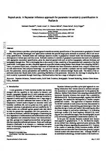
The twiddles symbol (~ ) means “is distributed as.” Because we use a uniform distribution between 0 and 1 as a prior on the rate parameter q, we write theta ~ dunif(0,1). This indicates that, a priori, each value of q is equally likely. Furthermore, k is binomially distributed with parameters q and n (i.e., k ~ dbin(theta,n)). Note that dunif and dbin are two of the predefined distributions in WinBUGS. All the distributions that are predefined in WinBUGS are listed in the distributions section in the WinBUGS manual, which can be accessed by clicking the help menu and selecting user manual (or by pressing F1). The hash symbol (#) is used for comments. The lines starting with this symbol are not executed by WinBUGS. Copy the text into an empty file and save it as “model_ rateproblemfunction.txt” in the directory from which you want to work. There are now various ways in which to proceed. One way is to work from within WinBUGS; another way is to control WinBUGS by calling it from a more general purpose program. Here, we use the statistical programming language R (R Development Core Team, 2009) to call WinBUGS, but widely used alternative research programming environments such as MATLAB are also available (Lee & Wagenmakers, 2009). A rate problem: The R script. The next step is to construct an R script to call BlackBox from R.5 When we run the script “rscript_rateproblemfunction.R,” WinBUGS starts, the MCMC sampling is conducted, WinBUGS closes, and we return to R. The object that WinBUGS has returned to R is called “rateproblem,” and this object contains all the information about the Bayesian inference for q. In particular, the “rateproblem” object contains a single sequence of consecutive draws from the posterior distribution of q, a sequence that is generally known as an MCMC chain. We use the samples from the MCMC chain to estimate the posterior distribution of q. To arrive at the posterior distribution, the samples are not plotted as a time series but as a distribution. In order to estimate the posterior distribution of q, we applied the standard density estimator in R. Figure 1 shows that the mode of the distribution is very close to .90, just as we expected. The posterior distribution is relatively spread out over the parameter space, and the 95% credible interval extends from .59 to .98, indicating the uncertainty about the value of q. Had we observed 900 wins out of a total of 1,000 games, the posterior of q would be much more concentrated around
0
.5
1.0
θ Figure 1. Posterior distribution of the rate parameter q after 9 wins out of 10 games have been observed. The dashed gray line indicates the mode of the posterior distribution at q 5 .90. The 95% credible interval extends from .59 to .98.
the mode of .90, since our knowledge about the true value of q would have greatly increased. Example 2: ObservedPlus In this section, we examine the rate problem again, but now we change the variables. Suppose we learn that before we observed the current data, 10 games had already been played, resulting in a single win. To add this information, we design a function that adds 1 to the number of observed wins, and 10 to the number of total games. So, when we use k 5 9 and n 5 10 as before, we end up with and
knew 5 kold 1 1 5 9 1 1 5 10
(2)
nnew 5 nold 1 10 5 10 1 10 5 20.
(3)
Hence, when we use our new function, the mode of the posterior distribution should no longer be .90 but .50 (10/20 5 .50). Of course, this particular problem does not require the use of WBDev and could easily be handled using plain WinBUGS code. It is the simplicity of the present problem, however, that makes it suitable as an introductory WBDev example. In order to apply WBDev to the problem above, we are going to build a function called “ObservedPlus,” using the template “VectorTemplate.odc.” This template is located in the folder “. . .\BlackBoxComponentBuilder1.5 \ WBdev \Mod.” ObservedPlus: The WBDev script. The script file “ObservedPlus.odc” shows text in three colors. The parts that are colored black should not be changed. The parts in red are comments, and these are not executed by BlackBox. The parts in blue are the most relevant parts of
Bayesian Inference Using WBDev 887 the code, because these are the parts that can be changed to create the desired function. The templates for coding the functions and distributions—written by David Lunn and Chris Jackson—come bundled with the WBDev software. These templates support the development of new functions and distributions, such that researchers can focus on the specific functions they wish to implement without having to worry about programming Component Pascal code from scratch. We now give a detailed explanation of the ObservedPlus WBDev function. The numbers (*X*) correspond to the numbers in the ObservedPlus WBDev script. For this simple example, we show some crucial parts of the WBDev scripts below. (*1*) MODULE WBDevObservedPlus;
The name of the module is typed here. We have named our module ObservedPlus. The name of the module (so the part after MODULE WBDev . . .) must start with a capital letter. (*2*) args := "ss";
Here, we must define specific arguments about the input of the function. We can choose between scalars (s) and vectors (v). A scalar means that the input is a single number. When we want to use a variable that consists of more numbers (e.g., a time series), we need a vector. This line has to correspond with the constants defined at (*3*). In our example, we use two scalars, the number of successes k and the total number of observations n. (*3*) in = 0; ik = 1;
Because of what has been defined at (*2*), WBDev already knows that there should be two variables here. We name them in and ik, with in at the first spot (with number 0) and ik at the second spot (with number 1). WBDev always starts counting at 0 and not at 1. Note that we did not name our variables n and k, but in and ik. This is because it is more insightful to use n and k later on, and it is not possible to give two or more variables the same name. Finally, note that the positions of the constants correspond to the positions of the input
of the variables into the function in the model file. We will return to this issue later. (*4*) n, k: INTEGER;
The variables that are used in the calculations need to be defined. Both variables are defined as integers, because the binomial distribution allows only integers as input: Counts of successes and the total games that are played can only be positive integers. (*5*) n k
:= SHORT(ENTIER(func.arguments[in] [0].Value())); := SHORT(ENTIER(func.arguments[ik] [0].Value())); This code takes the input values (in and ik) and gives them a name. We defined two variables in (*4*), and
we are now going to use them. What the script says here is: Take the input values in and ik and store them in the integer variables n and k. Because the input variables are not automatically assumed to be integers, we have to transform them and make sure the program recognizes them as integers. So, in other words, the first line says that n is the same as the first input variable of the function (see Figure 2), and the second line says that k is the same as the second input variable of the function. (*6*)
n:=n+10; k:=k+1; values[0] := n; values[1] := k;
This is the part of the script where we do the actual calculations. At the end of this part, we fill the output array values with the new n and k. (*7*) END WBDevObservedPlus.
Finally, we need to make sure that the name of the module at the end is the same as the name at the top of the file. The last line has to end with a period. Hence, the last line of the script is “ENDWBDevObservedPlus.” Now we need to compile the function by pressing “Ctrl1k.” Syntax errors cause WBDev to return an error message. Name this file “ObservedPlus.odc” and save it in the directory “. . .\BlackBoxComponentBuilder1.5\ WBdev\ Mod.”
Figure 2. Detailed explanation of part (*5*) of “ObservedPlus.odc.”
888 Wetzels, Lee, and Wagenmakers
model { # Uniform prior on the rate parameter theta ~ dunif(0,1) # use the function to get the new n and the new k data[1:2]