Bayesian Learning of Hierarchical Multinomial Mixture Models of ...

Bayesian Learning of Hierarchical Multinomial Mixture Models of Concepts for Automatic Image Annotation Rui Shi1, Tat-Seng Chua1, Chin-Hui Lee2, and Sheng Gao3 1

School of Computing, National University of Singapore, Singapore 117543 School of ECE, Georgia Institute of Technology, Atlanta, GA 30332, USA 3 Institute for Infocomm Research, Singapore 119613 {shirui, chuats}@comp.nus.edu.sg, [email protected], [email protected] 2

Abstract. We propose a novel Bayesian learning framework of hierarchical mixture model by incorporating prior hierarchical knowledge into concept representations of multi-level concept structures in images. Characterizing image concepts by mixture models is one of the most effective techniques in automatic image annotation (AIA) for concept-based image retrieval. However it also poses problems when large-scale models are needed to cover the wide variations in image samples. To alleviate the potential difficulties arising in estimating too many parameters with insufficient training images, we treat the mixture model parameters as random variables characterized by a joint conjugate prior density of the mixture model parameters. This facilitates a statistical combination of the likelihood function of the available training data and the prior density of the concept parameters into a well-defined posterior density whose parameters can now be estimated via a maximum a posteriori criterion. Experimental results on the Corel image dataset with a set of 371 concepts indicate that the proposed Bayesian approach achieved a maximum F1 measure of 0.169, which outperforms many state-of-the-art AIA algorithms.

1 Introduction It is said that “a picture is worth a thousand words”. Following the advances in computing and Internet technologies, the volume of digital image and video is increasing rapidly. The challenge is how to use these large and distributed image collections to increase human productivity in the reuse of valuable assets and the retrieval of information in domains such as crime prevention, medicine and publishing. Thus effective tools to automatically index images are essential in order to support applications in image retrieval. In particular, automatic image annotation has become a hot topic to facilitate content-based indexing of images. Automatic image annotation (AIA) refers to the process of automatically labeling the image contents with a predefined set of keywords or concepts representing image semantics. It is used primarily for image database management. Annotated images can be retrieved using keyword-based search, while non-annotated images can only be found using content-based image retrieval (CBIR) techniques whose performance levels are still not good enough for practical image retrieval applications. Thus AIA aims to annotate the images as accurately as possible to support keyword-based image H. Sundaram et al. (Eds.): CIVR 2006, LNCS 4071, pp. 102 – 112, 2006. © Springer-Verlag Berlin Heidelberg 2006

Bayesian Learning of Hierarchical Multinomial Mixture Models of Concepts

103

search. In this paper, we loosely use the term word and concept interchangeably to denote text annotations of images. Most approaches to AIA can be divided into two categories. The AIA models in the first category focus on finding joint probabilities of images and concepts. Cooccurrence model (CO) [12], translation model (TR) [3], and cross-media relevance model (CMRM) [7] are a few examples in this category. To represent an image, those models first segment the image into a collection of regions and quantize the visual features from image regions into a set of region clusters (so-called blobs). Given a training image corpus represented by a collection of blobs, many learning algorithms have been developed to estimate the joint probability of the concepts and blobs. In the annotation phase, the top concepts that maximize such a joint probability are assigned as concept associated with the test image. To simplify the joint density characterization, the concepts and blobs for an image are often assumed to be mutually independent [7]. As pointed out in [2], there is some contradiction with this naïve assumption because the annotation process is based on the Bayes decision rule which relies on the dependency between concepts and blobs. In the second category of approaches, each concept corresponds to a class typically characterized by a mixture model. AIA is formulated as a multi-class classification problem. In [2], the probability density function for each class was estimated by a tree structure which is a collection of mixtures organized hierarchically. Given a predefined concept hierarchy, the approach in [4] focused on finding an optimal number of mixture components for each concept class. Different from approaches in [2] and [4], ontologies are used in [14] to build a hierarchical classification model (HC) with a concept hierarchy derived from WordNet [11] to model concept dependencies. Only one mixture component was used to model each concept class. An improved estimate for each leaf concept node was obtained by “shrinking” its ML (maximum likelihood) estimate towards the ML estimates of all its ancestors tracing back from that leaf to the root. A multi-topic text categorization (TC) approach to AIA was proposed in [5] by representing an image as a high-dimension document vector with associations to a set of multiple concepts. When more mixture components are needed to cover larger variations in image samples, it often leads to poor AIA performance due to the insufficient amount of training samples and inaccurate estimation of a large number of model parameters. To tackle this problem, we incorporate prior knowledge into the hierarchical concept representation, and propose a new Bayesian learning framework called BHMMM (Bayesian Hierarchical Multinomial Mixture Model) to estimate the parameters of these concept mixture models. This facilitates a statistical combination of the likelihood function of the available training data and the prior density of the concept parameters into a well-defined posterior density whose parameters can now be estimated via a maximum a posteriori (MAP) criterion. Experimental results on the Corel image dataset with 371 concepts indicate that our proposed framework achieved an average per-concept F1 measure of 0.169 which outperforms many state-of-the-art AIA techniques. The rest of the paper is organized as follows. In Section 2 we address the key issues in general mixture models and formulate the AIA problem using hierarchical Bayesian multinomial mixture models. In Section 3 we discuss building concept hierarchies from WordNet. Two concept models, namely two-level and multi-level hierarchical models, or TL-HM and ML-HM for short, are proposed to specify the

104

R. Shi et al.

hyperparameters needed to define the prior density and perform the MAP estimation of the concept parameters. Experimental results for a 371-concept AIA task on the Corel dataset and performance comparisons are presented in Section 4. Finally we conclude our findings in Section 5.

2 Problem Formulation Since mixture models are used extensively in our study, we first describe them in detail. In [3, 7], any image can be represented by an image vector I = (n1, n2, …, nL), where L is the total number of blobs, and nl (1 l L) denotes the observed count of the lth blob in image I. Given a total of J mixture components and the ith concept ci, the observed vector I from the concept class ci is assumed to have the following probability:

≤≤ J

p ( I | Λ i ) = ∑ wi , j p( I | θi , j )

(1)

j =1

where Λi = {Wi , Θi } is the parameter set for the above mixture model, including mixJ

ture weight set Wi = {wi , j }Jj =1 ( w = 1 ), and mixture parameter set Θi = {θi , j }Jj =1 . ∑ i, j j =1

th p( I | θi, j ) is the j mixture component to characterize the class distribution. In this

paper, we use θi to denote the mixture parameters of concept class ci and θi, j to denote the parameters of the jth mixture component of the concept class ci. In this study, we assume that each mixture component is modeled by multinomial distribution as follows: L

p ( I | θi , j ) ∝ ∏ θin, lj ,l

(2)

l =1

where θi , j = (θi , j ,1 ,θi, j ,2 ,...,θi , j , L ) , θi , j ,l > 0 ,

L

∑θ l =1

i , j ,l

= 1 , and each element θi , j ,l (1

≤l≤L)

represents the probability of the lth blob occurring in the jth mixture component of the ith concept class. Now for a total of N concepts, we are given a collection of independent training images Di (Ii,t Di) for each concept class ci, the parameters in set Λi can

∈

be estimated with a maximum likelihood (ML) criterion as follows: |Di |

Λiml = arg max log p( Di | Λi ) = arg max log ∏ p( Ii,t | Λi ) Λi

Λi

(3)

t =1

We followed the EM algorithm [13] to estimate the model parameter Λi with ML criterion. In this following, we will use this model as our baseline. Although the mixture model is a simple way to combine multiple simpler distributions to form more complex ones, the major shortcoming of mixture model is that there are usually too many parameters to be estimated but not enough training images for each concept. In cases when there are larger variations among the image examples, more mixture components are needed to cover such diversities. This problem is particularly severe for natural images that tend to have large variations among them. Furthermore, for more

Bayesian Learning of Hierarchical Multinomial Mixture Models of Concepts

105

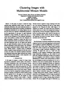
general concepts, there are likely to be larger variations among the images, too. Figure 1 shows some images from the general ‘hawaii’ concept class. It is clear a large-scale mixture model is needed to model this particular concept.

Fig. 1. Image examples from ‘hawaii’

One way to enhance the ML estimates is to incorporate prior knowledge into modeling by assuming the mixture parameters in θi , j as random variables with a joint prior density p0 (θi , j | ϕi ) with a set of parameters ϕi (often referred to as hyperparameters). The posterior probability of observing the training set can now be evaluated as: |Di |

J

p(Λi | Di ) = a ∗{∏ ∑[wi, j p( Ii,t | θi, j )]}∗ p0 (Θi | ϕi )

(4)

t =1 j =1

where a is a scaling factor that depends on Di. In contrast to conventional ML estimation shown in Eq. (3), we can impose a maximum a posterior (MAP) criterion to estimate the parameters as follows: |Di |

J

Λimap = arg max log p(Λi | Di ) = arg max log{∏ ∑[wi, j p( Ii,t | θi, j )]} ∗ p0 (Θi | ϕi ) Λi

Λi

(5)

t =1 j =1

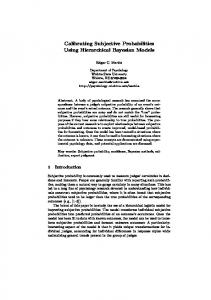
Generally speaking, the definition of the prior density p0 may come from subject matter considerations and/or from previous experiences. Due to the complexity of the data set for new applications, we often do not have enough experiences to specify the hyperparameters. However, in most practical settings, we do have prior domain knowledge which describes the dependencies among concepts often in terms of a hierarchical structure. Thus based on the posteriori density in Eq. (4), we propose a new Bayesian hierarchical multinomial mixture model (BHMMM) to characterize the hierarchical concept structure. The basic idea behind the proposed BHMMM is that the mixtures from the most dependent concepts share the same set of hyperparameters and these concept mixture models are constrained by a common prior density parameterized by this set. This is reasonable since given a concept (say, ‘leopard’) the images from its most dependent concepts (say, ‘tiger’) are often related and can be used as prior knowledge. Obviously how to define ‘most dependent’ depends on our prior domain knowledge. For example, Fig.2a shows the simplest two-level concept hierarchy in which all the concepts (c1, c2, … , cN) are derived from the root node labeled ‘entity’. The structure of this two-level hierarchical model (TL-HM) is shown in Fig.2b, in which all the mixture parameters share only one common prior density with the same hyperparameter set ϕ0 . The advantage of using such a two-level concept hierarchy is that we don’t need any prior domain knowledge. However, the two-level concept hierarchy can not capture all the concept dependencies accurately. For instance, there is not much

106

R. Shi et al. ϕ0 …

‘entity’

θ1,1 θ1,2 ,..., θ1, J … θN,1 , θN,2 ,..., θN,J

… ‘c1’

…

‘c2’

‘cN’

D1

(a) Two-level concept hierarchy

(b) Two-level Hierarchical Model (TL-HM) ϕi

‘ci’

…

θ i ,1 θ i ,2 ,..., θ i , J

… ‘ci,1’

‘ci,2’

DN

… ‘ci,M’

Di

(c) Sub-tree of multi-level concept hierarchy

(d) Multi-level HM (ML-HM)

Fig. 2. An illustration of the proposed BHMMM

dependency between the concepts of ‘buildings’, ‘street’ and the concept of ‘tiger’. To better model the concept dependencies, we first derive a concept hierarchy through WordNet in Section 3.1. Fig. 2c shows a sub-tree of multi-level concept hierarchy in which the concepts (ci,1, ci,2, … , ci,M) are derived from their parent node labeled ‘ci’. We then extend the two-level to multi-level hierarchical model (ML-HM) by characterizing the prior density parameters for the ith concept mixture model with a separate set of hyperparameters ϕi , as shown in Fig 2d. Then the mixtures from concepts ci,1, ci,2, … , ci,M share the same set of hyperparameters ϕi . Clearly more hyperparameters are needed in ML-HM than in TL-HM. We will compare the two models in Section 3.

3 Hierarchical Models 3.1 Building Concept Hierarchy As discussed in Section 2, we are interested in accurately model the concept dependencies which requires finding relationships between concepts. Ontologies, such as the WordNet [11], are convenient specifications of such relationships. WordNet is an electronic thesaurus to organize the meaning of English nouns, verbs, adjectives and adverbs into synonym sets, and are used extensively in lexical semantics acquisition [9]. Every word in WordNet has one or more senses, each of which has a distinct set of related words through other relations such as hypernyms, hyponyms or holonyms. For example, the word ‘path’ is a concept in our corpus. ‘Path’ has four senses in WordNet and each sense is characterized by a sequence of words (hypernyms): (a) path course action activity abstract entity; (b) path way artifact object entity; (c) path, route line location object entity, and (d) path, track line location object entity. Thus the key for building a concept hierarchy is to disambiguate the senses of words. Since the words used as annotations in our data set (Corel CD) are nouns, we only use the ‘hypernym’ relation which points to a word that is more generic than a given

←

←

←

← ← ←

← ←

←

← ←

←

← ← ←

←

←

Bayesian Learning of Hierarchical Multinomial Mixture Models of Concepts

107

word in order to disambiguate the sense of words. We further assume that one word corresponds to only one sense in the whole corpus. This is reasonable as a word naturally has only one meaning within a context. With this assumption, we adopt the basic idea that the sense of a word is chosen if the hypernyms that characterize this sense are shared by its co-occurred words in our data set. For example, the co-occurred words of ‘path’ are ’tree’, ’mountain’, ‘wall’, ‘flower’ and so on. Thus path way artifact object entity is chosen since this sense is mostly shared by these co-occurred words of ‘path’. Our approach for disambiguating the senses of words is similar to that used in [1]. After this step of word sense disambiguation, every word is assigned a unique sense characterized by its hypernyms. Thus, we can easily build a multi-level concept hierarchy with ‘entity’ as the root node of the overall concept hierarchy.

← ←

←

←

3.2 Definition of Prior Density Based on the MAP formulation in Eq. (5), three key issues need to be addressed: (i) choosing the form of the prior density, (ii) specification of the hyperparameters, and (iii) MAP estimation. It is well-known that a Dirichlet density is the conjugate prior for estimating the parameters of multinomial distributions so that the posterior distribution has a similar form to the Dirichlet density, which makes it easy to estimate its parameters. Such methods have been used successfully in automatic speech recognition for adaptive estimation of histograms, mixture gains, and Markov chains [6, 9]. We adopt Dirichlet distribution as the prior distribution p0 with hyperparameter ϕ (as in Figures 2b and 2d), as follows: Γ(∑ l =1ϕ0,l ) L

p0 (θi , j | ϕ0 ) =

∏

L l =1

Γ(ϕ0,l )

L

l =1

L (ϕ −1) or p (θ | ϕ ) = Γ( ∑ l =1ϕi ,l ) θi , ji,l,l ∏ 0 i, j i L Γ ϕ 1 l = ( ) ∏ l =1 i,l L

∏ θ i , j ,l

(ϕ0,l −1)

(6)

≤≤

where ϕi = (ϕi ,1 , ϕi ,2 ,..., ϕi , L ) , ϕi ,l > 0 ,1 l L, and the hyperparameter ϕi ,l can be interpreted as ‘prior observation counts’ for the lth blob occurring in the ith concept class, and Γ( x) is the Gamma function. As discussed in Section 2, the performances of the proposed BHMMM framework depend on the structure of the concept hierarchy. This is related to how we intend to specify the hyperparameters. The remaining issue is the estimation of hyperparameters which will be addressed next. 3.3 Specifying Hyperparameters Based on Concept Hierarchy We first discuss how to specify hyperparameters based on two-level concept hierarchy as shown in Figures 2a and 2b. If we assume that all mixture parameters θi, j share the same set of hyperparameters, ϕ0 , we can then adopt an empirical Bayes approach [6] to estimate these hyperparameters. Let Θ0 = {θ1ml ,θ2ml ,...,θ Nml } denote the mixture parameter set estimated with ML criterion as in Eq. (3). We then pretend to view Θ0 as a set of random samples from the Dirichlet prior p0 (ϕ0 ) in Eq. (6). Thus the ML estimate of ϕ0 maximizes the logarithm of the likelihood function, log p0 (Θ0 | ϕ0 ) . As

108

R. Shi et al.

pointed out in [10], there exists no closed-form solution to this ML estimate, and the fixed-point iterative approach [10] can be adopted to solve for the ML estimate based on a preliminary estimate of ϕ0old that satisfies the following: L

old Ψ(ϕ0,new l ) = Ψ(∑ϕ0,l ) + l =1

1 N J ∑∑ logθi,mlj,l N × J i =1 j =1

(7)

where Ψ( x) = d Γ( x) is known as the digamma function. More details can be found dx

in [10]. For characterizing multi-level concept hierarchy, we assume that all mixture parameters θi, j in the ith concept share the same set of hyperparameters, ϕi , then we can use the data in Di to obtain a preliminary ML estimate θi and pretend to view θi as a set of random samples from the Dirichlet prior p0 (ϕi ) in Eq. (6). Then the ML estimate of ϕi can be solved by maximizing the log-likelihood log p0 (θi | ϕi ) . The above fixed-point iterative approach [10] can again be adopted to solve for the ML estimate based on a preliminary estimate of ϕiold that satisfies the following: L

old Ψ(ϕinew ,l ) = Ψ(∑ϕi ,l ) + l =1

1 J ∑ logθi,mlj ,l J j =1

(8)

It is clear that the concept-specific hyperparameter estimate ϕi uses less data in Eq. (8) than those in Eq. (7) for general hyperparameter estimate ϕ0 . 3.4 MAP Estimation of Mixture Model Parameters With the prior density given in Eq. (6) and the hyperparameters specified in Eq. (7) or (8), we are now ready to solve MAP estimation in Eq. (5) as follows: By traversing the nodes one by one from left to right in the same level, and from root level down to the leaf level, for each node ci in the concept hierarchy: ♦ Let cip denote the parent node of ci and p0 (ϕipml ) denote the prior density function for the mixture model parameters of cip, we have: |Di |

J

t =1

j =1

Λimap = argmax log p(Λi | Di ) = argmaxlog{∏[∑[wi, j p(Ii,t | θi, j )]}∗ p0 (Θi | ϕipml ) Λi

Λi

where ϕipml = (ϕipml,1 , ϕipml,2 ,..., ϕipml, L ) , ϕipml,l > 0 ,1

(9)

≤l≤L.

♦ If ci has the child node, then the prior density function p0 (ϕi ) for mixture parameters of ci can be calculated by the approach described in Section 4.

ϕiml = arg max log ∏ j p0 (θi,mlj | ϕi ) ϕi

We simply extend the EM algorithm in [13] to solve Eq. (9). Given a preliminary estimate of Λinew , the EM algorithm can be described as follows:

Bayesian Learning of Hierarchical Multinomial Mixture Models of Concepts new new E-step: wiold , θiold , , j = wi , j , j = θi , j

J old J , Λiold = {{wiold , j } j =1 ,{θi , j } j =1}

L

p ( j | I i ,t , Λ iold ) =

p ( I i ,t | θ J

∑ p( I j =1

| Di |

M-step: wnew = i, j

∑ p( j | I t =1

i ,t

i ,t

, Λ iold )

109

old i, j

) p0 (θ

old i, j

| ϕ )w ml ip

old i, j

old ml old | θ iold , j ) p0 (θ i , j | ϕ ip ) wi , j

| Di |

,

θ

| Di |

new i , j ,l

=

∑ p( j | I

t =1 | Di | L

i ,t

∑∑ p( j | I t =1 l =1

=

old wiold , j ∏ (θ i , j ,l )

ni ,t ,l +ϕipml,l −1

.

l =1

J

L

∑ w ∏ (θ j =1

old i, j

l =1

old i , j ,l

)

ni ,t ,l +ϕipml,l −1

, Λ iold ) × ( ni ,t ,l + ϕipml,l − 1) i ,t

.

, Λ iold ) × ( ni ,t ,l + ϕipml,l − 1)

≤≤

Here |Di| denotes the size of training set Di for ci, ni,t,l (1 l L) denotes the observed count of the lth blob in the image Ii,t Di, and p( j | I i,t , Λiold ) is the probability that the

∈

jth mixture component fits the image Ii,t, given the parameter Λiold .

4 Testing Setup and Experimental Results Following [3, 7], we conduct our experiments on the same Corel CD data set, consisting of 4500 images for training and 500 images for testing. The total number of region clusters (blobs) is L=500. In this corpus, there are 371 concepts in the training set but only 263 such concepts appear in the testing set, with each image assigned 1-5 concepts. After the derivation of concept hierarchy as discussed in Section 3.1, we obtained a concept hierarchy containing a total of 513 concepts, including 322 leaf concepts and 191 non-leaf concepts. The average number of children of non-leaf concepts is about 3. If a non-leaf concept node in the concept hierarchy doesn’t belong to the concept set in Corel CD corpus, then its training set will consist of all the images from its child nodes. As with the previous studies on this AIA task, the AIA performance is evaluated by comparing the generated annotations with the actual image annotations in the test set. We assign a set of five top concepts to each test image based on their likelihoods. Table 1. Performances of our approaches Models Baseline Baseline TL-HM TL-HM ML-HM (mixture number) (J=5) (J=25) (J=5) (J=25) (J=5) # of concepts (recall>0) 104 101 107 110 117 Mean Per-concept metrics on all 263 concepts on the Corel dataset Mean Precision

0.102

0.095

0.114

ML-HM (J=25) 122

0.121

0.137

0.142

Mean Recall

0.168

0.159

0.185

0.192

0.209

0.225

Mean F1

0.117

0.109

0.133

0.140

0.160

0.169

We first compare the performances of TL-HM and ML-HM with the baseline mixture model. In order to highlight the ability to cover large variations in the image set, we select two different numbers of mixtures (5 and 25) to emulate image variations.

110

R. Shi et al.

These two numbers are obtained by our empirical experiences. The results in terms of averaging precision, recall and F1 are tabulated in Table 1. From Table 1, we can draw the following observations: (a) The performance of baseline (J=25) is worse than that of baseline (J=5). This is because the number of training image examples are same in both cases and we are able to estimate the small number of parameters for baseline (J=5) more accurately. This result highlights the limitation of mixture model when there are large variations in image samples. (b) The F1 performances of TL-HM and ML-HM are better than that of the baseline (J=5). This indicates that the proper use of prior information is important to our AIA mixture model. (c) Compared with TL-HM (J=5, 25), ML-HM (J=5, 25) achieves about 20% and 21% improvements on F1 measure. This shows that the use of concept hierarchy in ML-HM results in more accurate estimate of prior density, since ML-HM permits a concept node to only inherit the prior information from its parent node. Overall, ML-HM achieves the best performance of 0.169 in terms of F1 measure. Table 2. Performances of state-of-the-art AIA models Models #concepts with recall>0

CO [8,12] 19

TR [3,8] 49

CMRM [7,8] 66

HC [14] 93

Mean per-concept results on all 263 concepts on the Corel dataset Mean Per-concept Precision

0.020

0.040

0.090

0.100

Mean Per-concept Recall

0.030

0.060

0.100

0.176

For further comparison, we tabulate the performances of a few representative stateof-the-art AIA models in Table 2. These are all discrete models which used the same experimental settings as in Table 1. From Table 2, we can draw the following observations: (a) Among these models, HC achieved the best performance in terms of precision and recall measures, since HC also incorporated the concept hierarchy derived from the WordNet into the classification. This further reinforces the importance of utilizing the hierarchical knowledge for AIA task. (b) Compared with HC which used only one mixture for each concept class and adopted ML criterion to estimate the parameters, HM-ML (J=25) achieved about 40% and 28% improvements on the measure of mean per-concept precision and mean per-concept recall respectively. This demonstrates again that HM-ML is an effective strategy to AIA task. To analyze the benefits of our strategies, we perform a second test by dividing the testing concepts into two sets – designated as primitive concept (PC) and Table 3. Performances of our approaches in PC and NPC Models Baseline TL-HM ML-HM Baseline TL-HM ML-HM (mixture components) (J=5) (J=25) (J=25) (J=5) (J=25) (J=25) Concept Split Results with 137 concepts in PC Results with 126 concepts in NPC #concepts (recall>0) Mean Per-concept F1

44 0.099

45 0.116

49 0.141

60 0.133

65 0.162

73 0.196

Bayesian Learning of Hierarchical Multinomial Mixture Models of Concepts

111

non-primitive concept (NPC) sets. The PC concepts, such as ‘tiger’, ‘giraffe’ and ‘pyramid’, have relatively concrete visual forms. On the other hand the NPC concepts, such as ‘landscape’, ‘ceremony’ and ‘city’, do not exhibit concrete visual descriptions. The total number of concepts is 137 and 126 for NPC and PC sets respectively. We expect the use of ML-HM that utilizes the concept hierarchy to be more beneficial to the concepts in the NPC set than those in the PC set. In this test, we select the best performing system in each category, namely Baseline (J=5), TL-HM (J=25) and ML-HM (J=25). The results on the PC and NPC sets are presented in Table 3 for the F1 measure. It is clear that ML-HM (J=25) achieves the best performance on the NPC set among the three cases. ML-HM can detect 13 more concepts on the NPC set as compared to the baseline but only 5 more concepts on the PC set. In terms of the F1 measure, ML-HM achieves about 47% and 42% improvement over the baseline on the NPC and PC sets respectively. Overall, both ML-HM and TL-HM outperform the Baseline on both the PC and NPC sets. The ML-HM model, being able to take full advantage of the multi-level concept structure to model the concepts in the NPC set, performs better than TL-HM model. Table 4. Mean number of training examples

Concept Split Number of concept classes in each group Mean number of training examples for each concept class

(1) NPC #concepts (recall>0) 77

(2) NPC #concepts (recall=0) 49

(3) PC #concepts (recall>0) 54

(4) PC #concepts (recall=0) 83

103.34

19.25

98.11

12.35

To analyze the effect of the number of training examples on the performances, we further analyze the results by splitting the testing concepts into four groups, two concept groups for NPC with recall>0 and recall=0, and two concept groups for PC with recall>0 and recall=0. In arriving at the number of concept classes of 77 (or 54) for NPC (or PC), we simply combine all the classes with recall>0 obtained from the three methods (Baseline TL-HM and ML-HM). From the results presented in Table 4, the mean number of training examples from (1) and (3) is significantly more than that in (2) and (4). Although we didn’t investigate the qualitative relationships between the number of training examples and the performances, this result clearly states that if the number of training examples is too small, our proposed BHMMM could not achieve good performances. So from this perspective, how to acquire more training examples for concept classes is an important problem which we will tackle in our future work.

5 Conclusion In this paper, we incorporated prior knowledge into hierarchical representation of concepts to facilitate modeling of multi-level concept structures. To alleviate the potential difficulties arising in estimating too many parameters with insufficient training images, we proposed a Bayesian hierarchical mixture model framework. By

112

R. Shi et al.

treating the mixture model parameters as random variables characterized by a joint conjugate prior density, it facilitates a statistical combination of the likelihood function of the available training data and the prior density of the concept parameters into a well-defined posterior density whose parameters can now be estimated via a maximum a posteriori criterion. On the one hand when no training data are used, MAP estimate is the mode of the prior density. On the other hand when a large of amount of training data is available the MAP estimate can be shown to asymptotically converge to the conventional maximum likelihood estimate. This desirable property makes the MAP estimate an ideal candidate for estimating a large number of unknown parameters in large-scale mixture models. Experimental results on the Corel image dataset show that the proposed BHMMM approach, using a multi-level structure of 371 concept with a maximum of 25 mixture components per concept, achieves a mean F1 measure of 0.169, which outperforms many state-of-the-art techniques for automatic image annotation.

References [1] K. Barnard, P. Duygulu and D. Forsyth, “Clustering Art”, In Proceedings of CVPR, 2001. [2] G. Carneiro and N. Vasconcelos, “Formulating Semantic Image Annotation as a Supervised Learning Problem”, In Proceedings of CVPR, 2005. [3] P. Duyulu, K. Barnard, N. de Freitas, and D. Forsyth, “Object Recognition as Machine Translation: Learning a Lexicon for a Fixed Image Vocabulary”, In Proc. of ECCV, 2002. [4] J. P. Fan, H. Z. Luo and Y. L. Gao, “Learning the Semantics of Images by Using Unlabeled Samples”, In Proceedings of CVPR, 2005. [5] S. Gao, D.-H. Wang and C.-H. Lee, “Automatic Image Annotation through Multi-Topic Text Categorization”, In Proceedings of. ICASSP, Toulouse, France, May 2006. [6] Q. Huo, C. Chan and C.-H. Lee, “Bayesian Adaptive Learning of the Parameters of Hidden Markov Model for Speech Recognition”, IEEE Trans. Speech Audio Processing, vol. 3, pp. 334-345, Sept. 1995. [7] J. Jeon, V. Lavrenko, and R. Manmatha, “Automatic Image Annotation and Retrieval Using Cross-Media Relevance Models”, In Proceedings of the 26th ACM SIGIR, 2003. [8] V. Lavrenko, R. Manmatha and J. Jeon, “A Model for Learning the Semantics of Pictures”, In Proceedings of the 16th Conference on NIPS, 2003. [9] C.-H. Lee and Q. Huo, “On Adaptive Decision Rules and Decision Parameter Adaptation for Automatic Speech Recognition”, In Proceedings of the IEEE, vol. 88, no. 8, Aug, 2000. [10] T. Minka, http://www.stat.cmu.edu/~minka/papers/dirichlet, “Estimating a Dirichlet Distribution”, 2003. [11] G. A. Miller, R. Beckwith, C. Fellbaum, D. Gross and K. J. Miller, “Introduction to WordNet: an on-line lexical database”, Intl. Jour. of Lexicography, vol. 3, pp. 235-244, 1990. [12] Y. Mori, H. Takahashi, and R. Oka, “Image-to-Word Transformation Based on Dividing and Vector Quantizing Images with Words”, In Proceedings of MISRM, 1999. [13] J. Novovicova and A. Malik, “Application of Multinomial Mixture Model to Text Classification”, Pattern Recognition and Image Analysis, LNCS 2652, pp. 646-653, 2003. [14] M. Srikanth, J. Varner, M. Bowden and D. Moldovan, “Exploiting Ontologies for Automatic Image Annotation”, In Proceedings of the 28th ACM SIGIR, 2005.