Bayesian Regression. Given that β is the ... computations follow the classification
case: Where the ... What these results show is that Bayesian regression can be ...
Nonlinear Regression: – X. N .... Memory-Based linear-interpolation method.
Bayesian Linear Regression • Bayesian treatment: avoids the over-fit and leads to an automatic way of determining the model complexity using only the training data. • We start by defining a simple likelihood conjugate prior, • For example, a zero-mean Gaussian prior governed by a precision parameter:
This prior, when combines with the “least squares” likelihood via Bayes rule, yields the posterior distribution:
r p(w | t , X) = N ( w;mN ,SN )
For example, we will show that for the prior above, and for a matrix of transformed predictors Φ -1
r w = " (# # + $I) # t T
!
CSCI 5521: Paul Schrater
In other words:
%1
T
cov[w] = (#T # + $I)
RECALL-Probabilistic interpretation
0
Likelihood
CSCI 5521: Paul Schrater
0
20
CSCI 5521: Paul Schrater
Bayesian Linear Regression • Given target values, modeled as a sum of basis functions plus Gaussian noise
• Then the likelihood is Gaussian
• Assuming a Gaussian prior makes the posterior tractable
CSCI 5521: Paul Schrater
Bayesian Regression • The posterior is straightforward to derive. The computations follow the classification case: r p(w | t , X, " ) = N(w | µN ,SN ) r # p( t | w, X, " ) p(w) r T = N ( t | w $, " %1I)N (w | µ0 ,S0 )
! the posterior mean and variance are given by: Where
Given that β is the noise in the measurements CSCI 5521: Paul Schrater
Basic Results for Gaussians • The results stem from the fact that multiplying two Gaussians is Gaussian (although no longer normalized). In particular,
CSCI 5521: Paul Schrater
Special Cases • Prior on w
• Ridge Regression Posterior on w
CSCI 5521: Paul Schrater
From Ridge to Lasso etc • A family of priors for regularized regression:
CSCI 5521: Paul Schrater
Visualizing Bayesian Regression 3
1
2
4
Sequential Bayesian Learning: As each data point comes in,the posterior on w is updated. Lines show samples from the posterior distribution. 1 No Data 2 One data point 3 Two data points 4 Twenty data points CSCI 5521: Paul Schrater
Predictive Distribution • To predict new datapoints, we need to marginalize the basic regression model across our uncertainty in the regression coefficients (model averaging
(
p y pred
r t ," , # =
) $ p( y
pred
$ N (y = $ N (y = N (y =
r w, # ) p(w | t , X,", # )dw
pred
r | %w, # I)N w | S ( S µ + #% t ),SN dw
pred
| %w, # &1I)N ( w | mN ,SN ) dw
&1
pred
(
&1 N
| %mN , # &1I + %SN %T )
T
&1 0 0
)
where SN = S0"1 + #$T $
CSCI 5521: Paul Schrater
!
More Results
CSCI 5521: Paul Schrater
Predictive Distribution
CSCI 5521: Paul Schrater
Bayes does model averaging: with the average across set of w Samples from the Posterior Distribution on w
CSCI 5521: Paul Schrater
Posterior mean on w and the equivalent kernel
CSCI 5521: Paul Schrater
Another Meaning for the Kernel • In the Bayesian framework, it is easy to show that the equivalent kernel is the covariance matrix of the predictive distribution.
What these results show is that Bayesian regression can be Viewed as a kernel based algorithm. Rather than choosing the Weights on a fixed set of kernels (SVR), the kernels are constructed from the data modeling assumptions. CSCI 5521: Paul Schrater
Gaussian Processes in Machine Learning
CSCI 5521: Paul Schrater
Outline of the talk • Gaussian Processes (GP) [ma05, rs03] – Bayesian Inference – GP for regression – Optimizing the hyperparameters
• Applications – GP Latent Variable Models [la04] – GP Dynamical Models [wa05]
CSCI 5521: Paul Schrater
GP: Introduction • Gaussian Processes: – Definition: A GP is a collection of random variables, any finite number of which have joint Gaussian Distribution • Distribution over functions: –
• Gaussian Distribution: over vectors –
• Nonlinear Regression: – XN – tN
… Data Points … Target Vector
• Infer Nonlinear parameterized function, y(x;w), predict values tN+1 for new data points xN+1 • E.g. Fixed Basis Functions – CSCI 5521: Paul Schrater
Bayesian Inference of the parameters
• Posterior propability of the parameters: –
y(x;w)
Probability that the observed data points have been generated by
• Often separable Gaussian distribution is used
–
– Each data point ti differing from y(xi;w) by additive noise
priors on the weights
• Prediction is made by marginalizing over the parameters – – Integral is hard to calculate • Sample parameters w from the distribution chain Monte Carlo techniques • Or Approximate with a Gaussian Distribution
CSCI 5521: Paul Schrater
with Markov
Bayesian Inference: Simple Example
• •
GP: is a Gaussian distribution Example: H Fixed Basis functions, N input points – – –
Prior on w: Calculate prior for y(x) :
•
Prior for the target values –
• • CSCI 5521: Paul Schrater
generated from y(x;w) + noise:
Covariance Matrix: Covariance Function
k ( xi , x j ) = ! w2#h ( xi )#h ( x j ) + " ij! v2
Predicting Data • Infer tN+1 given tN : – Simple, because conditional distribution is also a Gaussian – – Use incremental form of
k T = [k ( xN +1 , x1 ),..., k ( xN +1 , xN )] ! = k ( x N +1 , x N +1 )
CSCI 5521: Paul Schrater
Predicting Data
•
We can rewrite this equation –
Use partitioned inverse equations to get from
–
2 ˆ P(tn +1 | t N ) = Normal (t N +1 , ! tˆN +1 )
– –
Predictive mean: •
–
CSCI 5521: Paul Schrater
Usually used for the interpolation
Uncertainty in the result :
Bayesian Inference: Simple Example
• How does the covariance matrix look like? – – – Usually N >> H: Q has not full rank, but C has (due to the addition of I) – Simple Example: 10 RBF functions, uniformly distributed over the input space
CSCI 5521: Paul Schrater
Bayesian Inference: Simple Example •
Assume uniformly spaced basis functions,
•
Solution of the integral – Limits of integration to
– More general form
~ k ( xn , xm ) = k ( xn , xm ) =
CSCI 5521: Paul Schrater
Gaussian Processes
– – CSCI 5521: Paul Schrater
Only CN needs to be inverted (O(N³)) Prediction depend entirely on C and the known targets tN
Gaussian Processes: Covariance functions • Must generate a non-negative definite covariance matrix for any set of points – {", ! } –
•
Hyperparameters of C
Some Examples: – RBF: – Linear:
•
Some Rules: – Sum: – Product: – Product Spaces:
~ k ( xn , xm ; ") = k ( xn , xm ; ") + $ nm # !1 ~ k ( xn , xm ) = ~ k ( xn , xm ) = " # xnT xm + !
,
~ ~ ~ k ( xn , xm ) = k 2 ( xn , xm ) + k1 ( xn , xm ) ~ ~ ~ k ( xn , xm ) = k 2 ( xn , xm ) ! k1 ( xn , xm ) ~ ~ ~ k ( z n , z m ) = k 2 ( xn , xm ) + k1 ( yn , ym )
CSCI 5521: Paul Schrater
Adaption of the GP models
•
$ = {# , " , ! }
Hyperparameters: –
Typically : •
=>
• •
Log marginal Likelihood (first term) – – –
Optimize via gradient descent (LM algorithm) First term: complexity penalty term •
–
•
=> Occams Razor ! Simple models are prefered
Second term: Data-fit measure
Priors on hyperparameters (second term) – –
Typically used:P ($) = Prefer small parameters: • • •
– CSCI 5521: Paul Schrater
! P(% )#!%
Small output scale ( ) ! Large width for the RBF ( ) Large noise variance ( ) !
i
!
Additional mechanism to avoid overfitting
"1 i
GP: Conclusion/Summary • • • •
Memory-Based linear-interpolation method y(x) is uniquely defined by the definition of the C-function Also Hyperparameters are optimized Defined just for one output variable – Individual GP for each output variable – Use the same Hyperparameters
•
Avoids overfitting – Tries to use simple models – We can also define priors
• • •
No Methods for input data selection Difficult for a large input data set (Matrix inversion O(N³)) – CN can also be approximated, up to a few thousand input points possible
Interpolation : No global generalization possible
CSCI 5521: Paul Schrater
Applications of GP •
Gaussian Process Latent Variable Models (GPLVM) [la04] – –
•
Style Based Inverse Kinematics [gr04] Gaussian Process Dynamic Model (GPDM) [wa05]
Other applications: – –
GP in Reinforcement Learning [ra04] GP Model Based Predictive Control [ko04]
CSCI 5521: Paul Schrater
Propabilistic PCA: Short Overview
•
Latent Variable Model: –
•
Project high dimensional data (Y, d-dimensional) onto a low dimensional latent space (X, q-dimensional, q O(N³)
CSCI 5521: Paul Schrater
GPLVM: illustrative Result •
Oil data set – 3 classes coresponding to the phase flow in a pipeline: stratified, annular, homogenous – 12 input dimensions
PCA CSCI 5521: Paul Schrater
GPLVM
Style based Inverse Kinematics
•
Use GPLVM to represent Human motion data – Pose: 42-D vector q (joints, position, orientation) – Always use one specific motion style (e.g. walking) – Feature Vectors: y • • • •
Joint Angles Vertical Orientation Velocity and Acceleration for each feature > 100 dimensions
– Latent Space: usually 2-D or 3-D
•
Scaled Version of GPLVM – Minimize negative log-posterior likelihood
CSCI 5521: Paul Schrater
Style-based Inverse Kinematics •
Generating new Poses (Predicting) : – –
We do not know the location in latent space Negative Log Likelihood for a new pose (x,y)
•
Standard GP equations:
–
•
•
Variance indicates uncertainty in the prediction » Certainty is greatest near the training data
=> keep y close to prediction f(x) while keep x close to the training data
Synthesis: Optimize q given some constraints C –
Specified by the user, e.g. positions of the hands, feets
CSCI 5521: Paul Schrater
SBIK: Results •
Different Styles: –
Base-Ball Pitch
–
Start running
CSCI 5521: Paul Schrater
SBIK: Results •
Posing characters – Specify position in 2-D latent space
•
Specify/Change trajectories
CSCI 5521: Paul Schrater
GP Dynamic Model [wa05] •
SBIK does not consider the dynamics of the poses (sequential order of the poses) –
•
Model the dynamics in latent Space X
2 Mappings: – –
Dynamics in Low dimensional latent space X (q dimensional), markov property Mapping from latent space to data space Y (d dimensional) (GPLVM)
–
Model both mappings with GP
CSCI 5521: Paul Schrater
GPDM: Learn Mappings • Fit parameters: Weights, number of basis functions + shape – difficult
• From GP view: parameters should be marginalized out
CSCI 5521: Paul Schrater
GPDM: Learn Mapping g •
Learning Mapping g: –
•
Mapping from latent space X to high dimensional output space Y
Prior on Y
– –
Independent Gaussian for every output dimension W = diag(w1,..,wD) … scaling matrix, to account for different variances in different data dimensions
•
RBF Covariance Function
•
Hyperparameters:
CSCI 5521: Paul Schrater
GPDM: Learn dynamic Mapping f •
Mapping g: – Mapping from latent space X to high dimensional output space Y – Same as in Style based kinematics
•
GP: marginalizing over weights A –
•
Markov property –
•
Again multivariate GP: Posterior distribution on X
CSCI 5521: Paul Schrater
GPDM: Learn dynamic Mapping f
T
•
X = [ x ,..., xN ]
Priorsoutfor X: 2 –
• Future xn+1 is target of the approximation
– x1 is assumed to have Gaussian prior – KX …(N-1)x(N-1) kernel matrix
– Joint distribution of the latent Variables is not Gaussian • xt does occur outside the covariance matrix
CSCI 5521: Paul Schrater
GPDM: Algorithm •
Minimize negative log-posterior –
– Minimize with respect to – Data: • • • • •
and
56 Euler angles for joints 3 global (torso) pose angles 3 global (torso) translational velocities Mean-subtracted X was initialized with PCA coordinates
– Numerical Minimization through Scaled Conjugate Gradient
CSCI 5521: Paul Schrater
GPDM: Results
• • •
(b) Style-based Inverse Kinematics (a) GPDM Smoother trajectory in latent space!
CSCI 5521: Paul Schrater
GPDM: Visualization
• •
(a) Latent Coordinates during 3 walk cycles (c) 25 samples from the distribution –
•
Sampled with the hybrid Monte Carlo Method
(d) Confidence with which the model reconstructs the pose from the latent position –
High probability tube around the data
CSCI 5521: Paul Schrater
GPDM: Online generation of new motion •
Mean Prediction Sequences – Standard GP equations
– Always take the predicted mean point – The same for new poses ( ) – Long sequences generated by mean prediction can diverge from the data
•
Optimization – Prevent the Mean Prediction from drifting away from training data – Optimize the likelihood of the new sequence – is lower near the training data, consequently the likelihood of xt+1 can be increased by moving xt closer to the training data – Optimization process is initialized with mean prediction sequence
CSCI 5521: Paul Schrater
GPDM: Mean Prediction and Optimization
(a)
(b)
• (a) Mean prediction • (b) Optimization CSCI 5521: Paul Schrater
Summary/Conclusion • GPLVM – GPs are used to model high dimensional data in a low dimensional latent space – Extension of the linear PCA formulation
• Human Motion – Generalizes well from small datasets – Can be used to generate new motion sequences – Very flexible and naturally looking solutions
• GPDM – additionally learn the dynamics in latent space
CSCI 5521: Paul Schrater
Literature • • • • • • • •
[ma05] D. MacKay, Introduction to Gaussian Processes, 2005 [ra03] C. Rasmussen, Gaussian Processes in Machine Learning, 2003 [wa05] J. Wang and A. Hertzmann, Gaussian Process Dynamical Models, 2005 [la04] N. Lawrence, Gaussian Process Latent Variable Models for Visualisation of High Dimensional Data, 2004 [gr04] K. Grochow, Z. Popovic, Style-Based Inverse Kinematics, 2004 [ra04] C. Rasmussen and M. Kuss, Gaussian Processes in Reinforcement Learning, 2004 [ko04] J. Kocijan, C. Rasmussen and A. Girard, Gaussian Process Model Based Predictive Control, 2004 [sh04] J. Shi, D. Titterington, Hierarchical Gaussian process mixtures for regression
CSCI 5521: Paul Schrater