Bayesian Maximum Entropy (Two-Dimensional ...

Bayesian Maximum Entropy (Two-Dimensional) Lifetime Distribution Reconstruction from Time-Resolved Spectroscopic Data ´ RENZ-FONFRIÁ* and HIDEKI KANDORI VICTOR A. LO Department of Materials Science and Engineering, Nagoya Institute of Technology, Showa-ku, Nagoya 466-8555, Japan

Time-resolved spectroscopy is often used to monitor the relaxation processes (or reactions) of physical, chemical, and biochemical systems after some fast physical or chemical perturbation. Time-resolved spectra contain information about the relaxation kinetics, in the form of macroscopic time constants of decay and their decay associated spectra. In the present paper we show how the Bayesian maximum entropy inversion of the Laplace transform (MaxEnt-iLT) can provide a lifetime distribution without sign-restrictions (or two-dimensional (2D)-lifetime distribution), representing the most probable inference given the data. From the reconstructed (2D) lifetime distribution it is possible to obtain the number of exponentials decays, macroscopic rate constants, and exponential amplitudes (or their decay associated spectra) present in the data. More importantly, the obtained (2D) lifetime distribution is obtained free from pre-conditioned ideas about the number of exponential decays present in the data. In contrast to the standard regularized maximum entropy method, the Bayesian MaxEnt approach automatically estimates the regularization parameter, providing an unsupervised and more objective analysis. We also show that the regularization parameter can be automatically determined by the L-curve and generalized crossvalidation methods, providing (2D) lifetime reconstructions relatively close to the Bayesian best inference. Finally, we propose the use of MaxEnt-iLT for a more objective discrimination between data-supported and data-unsupported quantitative kinetic models, which takes both the data and the analysis limitations into account. All these aspects are illustrated with realistic time-resolved Fourier transform infrared (FT-IR) synthetic spectra of the bacteriorhodopsin photocycle. Index Headings: Exponential analysis; Time-resolved spectroscopy; Maximum entropy; Bayesian inference; Inverse problems; Lifetime distribution; Bacteriorhodopsin.

INTRODUCTION Time-resolved spectroscopy is often used to monitor the relaxation processes of physical, chemical, and biochemical systems after some physical or chemical perturbation (e.g., temperature jump, photoreaction, etc). Relevant examples in the literature include protein folding/unfolding, ligand biding/ release, and photoreactions.1–3 The final goal is to obtain the relaxation mechanism (number of intermediate states and their interconversion rate constants) and the spectroscopic properties of the kinetic intermediates.4 When the relaxation of the system to the equilibrium is governed by linear differential equations, the relative fraction of intermediates as a function of time will be generally given by as many exponential decays as kinetic intermediates are present,5 or even by a distribution of exponentials.6–8 Both the exponential amplitudes and macroscopic rate constants will be non-trivially related (except in the most simple cases) to the intrinsic rate constants involved in the relaxation pathway.9,10 Received 10 October 2006; accepted 19 January 2007. * Author to whom correspondence should be sent. E-mail: victor.lorenz@ gmail.com.

428

Volume 61, Number 4, 2007

From the time-resolved spectroscopic data the number of exponentials and their macroscopic rate constants are experimentally accessible, but unfortunately the exponential amplitudes of the intermediate transient fractions are not. Instead, the obtainable information becomes the decay associated spectra, DAS. The DAS are related to both the exponential amplitudes of the intermediate fractions and the intermediate pure difference spectra.10,11 Although insufficient to solve the problem, obtaining accurate values for the number of exponentials, their rate constants, and their DAS represents a key step for any attempt to solve the kinetics of any complex system.4,9,11 Besides multi-exponential analysis, singular value decomposition (SVD) can also provide useful information about the relaxation process. For instance, the number of significant singular values of the experimental time-resolved data equals in favorable conditions the number of spectroscopically independent intermediates.12,13 In the current literature, time-resolved spectroscopic data is often analyzed by global exponential nonlinear least squares (GExpNLLS).4 Given the number of exponentials as a known parameter, GExpNLLS provides the corresponding least square time constants and DAS. The obtained least square time constants and DAS will in turn depend on the assumed number of exponentials. Besides, good enough initial guesses for the (unknown) time constants are required to ensure convergence to the global least square minimum (true least square solution). Moreover, common implementations of GExpNLLS can only handle pure exponential decays (homogeneous exponential decays). However, data deviations from pure exponential decays can occur due to both physical6–8 and instrumental reasons.14 The inversion of the Laplace transform can solve, in principle, some of the limitations of GExpNLLS (model dependence results, multiple least squares solutions, etc). To understand how the inversion of the Laplace transform can help in the analysis of exponential signals it is useful to compare it with the well-known Fourier transform. The inverse Fourier transform is able to convert a signal made of an unknown number of sinusoids with unknown frequencies and amplitudes into a spectrum (distribution of sinusoid amplitudes versus frequencies). From the resulting spectrum it is straightforward to determine the number of the sinusoids present in the initial signal, their frequency, and their amplitude, provided that the frequencies are different enough to become resolved. In a similar way, the inverse (real) Laplace transform allows the conversion of a signal made of an unknown number of decaying exponentials, with unknown rate constants and amplitudes, into a lifetime distribution (distribution of exponential amplitudes versus the exponential time constant). The resulting lifetime distribution will be made of bands, and their number, positions, areas, and widths will give directly the

0003-7028/07/6104-0428$2.00/0 2007 Society for Applied Spectroscopy

APPLIED SPECTROSCOPY

number of exponentials, their time constants, their exponential amplitudes, and their time constant heterogeneities, provided that the time constants are different enough to become resolved. Fourier and Laplace transform differ in a very important aspect, however. In the Fourier transform the information contained in the data is preserved, and the direct and inverse Fourier transform can be reversibly applied to any data. In contrast, the Laplace transform attenuates and practically removes high frequency signal in the data. As a consequence, in order to undo the process, the inverse Laplace transform must enhance enormously the high frequency components contained in the data.15 If the data contains any error (even numerical round off errors), the inversion process blows up. Instead, a solution has to be obtained indirectly, using inverse theory and inference tools.16,17 The general approach is to search for a possible solution, i.e., a lifetime distribution that when Laplace transformed describes the timeresolved data within some reasonable level. From the group of possible solutions, the most plausible one is considered the less informative/detailed one. In other words, the possible solutions containing more information/details than those essentially required to describe the data within a given level are ruled out. The maximum entropy principle (MaxEnt) allows the selection of the most representative solution (that with higher multiplicity or entropy) when degenerate solutions exits.18 When Shannon–Jaynes related entropies are used, the solution provided by MaxEnt represents the less informative one given some exact constrains, i.e., the MaxEnt solution retains all the uncertainty not removed by the imposed constraints, being maximally noncommittal with respect to missing information.18 The maximum entropy principle has been expanded to problems where constrains are not exact, but come from the statistical description of noisy data (regularized MaxEnt).19,20 The data description level enters into the problem through a scalar, named the regularization value by analogy with statistical regularization theory. Therefore, strictly speaking, the regularized maximum entropy method does not provide a single solution but a trajectory of solutions: one for each regularization value. More recently, the maximum entropy method has been presented as a tool for assigning prior probabilities in Bayesian inference, leading to the Bayesian maximum entropy inference, also known as quantified or classical MaxEnt.21 The Bayesian formalism allows inferences to be made not only about the solution, but also about the regularization parameter and any other nuisance parameter, allowing self-consistent and automatic MaxEnt solutions to be obtained from noisy data.22,23 Moreover, the Bayesian formalism allows not only the most probable inference to be obtained, but also confidence intervals.21 The first uses of MaxEnt for the inversion of the Laplace transform, MaxEnt-iLT, go back at least twenty years.24–26 Later, the Bayesian maximum entropy inference was also used in the inversion of the Laplace transform.27–29 More recently, MaxEnt-iLT has been used to estimate a two-dimensional (2D) lifetime distribution from time-resolved spectra.30,31 The method was named M-MaxEnt-iLT (multi-spectroscopic channel maximum entropy inversion of the Laplace transform), since MaxEnt-iLT was applied sequentially to all the spectroscopic channels (i.e., wavenumber, wavelength, etc). To illustrate how MaxEnt-iLT, in its different forms, can help in the kinetic analysis of time-resolved spectroscopic data, we used realistic synthetic time-resolved Fourier transform

infrared (FT-IR) synthetic spectra of the bacteriorhodopsin (bR) photocycle. bR is a light-driven proton pump membrane protein, and its photocycle is an example of a relevant, complex, and thoroughly studied relaxation process believed to be governed by linear differential equations.9,32 The wild type bR photocycle has been extensively studied by time-resolved spectroscopic methods, and several different quantitative kinetic models have been proposed,33–45 which are still under debate.32,46 Nevertheless, it is customarily accepted that the bR photocycle comprises the interconversion of five spectroscopically different states or photo-intermediates (named K, L, M, N, and O), with possible spectroscopically degenerated substates (e.g., M1 and M2), plus the final resting state bR.32 According to this model, time-resolved data from the bR photocycle should contain six exponential decays and five significant singular values. Time-resolved spectroscopic data has been analyzed by SVD to determine the number of significant singular values present in the bR photocycle. Three,47,48 four,49–51 or even eight41 significant singular values have been determined to be present from visible and infrared (sub)microsecond time-resolved data. There are several reasons that could explain the observed discrepancies in the number of determined significant singular values (different noise levels, baseline instabilities, presence of correlated noise, etc.), but this issue is out of the scope of the present paper. Time-resolved spectroscopic data has also been analyzed to determine the number of exponential decays present in the bR photocycle. GExpNLLS analysis of (sub)microsecond timeresolved ultraviolet–visible (UV-Vis) data concluded five,47,48,52,53 six,43,53 seven,54–56 eight,41,55,57 or even nine55,58 exponential decay components in the bR photocycle. Analogous GExpNLLS analysis on (sub)microsecond time-resolved FT-IR data concluded that five,39,53 six,59 or even eight60 exponentials were required to fit the data. Moreover, the reported time constants for the same given number of exponentials agree only partially, independently of the spectroscopic technique used, the sample conditions, and the year of publication. Altogether, it makes it difficult to select representative experimental macroscopic time constants of decay for the bR photocycle, required to test and improve proposed kinetic models. The lack of agreement in the number and time constants of the exponential decays could in part lay in the model dependence of the results provided by GExpNLLS, as further suggested by the fact that the analysis of the same experimental data by different researchers leads to a different conclusion with respect to the number of exponential decays present in the bR photocycle.54,55 This example from the literature illustrates the need for objective and automatic analysis of time-resolved data, as free as possible from preconceptions about the solution number and form of the decays.

THEORETICAL BACKGROUND Bayesian Inference and the Maximum Entropy Method. Here we present a brief introduction to Bayesian probability, showing how it can be combined with the maximum entropy method to obtain the most probable inference about a lifetime distribution given the experimental data. We mainly follow ideas brilliantly presented by Gull and Skilling21 and MacKay.61–63 For a more general and detailed exposition of Bayesian


429

probability and maximum entropy methods we recommend some recent books64–66 and several review articles.17,18,67–69 Bayesian probability provides a coherent procedure to manipulate, expand, and factorize probabilistic assertions. An example of some useful manipulations is PrðA; BÞ ¼ PrðAjBÞPrðBÞ ¼ PrðBjAÞPrðAÞ ¼ PrðB; AÞ

ð1Þ

which should be read as: joint probability of A and B ¼ probability of A given B is true3 probability of B ¼ probability of B given A is true3 probability of A ¼ joint probability of B and A. The probability is a numerical value, usually between 0 and 1, which quantifies our degree of belief in a proposition. In many cases, we happen to know that something B is true, and we would like to obtain the probability that A is true based on that fact: PrðAjBÞ ¼ PrðBjAÞPrðAÞ=PrðBÞ

ð2Þ

Equation 2 can be considered as a learning or inference process: update our state of knowledge about the probability of the truth of A based on the observation that B is true. It is important to realize than all the known relevant information and unavoidable assumptions should be included in B, whereas in A we should include all the unknowns relevant to our inference process. We want to obtain the most probable inference about a lifetime distribution solution vector h given the observation of some time-resolved experimental data vector d, and some assumptions required for the inference process. This probability can be expressed as Pr(hjd, I). Applying Bayesian rules to manipulate probabilities, we can write: Prðhjd; IÞ ¼ Prðdjh; IÞPrðh; IÞ=Prðd; IÞ

ð3Þ

This is the well-known Bayes’ theorem, which should be read as: probability of h given d and some assumptions I (solution Posterior) ¼ probability of d given h and I (solution Likelihood) 3 probability of h given I (solution Prior)/ probability of d given I (data Evidence). From here on, we will remove the conditioning of the probabilities on I, and give by understanding that probabilities are always conditioned to some assumptions. To obtain the best inference about the solution h, we have to maximize the posterior probability of h. To do that, we need to be able to compute the probability of the data (i.e., likelihood of the solution), and the prior probability of the solution. The evidence of the data is not required, since its value does not depend on h. We will assume that the probability of the data follows a normal distribution: Prðdjh; R; AÞ ¼

Z11

exp½v2 ðhÞ=2

¼

det½W exp½v2 ðhÞ=2 ð2pr2 Þnt =2 ð4Þ

where Z1 is a normalization constant, nt is the size of the data, and R2 ¼ r2W2 is the assumed covariance matrix (r scales W to R). v2 is given by the sum of the squared elements of the weighed residual vector: 2

v ðhÞ ¼ jjWðd

AhÞjj22 =r2

¼ jjdw

Aw hjj22 =r2


Prðhjm; kÞ ¼ Z21 exp½k 3 SðhÞ

ð6Þ

where k is a constant (regularization parameter) and Z2 is a normalization constant that does not depend on h. S measures the entropy (multiplicity) of h with respect to the a priori solution m. We used the generalized Shannon–Jaynes entropy, generalized for solutions without sign-restrictions:21,70 "qffiffiffiffiffiffiffiffiffiffiffiffiffiffiffiffiffiffi ! # pffiffiffiffiffiffiffiffiffiffiffiffiffiffiffiffiffiffi nk 2 2 X h þ h þ 4m i i i SðhÞ ¼ h2i þ 4m2i hi ln 2mi 2mi i¼1 ð7Þ where m should not be strictly interpreted as the a priori solution for h, but instead as the mean of the a priori positive and negative solutions for h.30 From here on we will assume m is given, i.e., does not need to be estimated. Relation Between the Most Probable Inference and the Maximum Entropy Solution. The expressions for the likelihood and the prior depend on some scalar parameters: k and r. The value of r can sometimes be experimentally estimated, whereas k is always unknown and needs to be estimated in some way. We will initially assume that we have a good estimate for r. Then, we need to infer both the solution and the regularization parameter. The joint posterior probability of h and k, given the data and r, will be given by Prðh; kjd; rÞ ¼ PrðkÞPrðdjh; rÞPrðhjkÞ=Prðd; IÞ } PrðkÞZ11 Z21 exp½v2 ðhÞ=2 þ k 3 SðhÞ ð8Þ We are interested in making inferences about h, not about the joint probability of h and k. All the parameters that we need to infer but that we are not interested in, such as k, are called nuisance parameters. Bayesian probability provides a straightforward procedure to remove nuisance parameters form inferences by integrating them out: Z Prðhjd; rÞ ¼ Prðhjd; k; rÞPrðkjd; rÞ dk ð9Þ However, the resulting integrals usually do not have exact analytical solutions, and the high dimensionality of the functions involved usually precludes straightforward numerical integration. When the marginal posterior probability of k, Pr(kjd,r), has a posterior maximum at kMP, then we can approximately obtain the probability of the solution given the data as Prðhjd; rÞ ’ cte 3 Prðhjd; kMP ; rÞ } exp½v2 ðhÞ=2 þ kMP 3 SðhÞ

ð10Þ

ð5Þ

where matrix A performs the discrete Laplace transform of h (A 3 h gives the reconstructed data). Notice that the probability

430

of the data for a normal error statistics depends not only on h, but also on R and A. From here on we will assume that we know A (the lifetime distribution to time-resolved data transformation matrix) and W, but not r (the noise properties of the data within a proportionality constant). The prior probability density for h can be expressed as

where we also assumed that Pr(kjd, r) as a function of k is well picked, and Pr(hjd, k, r) is insensitive to changes of k on the scale of Pr(kjd, r) width. The maximum of the posterior

probability for h, hMP, can be obtained by maximizing the exponent of the last term of Eq. 10 with respect to h, i.e., minimizing the following function: QðhÞ ¼ v2 ðhÞ=2 kMP 3 SðhÞ

ð11Þ

with respect to h. This is equivalent to the function minimized in regularized maximum entropy methods.19,20 Since both v2(h) and S(h) are convex functions with respect to h, Q(h) has only one minimum for each value of k. This minimum corresponds to the maximum entropy solution for a given k value, hˆk. As far as k and r values are properly assigned, the Bayesian maximum of the posteriori, hMP, and the regularized maximum entropy solution, hˆk, will be essentially equivalent. To make the regularized maximum entropy solution an optimum inference, we should have a way to obtain kMP. To be sure that the first approximation of Eq. 10 applies, we should also check that Pr(kjd) is unimodal and relatively narrow. Obtaining the Marginal Posterior Probability of the Regularization Parameter. The posterior probability of k given the data and noise estimate can be expressed as Prðkjd; rÞ ¼ PrðkÞPrðdjk; rÞ=Prðd; rÞ

ð12Þ

where k0 is related to our prior knowledge about the k maximum reasonable value.21 Another alternative is to use a uniform prior: Pr(k) ¼ const. In most conditions Pr(djk ,r) is well picked and Pr(k) has little influence on Pr(kjd) (see Results and Discussion section). Finally, Pr(d, r) in Eq. 12 is the probability of the data and the noise standard deviation. It acts as a normalizing constant and is not required to obtain kMP. Its value can be obtained by forcing Pr(kjd, r) to have unit area. Now, from the maximum of Pr(kjd, r) we can obtain kMP conditioned to d and r. Once kMP is obtained, the best inference about the lifetime distribution given the data can be obtained minimizing directly Eq. 11. Inferences about the Solution. Sometimes, we are interested not only in the most probable inference for the solution, but also in its full posterior probability distribution. Once the most probable solution conditioned to the data and kMP has been obtained, and after a Gaussian approximation similar to that of Eq. 14, the posterior probability of the solution becomes:21 Prðhjd; rÞ ’ Prðhjd; kMP ; rÞ ^ kMP ÞT l1=2 ’ cte 3 exp½kMP =2 3ðh h ^kMP Þ 3 Cl1=2 ðh h

ð16Þ

The element in the right part is the probability of the data given k and r. This probability can be obtained integrating out h from the probability of the data and the solution given k and r: Z Prðdjk; rÞ ¼ Prðd; hjk; rÞ dh=det½l1=2 Z ð13Þ ¼ Prðdjh; rÞPrðhjkÞ dh=det½l1=2

From the (approximated) posterior probability of the solution we can obtain (approximated) confidence intervals for any quantity derived from the most probable solution, as described in more detail elsewhere.21 Inferences About the Solution when the Noise Standard Deviation is Not Known. When r is not accurately known, it should be included in the inference process. Equation 12 should be restated as

where dh/det[l1/2] is the invariant volume element for the h hypothesis space, with l being a diagonal matrix with diagonal elements lii ¼1/S 00 (hi).21 For the entropy expression given in Eq. 5, lii ¼ (hi2 þ 4mi2)1/2.70 Expressions for Pr(djh,r) and Pr(hjk) are given above (Eqs. 4 and 6). For a given value of k, the probability of Pr(djh, r) 3 Pr(hjk) can be approximated to a multidimensional Gaussian centered at the Pr(djh, r) 3 Pr(hjk) maximum, hˆk:21

Prðk; rjdÞ ¼ PrðkÞPrðrÞPrðdjk; rÞ=PrðdÞ

Prðd; hjk; rÞ ’

^ k Þ=2 þ k 3 Sðh ^ k Þ exp½v2 ðh T 1=2 1=2 ^ ^ k Þ Z1 Z2 exp½k=2 3ðh h k Þ l Cl ðh h ð14Þ

where C ¼ I þ k13 l1/2ATw Awl1/2, and hˆk simply corresponds to the regularized maximum entropy solution for a given k value. Now, after the Gaussian approximation in Eq. 14, h can be integrated out analytically from Eq. 13: Prðdjk; rÞ ’

det½W ð2pr2 Þnt =2 det½C1=2 ^ k Þ=2 þ k 3 Sðh ^ k Þ 3 exp½v2 ðh

ð15Þ

Once Pr(djk, r) is obtained, we need to assign Pr(k) in order to be able to evaluate Pr(kjd, r) in Eq. 12. Because k is a scale parameter, complete ignorance about its value suggests Jeffrey’s prior: Pr(k) } k1. Gull and Skilling have proposed an alternative normalized prior: Pr(k) ¼ 2k0/(pk2 þ pk02),

ð17Þ

To obtain the probability of k given the data, we just have to integrate out r from Eq. 17. It becomes useful to express the true unknown noise standard deviation as rtrue ¼ f 3 r, where r is an initially assumed noise standard deviation, and f is an unknown scaling parameter that we have to infer. The posterior probability of the regularization parameter given the data can be obtained as21 Z PrðkjdÞ } PrðkÞPrðfÞPrðdjk; fÞ df Z PrðkÞPrðfÞdet½W ’ ð2pf2 r2 Þnt =2 det½C1=2 20 1 3 1 ^k Þ þ k 3 Sðh ^k ÞA f2 5df 3 exp4@ v2 ðh ð18Þ 2

=

where we rescaled k to k/f2 for convenience. It is feasible to evaluate Pr(djk, f) as a function of k and f, and then perform numerically the integral in Eq. 18 to obtain Pr(kjd). However, it is far more efficient to maximize Pr(f)Pr(djk, f), and to obtain fMP for a given k, fMPjk. Taking the first derivative of the expression in the integral of Eq. 18 with respect to f, it is easy to prove that21 " #1=2 ^k Þ 2Sðh ^k Þ v2 ðh fMPjk ’ ð19Þ nt


431

where we used a Jeffrey’s prior for f and assumed that det[C]1/2 changes smoothly with f.21 Substituting fMPjk in Eq. 18: Z PrðkjdÞ } PrðkÞPrðfÞPrðdjk; fÞdf ’ cte 3 PrðkÞPrðdjk; fMPjk Þ

ð20Þ

Equation 20 gives the evidence of the data given the regularization value, which no longer depends on the noise standard deviation value. Then, maximizing the approximate expression in Eq. 20, we can obtain kMP given fMPjk. In turn, using kMP to minimize Eq. 11, we can obtain the most probable inference for the lifetime distribution, given the data and the most probable inference about the regularization parameter and the noise level. From Eq. 16 we can obtain the approximated posterior probability of the lifetime distribution.

METHODS Constructing Ideal Time-Resolved Data. In case of nondegenerated eigenvalues, the intermediate fractions as a function of time, C (nt 3 ni), can be obtained as C ¼ X 3 F 3 exp(t 3 aT ),11 where t is a column vector (nt 3 1) with the desired time values; X(ni 3 ni) and a(ni 3 1) are the eigenvectors and eigenvalues obtained after solving the eigenvalue problem K 3 X ¼ a 3 X.9 Please note that in our compact nomenclature, exp() does not perform the exponential of a matrix, but gives the matrix element exponentials. The matrix K(ni 3 ni) is the kinetic matrix constructed with intrinsic rate constants,10 and F(ni 3 ni) is a diagonal matrix with diagonal elements given by X1 3 c0, where c0 (ni 3 1) is a column vector containing the initial intermediate concentrations or fractions. The kinetic matrix was constructed from the intrinsic rate constants reported by different quantitative kinetic models of the bR photocycle (see Results and Discussion section), at conditions as close as possible to 25 8C and pH 7. From the intermediate fractions and pure intermediate spectra it is straightforward to construct an ideal noise-free time-resolved data as D ¼ C 3 ST, where S (nw 3 ni) is a matrix containing in each column the corresponding pure intermediate FT-IR difference spectrum. D(nt 3 nw) is the time-resolved matrix with rows containing spectra at different times and the column time traces at each wavenumber. For the pure intermediate difference spectra (K bR, L bR, M bR, and N bR) we used published experimental low-temperature spectra,71 but mathematically converted from 2 cm1 to 8 cm1 resolution (typical resolution of time-resolved step-scan FT-IR experiments). The O bR difference spectrum (8 cm1 resolution) was obtained by averaging a time-resolved step-scan FT-IR experiment performed at 40 8C and pH 5 between 3 and 7 ms, which should provide close to pure O bR.49 Details of the experimental setup used for the step-scan experiments are given elsewhere.72 Constructing Realistic Time-Resolved Data. The process was similar to that used to construct the ideal data, but the way experimental time-resolved data is acquired in a real FTIR step-scan experiment and the presence of noise was taken into account. In our step-scan experiments the data is digitized by a 200 MHz analog-to-digital converter (ADC), which integrates the signal in 5 ls steps. Due to memory limitations the number of data points per time trace is limited to 6300, and 44 of them were used for the reference single beam. The

432


experimental time data will extend from 2.5 ls to 31.2775 ms in 5 ls steps (vector t). The apparent intermediate fractions will be C ¼ X 3 F 3 T 3 exp(t 3 aT ), where T is a ni 3 ni diagonal matrix that takes into account the ADC integration effect, with diagonal elements Tii ¼ [1/(ai 3 Dt)] 3 [exp(ai 3 Dt/2) exp(ai 3 Dt/2)], and Dt is the integration length of the ADC (5 ls in our case). Then, as in a normal experiment, the time traces were averaged pseudo-logarithmically to a maximum of twenty points per decade, which reduces the number of data points per time trace from 6256 to 65. Synthetic random noise was also constructed, taking into account the way the experiments are performed. Computer generated random Gaussian noise was Fourier transformed to 8 cm1 instrumental resolution using a Triangle apodization and scaled to the magnitude observed in an experimental single beam spectrum. Then, the synthetic noise was added to an experimental reference single beam to construct 6300 noisy single beams. The first 44 single beams were averaged to give the reference single beam, from which the rest of the data was converted to absorbance noise. After pseudo-logarithmic averaging, the realistic absorbance noise was obtained and added to the noise-free realistic synthetic data to give the final realistic noisy time-resolved data. Maximum Entropy Inversion of the Laplace Transform (MaxEnt-iLT). Given a regularization value, k, the MaxEnt lifetime distribution, hˆk(nk 3 1), of a time trace, d(nt 3 1), was obtained as the minimum of Q(h) ¼ v2(h) k 3 S(h). The entropy function used is given in Eq. 7. The vector m was chosen as a uniform vector with elements proportional to data maximal intensity change, max(d) min(d). The scaling factor between d maximal intensity change and m was given by 10NEF (NEF, nonlinear enhancement factor). For the lifetime distribution presented here we used a NEF ¼ 4. This election for m provides MaxEnt-iLT solutions independent of data scaling and approaching a flat and zero (non-informative) solution as the regularization value increases. Moreover, it allows MaxEnt-iLT to reconstruct lifetime distributions with narrow features.30 On the other hand, v2 was given by Eq. 5, where r is a scalar giving the estimated noise standard deviation in the data before data pseudo-logarithm averaging (obtained from the noise standard deviation in a single beam spectra using variance propagation linear theory), and W(nt 3 nt) is a diagonal matrix, with diagonal elements taking into account the expected variance reduction on time caused by the data pseudo-logarithm averaging. Matrix A(nt 3 nk) elements are given by Aij ¼ exp(ti/sj), where s (nk 3 1) is a vector containing the time-constant values, which were logarithmically spaced. In the analysis of realistic synthetic A, elements were modified to take into account the ADC averaging effect. Minimization of Q(h) with respect to h for a given k value was based on an iterative Newton–Raphson minimization, using line searches to adjust the size of the steps. Whenever a Newton–Raphson iteration failed to reduce Q(h), the minimization algorithm switched momentarily to a step-descendent method combined with line searches. All the MaxEnt-iLT lifetime distribution presented here showed a TEST value lower than 0.01 (often lower than 104), which proves that they are true maximum entropy solutions.73 Further details about the minimization algorithm used to obtain the MaxEntiLT distributions can be found in Lo´ renz-Fonfrıá and Kandori.30

Bayesian Estimation of the Regularization Parameter. The posterior probability of the logarithm of the regularization parameter given the data and the noise standard deviation, Pr(logkjd,r), was obtained by applying Eq. 12 and Eq. 15, taking into account that Pr(log kjd, r) ¼ k 3 Pr(kjd, r). From a battery of uniformly spaced log k values flog k1, log k2,...g we obtained their corresponding MaxEnt solutions fhˆk1, hˆk2,...g, using the minimization algorithm described in the previous section. Then, using the uniform prior for Pr(k), the logarithm of Pr(log kjd, r) can be calculated as ^ kn Þ 0:5v ðh ^ kn Þ ln½Prðlogkn jd; rÞ ¼ cte þ kn þ kn Sðh 2

0:5lnðdet½CÞ

ð21Þ

A similar equation can be derived for Jeffrey’s prior probability for Pr(k). From the dependence of Pr(log kjd, r) on log k it is straightforward to obtain the Bayesian maximum a posteriori estimate of the regularization parameter, kMP. Then, the maximum entropy solution for kMP gives approximately the best inference for the lifetime distribution. Obtaining the Objective Regularization Parameter from Statistical Regularization Methods. Besides Bayesian inference, we used three different pragmatic methods to obtain an objective value for the regularization parameter, and thus objective regularized MaxEnt solutions: the discrepancy criterion, the L-curve, and generalized cross-validation (GCV). The L-curve and GCV methods have been designed and used only in statistical regularization problems. Here we adapt them for the first time to our knowledge to MaxEnt. The v2 or Discrepancy Criterion. This method states that the optimum regularization value, kopt, should be chosen such that at the MaxEnt solution, v2(hˆkopt)/nt ’ 1 6 (2/nt) holds. In spite of its popularity,26,31,74–78 it is well known that the discrepancy criterion provides overestimated kopt values, and so over-smoothed solutions.21,79 Moreover, the MaxEnt solution provided by this criterion will strongly depend on the assumed noise standard deviation. L-Curve Method. In the so-called L-curve method, g is plotted against q, where q(k) ¼ log v2(hˆk) and g(k) ¼ log[S(hˆk)]. The resulting curve displays a characteristic Lshape. The regularization value corresponding to the L-curve corner gives a reasonable compromise between data description and entropy maximization, providing an objective estimate for k.80 The L-corner can be defined as the point of maximum curvature. The L-curve curvature, j, can be computed as: j ¼ (q 0 3 g 00 q 00 3 g 0 )/(q 0 2 þ g 0 2)3/2,81 where q 0 , g 0 , q 00 , and g 00 denote the first and second derivatives of q and g with respect to log k. The maximum of j gives log kopt. We also found it useful to define kopt as the k value for which the first derivative of the L-curve is invariant under q and g exchange: (]q/]g)k ¼ (]g/]q)k. We named this criterion the isoderivative criterion. According to the literature, the kopt estimates given by the Lcurve are robust, but they tend to provide slightly overregularized (over-smoothed) solutions.81,82 It is easy to show that the MaxEnt solutions provided by the L-curve do not depend on the estimated noise standard deviation. Generalized Cross-Validation. The GCV technique is a general procedure based on the leave-one-out lemma that can be applied to estimate tuning parameters in a wide variety of problems.79,83 Briefly, GCV measures the error of the regularized solution in predicting a removed data point. GCV is not directly applicable to nonlinear regularization problems, but only to

quadratic regularization problems, with the general form82 QðhÞ ¼ jjdw Aw hjj22 þ kjjBðh h0 Þjj22

ð22Þ

where h0 (nk 3 1) is a prior estimate of the solution, and B (nk 3 nk) is a diagonal matrix that contains information about the uncertainty in the prior estimate h0. In such condition, GCV takes the form82 GCV ¼

jjA h djj22 =r T 1 T 2 trace I A A A þ kInk A

ð23Þ

¯ ¼ AwB1/2; h¯ ¼ B1/2(hˆk h0); d¯ ¼ dw Awh0; and I is where A the identity matrix.82 The function trace sums the diagonal elements of a matrix. The minimum of GCV as a function of log k gives log kopt. This same equation can be used for a nonlinear entropy expression, after a quadratic approximation of the entropy function around the MaxEnt solution, hˆk. The only difference is that now h0 and B depend on the entropy expression and the maximum entropy solution as Bii ¼ 0.5 3 S 00 (hˆk,i) and h0,i ¼ hˆk,i S 0 (hˆk,i)/S 00 (hˆk,i). For the generalized positive/negative Shannon–Jaynes entropy in Eq. 7: 1 Bii ¼ qffiffiffiffiffiffiffiffiffiffiffiffiffiffiffiffiffiffi 2 2 ^hi þ 4m2i qffiffiffiffiffiffiffiffiffiffiffiffiffiffiffiffiffiffi 2 h0i ¼ ^hi ^hi þ 4m2i ln

qffiffiffiffiffiffiffiffiffiffiffiffiffiffiffiffiffiffi ^h2i þ 4m2 þ ^ hi i 2mi

ð24Þ

As for the L-curve, the MaxEnt solutions obtained from GCV do not depend on the noise standard deviation value. GCV tends to provide infra-estimations of kopt (under-smoothed solutions) whenever the noise in the data is significantly correlated and this correlation is not included in W.82 Multi-Spectroscopy Channel Maximum Entropy Inversion of the Laplace Transform (M-MaxEnt-iLT) and Selection of the Regularization Value. Similarly to MaxEnt-iLT, given the regularization parameter, the MaxEnt 2Dˆ k (nk 3 nw), of a time-resolved data lifetime distribution, H matrix, D (nt 3 nw), can be obtained as the minimum of Q(H) ¼ v2(H) k 3 S(H). In practice, since the minimization of Q(H) is separable for the H columns, it becomes convenient to obtain H columns one per one.30 A MaxEnt lifetime distribution column vector Hi is obtained for each data column time trace Di as the minimum of Q(Hi) ¼ v2(Hi) k 3 S(Hi). S(Hi) takes a similar form to Eq. 7, whereas now v2(Hi) is given by v2 ðHi Þ ¼ jjWðDi AHi Þjj22 =ri ¼ jjDwi Aw Hi jj22 =ri ð25Þ where r is a vector (nw 3 1) giving the standard deviation in the data as a function of the wavenumber before the data pseudologarithm averaging. The minimization of Q(Hi) is repeated nw ˆ k,i vectors are padded to form the times, and the resulting H ˆ k matrix. The methods for obtaining an optimum final H regularization value in MaxEnt-iLT can be adapted to MMaxEnt-iLT. The v2 or discrepancy criterion reduces to ˆ k,i)/N ’ 1 6 (2/N)0.5, with N ¼ nt 3 nw. For the LRv2(H ˆ k,i)] and g ¼ log[RS(H ˆ k,i)], and curve method q ¼ log[Rv2(H all the rest applies. A little algebra shows that the GCV


433

function is now obtained as nw X ðjjAHi Di jj22 =ri Þ

GCV ¼ (

i¼1

nw X

T 1 T trace Ink A A A þ kInk A

)2

ð26Þ

i¼1

In Bayesian inference the posterior probability of the regularization value given the data and the assumed noise standard deviation vector becomes PrðkjD; rÞ ¼

’

nw PrðkÞPrðDjk; rÞ PrðkÞ Y ¼ PrðDi jk; rÞ PrðD; rÞ PrðD; rÞ i¼1 nw PrðkÞ Y det½W 2 PrðD; rÞ i¼1 ð2pri Þnt =2 det½C1=2

^ k;i Þ=2 þ k 3 SðH ^ k;i Þ 3 exp½v2 ðH

(27)

Global Exponential Nonlinear Least Squares (GExpNLLS). The GExpNLLS solution was obtained in two steps. Firstly, the exponential amplitudes and time constants were optimized sequentially, alternating linear (for the amplitudes) and nonlinear (for the time constants) least squares,52,84 until the v2 fractional change in two consecutive linear/ nonlinear iterations was smaller than 104. Then, the program switched to an iterative full-nonlinear/linear least squares, where both the exponential amplitudes and time constants are optimized at once and the obtained exponential amplitudes are further refined with a linear least square step. The least square solution for the exponential amplitudes and time constants was declared when for more than three consecutive full-nonlinear/ linear iterations the v2 fractional change was smaller than 105. Linear least squares was solved using the Matlab ‘‘\’’ operator, whereas nonlinear least squares was implemented following the Levenberg–Marquard method,16 taking advantage of the sparseness of the problem in the full-nonlinear case. Both the noise standard deviations in the data and the ADC averaging effect were taken into account in GExpNLLS. Software. All algorithms were implemented in MATLAB v7. No specific toolboxes were used. A homemade visual program is available upon request for academic use. The program provides MaxEnt lifetime distributions from timeresolved data. It also allows estimating regularization values using the methods discussed in the present paper.

RESULTS AND DISCUSSION Synthetic Time-Resolved Infrared Difference Spectra for Bacteriorhodopsin Photocycle. We created simulated (ideal and realistic) time-resolved data mimicking timeresolved IR difference spectra for the bR photocycle. The ideal and realistic time-resolved data and noise were constructed as explained in detail in the Methods section. Briefly, the intermediate fractions as a function of time were calculated from kinetic models and intrinsic rate constants reported for the bR photocycle by different studies. These data were used later to test the ability of MaxEnt-iLT methods to retrieve kinetic information, as well as to test kinetic models. As an example, Fig. 1A shows the intermediate fractions predicted from the van Stockum and Lozier kinetic model, who

434


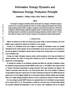
FIG. 1. (A) Ideal bacteriorhodopsin intermediate fractions as a function of time (dashed black line) and apparent fractions in the realistic data (gray continuous lines). The vertical continuous lines mark 65 time points in the realistic data. (B) Experimental difference FT-IR spectra for bR intermediates. (C) Ideal time-resolved FT-IR data for bacteriorhodopsin photocycle. (D) Realistic time-resolved FT-IR data, which includes the instrumental limitations and the presence of realistic random noise.

used a model with six sequential kinetic intermediates with back reactions to describe experimental time-resolved visible spectra:44 1:7 ls

52 ls

130 ls

1:4 ms

1:2 ms

6:4 ls

91 ls

380 ls

7:3 ms

1:5 ms

1:1 ms

K Y L Y M1 Y M2 Y N Y O ! bR

FIG. 2. Time traces and lifetime distributions at (A) 1525 cm1, (B) 1192 cm1, (C) 1186 cm1, and (D) 1631 cm1. Upper row: ideal (gray line) and realistic (black dots) time traces. Second row: MaxEnt (continuous lines) and true (dashed lines with open dots) lifetime distributions. The MaxEnt lifetime distributions were obtained from the ideal time traces. Third row: MaxEnt (continuous lines) and true (dashed lines with open dots) lifetime distributions. The MaxEnt lifetime distributions were obtained from the realistic time traces, using the most probable Bayesian inference about the regularization parameter. Bottom row: Optimum regularization value provided by Bayesian inference with uniform (black line) and Jeffrey’s prior (gray line), generalized cross-validation (GCV), and the L-curve curvature.

The dashed black lines in Fig. 1A represent the ideal intermediate fractions, whereas the continuous gray lines give the apparent fractions, which take into account the limited time-resolution and the pseudo-logarithmic average. The pure intermediate spectra are presented in Fig. 1B. They are experimental difference spectra obtained at a temperature and pH where the different bR intermediates are specially accumulated, normalized by the 1250 cm1 band area.49,71 It is important to stress that we do not claim that these data represent the real intermediate fractions and the pure difference spectra of bR intermediates. We only used these data as a means to create reasonable ideal (Fig. 1C) and realistic noisy (Fig. 1D) synthetic time-resolved FT-IR data, as conceivably realistic as possible. Indeed, the synthetic data in Fig. 1C resembles published experimental data.85 Since the kinetic model used to create the synthetic data in Fig. 1 contained six kinetically different intermediates, the time-resolved data also contains six exponential decays. Their macroscopic time constants are 1.364, 33.09, 156.0, 484.0, 1590, and 4246 ls (0.135, 1.520, 2.193, 2.685, 3.201, and 3.628 log s/ls), whereas the DAS are shown in Fig. 3C (see below, gray spectra, which completely overlap with the black spectra). The DAS are made of a combination of pure

intermediate difference spectra, with combination fractions given by the eigenvectors of the kinetic matrix, whereas the macroscopic time constants are the minus reciprocal eigenvalues of the kinetic matrix, which depends on the kinetic model. Also, since the kinetic model contained two spectroscopically degenerate intermediates (M1 and M2) the synthetic data contains only five significant singular values (not shown). Further details are given in the Introduction, in the Methods section, and in the corresponding references. As we have already explained, the number of exponential decays, their time constants and their DAS, and the number of significant singular values represents the only kinetic information we can expect to be able to extract from the time-resolved spectroscopic data without any assumption about the intermediate pure difference spectra or the intermediates fraction evolution with time. MaxEnt-iLT of Ideal and Realistic Data. First, we tested MaxEnt-iLT on the ideal and realistic data. Figure 2 (upper row) shows time traces for both the ideal (gray line) and realistic (filled black circles) noisy data at some selected wavenumbers (column A, 1525 cm1; column B, 1192 cm1; column C, 1186 cm1; and column D, 1631 cm1). For noise-free data the MaxEnt solution is uniquely defined: there is only one maximum entropy lifetime distribution


435

FIG. 3. (A) Contour plot (100 equidistant contour lines are drawn) of the MaxEnt 2D-lifetime distribution obtained from the ideal data (gray contour lines). The boxes made of dashed lines give information about the log s intervals used to obtain the DAS in (C). (B) Absolute cumulative lifetime distribution for the MaxEnt 2D-lifetime distribution (continuous line) and the true 2D-lifetime distribution (dashed line with open circles). Band maxima, corresponding to the MaxEnt time constants are labeled, which are almost in perfect agreement with the actual values. (C) Decay associated spectra (DAS) for the ideal MaxEnt 2D-lifetime distribution in (A) (black line). The DAS are labeled by the time constants obtained in (B). The MaxEnt DAS are in perfect agreement with the true DAS (gray lines, completely hidden by the black lines).

constrained to the data. The MaxEnt solution for noise-free data can be approximately obtained using the algorithm descried in the Methods section (designed for noisy data) using the lower regularization value which allowed the MaxEnt-iLT algorithm to converge. Therefore, being noise free, the analysis of the ideal data is not complicated by the election of the regularization value. Figure 2 (second row) shows the corresponding MaxEnt lifetime distribution (continuous line) and compares it with the true lifetime distribution (open circles with dashed lines). The MaxEnt lifetime distribution is a slightly broader version of the true lifetime distribution. Since the MaxEnt solution preserves all the uncertainties not removed by the data, the broadening in the MaxEnt lifetime distribution informs us about the information lost in the Laplace transform, even in an ideal scenario. In the presence of noise, MaxEnt-iLT output becomes highly dependent on the regularization value used. Now, MaxEnt-iLT does not provide a single solution but a trajectory of solutions (one solution for each regularization value). In the Theoretical Background section we presented a Bayesian maximum entropy method approach for making inferences about the most probable lifetime distribution given the data. The best inference about the solution becomes roughly equivalent to the regularized MaxEnt solution using the regularization parameter with higher posterior probability. Figure 2 (bottom row, Bayesian panel) shows the posterior probability of k as a function of log k, Pr(log kjd, r), for each data time trace. We used two different uninformative priors for k: a Jefreys prior Pr(log k) ¼ cte (gray line), and a uniform prior Pr(log k) } k (black line). We can see than the inferred k is basically independent of the prior probability we assign to k. The value of log k with higher posterior probability, log kMP, is given in the same plot. The realistic noisy time traces were then analyzed by MaxEnt-iLT, using the kMP obtained with the uniform prior. Figure 2 (third row, continuous lines) shows the obtained MaxEnt lifetime distribution, which also corresponds to the

436


Bayesian MaxEnt best inference about the solution. The obtained MaxEnt lifetime distributions provide the correct number of bands (exponential decays) and good estimates of their position (time constants) and area (amplitudes). Although the MaxEnt lifetime distributions in Fig. 2 are in relative agreement with the actual lifetime distributions, it is also evident that there are some discrepancies. It is important to realize why under realistic conditions the MaxEnt lifetime distributions differ from the ideal ones and to know to which degree these differences are predictable. This subject has been treated in detail elsewhere.72 Briefly, there are two sources of errors or distortions involved in the lifetime distributions obtained by MaxEnt-iLT. The first source is caused by the presence of noise in the data. The noise-induced errors manifest themselves as band positions/widths/areas errors for the bands in the lifetime distribution, as well as the appearance of artifactual bands. Noise-induced errors in the band parameters can be estimated from the Bayesian approach to MaxEnt,21 as well as by brute force Monte Carlo methods.72 The same methods also allow the identification of noise-induced artifactual bands. In this way, some of the bands in the lifetime distributions of Fig. 2 (third row) were determined to be nonsignificant (marked with an asterisk), and correctly assigned to be noise-induced features. The second source of errors lies in the MaxEnt bias (or regularization-induced errors). The MaxEnt bias causes artifactual band broadening of the lifetime distribution, band position errors (caused by synergism with neighboring bands), and band position and band area errors for bands at a time constant too fast (or too slow) for the experimental time resolution. These errors have been illustrated in the literature,75,77 but are difficult to predict quantitatively. Recently we introduced the concept of apparent resolution function in MaxEnt, which helps in understanding the MaxEnt bias. It also allows for semi-quantitative predictions of the effect of the MaxEnt bias in any particular solution.72 Besides Bayesian inference, we also implemented some pragmatic methods for the automatic selection of the

regularization value in MaxEnt-iLT: generalized cross-validation, the L-curve, and the discrepancy criterion. Figure 2 (bottom row) shows the application of GCV and the L-curve curvature, together with their recommended log kopt values. Both method recommendations are in good agreement with the Bayesian estimates, providing relatively similar (but somewhat broader) MaxEnt lifetime distributions (not shown). Figure 2 does not include the results of the discrepancy criterion, but, as expected, it recommended over-estimated log kopt values: (A) 3.64; (B) 4.03; (C) 4.03; (D) 3.70; leading to over-smoothed solutions with missing components (not shown). M-MaxEnt-iLT of Ideal Data. Obtaining lifetime distributions from time-traces provides a good insight into the number of decays and time constants present in the time-resolved data. However, the results can depend on the studied wavenumber. It is conceivable that some decays could pass undetected in MaxEnt-iLT if the time traces at which they show maximum amplitude are not analyzed. This limitation can be solved by M-MaxEnt-iLT. M-MaxEnt-iLT provides a lifetime distribution for all the time traces. The output of M-MaxEnt-iLT can be regarded as a 2D-lifetime distribution (lifetime distribution as a function of the wavenumbers) or, conversely, as lifetimeresolved spectra (decay associated spectra as a function of the time constants). We applied M-MaxEnt-iLT to the synthetic data in Fig. 1C. For noise-free data it is quite trivial to obtain the MaxEnt 2Dlifetime distribution. The regularization value should be the lowest one that allows the algorithm to converge to a true maximum entropy solution. The 2D-lifetime distribution can be conveniently represented as a contour plot as a function of the wavenumber and time constant decimal logarithm, log s (see Fig. 3A, gray contour lines). As can be observed, the 2Dlifetime distribution is made of bands. All the bands appear aligned in six different rows, and all the bands in a row have the maximum at the same time-constant value. This kinetic synchronization for all the bands is a direct consequence of the fact that the ideal synthetic data was constructed following a system with six intermediates, although the existence of intermediates was not assumed in the analysis. The DAS can be obtained by integrating the 2D-lifetime distribution between suitable log s limits (see Fig. 3A, dashed boxes).30 For the ideal data, the obtained DAS were in perfect agreement with the true DAS (see Fig. 3C and the caption of Fig. 3). Visual information about the number of exponential components present in the time-resolved data, their time constants, and their heterogeneity can be obtained by integration of the 2D lifetime-resolved data along the wavenumber. To avoid cancellation of the positive and negative amplitudes, this process is better performed in the absolute 2D lifetime-resolved data. We will refer to the resulting lifetime distribution as the absolute cumulative lifetime distribution. The bands in the absolute cumulative lifetime distribution had the maximum at nearly the correct time-constant value (see Fig. 3B). Their bandwidth was ’0.04 log s, instead of zero, due to the limitations of the analysis even for noiseless ideal data. This bandwidth represents the minimum bandwidth in the log s dimension obtainable by MaxEnt-iLT, given the entropy expression in Eq. 7 and our choice of the a priori solution m. M-MaxEnt-iLT of Realistic Data. The realistic synthetic data with random noise was also analyzed with M-MaxEntiLT. In the presence of noise, M-MaxEnt-iLT output becomes

FIG. 4. (A) Bayesian posterior probability of the regularization value in MMaxEnt-iLT. (B) Contour plot of the MaxEnt 2D-lifetime distribution obtained from the realistic noisy data using the most probable regularization value (’100 equidistant contour lines are drawn). (C) Absolute cumulative lifetime distribution for the MaxEnt 2D-lifetime distribution (continuous line) and the true 2D-lifetime distribution (dashed line with open circles). Band maxima, corresponding to the MaxEnt time constants, are labeled, which are in reasonable agreement with the actual values. (D) Decay associated spectra (DAS) obtained after integrating the realistic MaxEnt 2D-lifetime distribution between the given log s values (black lines). The true DAS are also displayed (gray lines).

highly dependent on the regularization value used, as happens for MaxEnt-iLT. We adapted and applied a Bayesian inference to M-MaxEnt-iLT, as well as several ad hoc methods to select the regularization value (see the Methods section). Figure 4A shows the posterior probability of the regularization parameter for M-MaxEnt-iLT. The posterior probability of log k is very narrow, and consequently it is nearly completely unaffected by the prior probability assigned to k. For a uniform prior, the log kMP was at 2.43. Figure 4B shows the MaxEnt 2D-lifetime distribution for kMP, which also corresponds to the best inference about the solution given the assumptions involved. The obtained 2D-lifetime distribution is


437

FIG. 5. Different pragmatic methods to obtain an optimum regularization value in M-MaxEnt-iLT: (A) discrepancy criterion; (B) L-curve, with the Lcurve corner detected by the isoderivative criterion (inset); (C) L-curve method, with the L-curve corner determined as the point of maximum curvature (inset); and (D) generalized cross-validation.

a reasonable approximation to the true 2D-lifetime distribution, with some important discrepancies that will be discussed later. The corresponding absolute cumulative lifetime distribution is shown in Fig. 4C. Six decay components are clearly resolved, roughly at the correct log s value. The first band appears appreciably up-shifted, due to the limited time resolution of the realistic data. Also, bands in the cumulative lifetime distribution appear broader for the realistic noisy data than for the ideal data (compare Fig. 4C and Fig. 3B). Being a cumulative distribution, the actual lifetime band broadening and the band position errors in the 2D-lifetime distribution contribute to this broadening. A tiny artifactual component is observed in Fig. 4C at around 0.9 log s. This artifactual component appears because the cumulative lifetime distribution is obtained in absolute value and noise elements are not cancelled but summed up. Fortunately, real and artifactual components in the cumulative distribution can be easily discriminated by observing their corresponding DAS (see, for instance, Fig. 4D). In spite of the success of Bayesian MaxEnt, some distortions and errors are also evident in the 2D-lifetime distribution in Fig. 4B: band-broadening in the log s dimension, appearance of some noise-induced bands, significant time-constant errors for some bands, and the manifestation of synergism between some bands in the form of bridges connecting them. However, bands appearing at a significantly erroneous time constant are limited to bands with small intensity and/or bands with a time constant in the limit of the time resolution of the time-resolved data. On the other hand, noise-induced bands are of low intensity, appearing mostly with one contour line for a contour plot with nearly one hundred lines (signal-to-noise approximately 100). As already explained, the DAS can be obtained by integrating a 2D-lifetime distribution between suitable log s limits. We show the DAS corresponding to the Bayesian MaxEnt 2D-lifetime distribution in Fig. 4D (black lines). The true DAS are also displayed for comparison purposes (gray lines). The estimated and true DAS are in good agreement. Nevertheless, the first DAS shows a slightly systematic infraestimation of the intensity, related to the already commented-

438


upon bias that MaxEnt introduces in the lifetime components that are too fast for the covered time window. Figure 4D also includes DAS integrated between 0.7 and 1.2 log s and above 3.9 log s, which do not have corresponding true DAS. As expected, these extra DAS contained only noise or had insignificant absorbance. It should be pointed out that the Bayesian formalism can provide confidence limits for the estimated DAS. However, we did not explore that possibility in the present paper. As we already mentioned, several ad hoc methods have been proposed for objective and optimum estimation of the regularization parameter, both in MaxEnt and classical regularization problems (see the Methods section). We adapted and applied these methods to M-MaxEnt-iLT, and the results are displayed in Fig. 5 for (Fig. 5A) the discrepancy criterion, (Figs. 5B and 5C) the L-curve, and (Fig. 5D) generalized crossvalidation. The L-curve (log kopt ¼ 2.98 and 2.90) and generalized cross-validation (log kopt ¼ 2.70) suggest a log kopt close to the Bayesian most-probable estimate, whereas the discrepancy criterion (log kopt ¼ 4.25) suggest a much higher log kopt. Figure 6 shows the MaxEnt 2D-lifetime distribution obtained with the regularization value recommended by (Fig. 6A) the discrepancy criterion, (Fig. 6B) the L-curve, and (Fig. 6C) GCV. The MaxEnt 2D-lifetime distribution obtained with the regularization value recommended by the discrepancy criterion led to an over-smoothed solution (Fig. 6A), where many bands are lost and the remaining bands show important errors in their time constant, as becomes even more evident in the absolute cumulative lifetime distribution. In contrast, both the L-curve and GCV provided reasonable log kopt values, leading to nice 2D-lifetime distributions. The L-curve estimate provided the cleanest lifetime distribution, with slightly broader bands in the log s dimension, although without compromising band resolution. In comparison, Bayesian inference provided a dirtier 2D-lifetime distribution, although also more detailed. Moreover, the Bayesian absolute cumulative lifetime distribution (Fig. 5D) provided slightly more accurate time-constant estimates than those from the L-curve and GCV (Figs. 6B and 6C). Independent of the method used to select the regularization parameter, the 2D-lifetime distributions provided by MMaxEnt-iLT have at least two shortcomings, which make them more sensitive to noise than conceivably possible. The first deficiency becomes evident after observing Fig. 7A. Figure 7A shows, with the black continuous line, the most probable Bayesian inference for the regularization parameter as a function of wavenumber (with 96% confidence limits in gray lines). There is almost a four orders of magnitude change of the optimum regularization value depending on the wavenumber considered. However, in M-MaxEnt-iLT a single regularization value is used for all the wavenumbers (dashed line shown in Fig. 7A). This leads to an inefficient use of the information available in the data. One way so solve this problem is to implement M-MaxEnt-iLT with the wavenumber variable k value. Figure 7B shows the 2D-lifetime distribution obtained using the higher confidence limit of the Bayesian estimate of kMP as a function of wavenumber. We can see that the 2Dlifetime distribution in Fig. 7B is less noisy and/or more detailed than any of the 2D-lifetime distributions in Fig. 4B or Fig. 6. Even so, the improvement is quite modest. Moreover, the absolute cumulative lifetime distribution (Fig. 7C) is nearly identical to those in Fig. 4C and Fig. 6. In the present case, a

FIG. 7. (A) Most probable inference about the regularization value as a function of wavenumber for the realistic noisy data (black line). The upper and lower confidence intervals for the best inference are also displayed (gray lines). The dashed line shows the wavenumber-independent most probable regularization from Fig. 4A. (B) Contour plot of the 2D-lifetime distribution obtained by MaxEnt using a wavenumber variable regularization value (’100 equidistant contour lines are drawn). The regularization dependence on wavenumber used was the upper confidence interval from Bayesian inference. (C) Corresponding absolute cumulative lifetime distributions (black lines), compared with the true one (dashed lines with open circles).

FIG. 6. Contour plot of the MaxEnt 2D-lifetime distribution obtained from the realistic noisy data in Fig. 1C (’100 equidistant contour lines are drawn). The regularization values used were those recommended by (A) the discrepancy criterion, (B) the L-curve method, and (C) GCV (see Fig. 5). The plots adjacent to the contour plots show the corresponding absolute cumulative lifetime distributions (black lines) and compare them with the true one (dashed lines with open circles).

wavenumber adaptive k value only slightly improves the quality of the MaxEnt 2D-lifetime distribution, although the improvement could be significant in some other instances. It should be noted that for the L-curve, and especially for GCV, log kopt fluctuates too much from wavenumber to wavenumber (not shown). As a consequence, neither method is directly useful for M-MaxEnt-iLT with wavenumber adaptive k. A more serious deficiency of M-MaxEnt-iLT is its inability to include some relevant information into the solution: the time constants in the 2D-lifetime distribution are likely to be the same at different wavenumbers. Ideally, the global character of M-MaxEnt-iLT should be partial, in order to improve the

quality of the 2D-lifetime distributions without compromising the M-MaxEnt-iLT potential to detect non-synchronous relaxations (time constant dependency on wavenumber for a given DAS). We are currently working on including partial global character in the MaxEnt 2D-lifetime distributions. Comparing M-MaxEnt-iLT and GExpNLLS. The direct comparison of both methods under fair conditions is difficult. They require different inputs, make different assumptions, and provide different outputs. M-MaxEnt-iLT requires only the data, a noise distribution function, an entropy function, and a regularization value. The noise distribution and the entropy function can be chosen on theoretical or pragmatic grounds, whereas the regularization value parameter can be automatically and optimally selected by several methods, as shown in the present paper. No assumption or information about the number and form of the decays, or their synchronicity with the wavenumber, is made or required. In fact, even if this information were available, it would be challenging to include it in M-MaxEnt-iLT. As we have shown, M-MaxEnt-iLT output is a 2D-lifetime distribution. From this 2D-lifetime distribution we can deduce in favorable conditions the initially sought information: number and time constants of the exponential decays, their DAS, as well as some information about the distributed/discrete nature of the decays.72 In contrast to M-MaxEnt-iLT, GExpNLLS requires a parametric fitting model (number and form of the decays) and good initial values for the fitting parameters, along with the data and a noise distribution function. The dependence of the GExpNLLS result on the assumed parametric fitting model represents, in our view, the main limitation of GExpNLLS. In principle, a full Bayesian approach to GExpNLLS could allow for an objective selection of the most probable parametric fitting model. Currently, such possibility has been explored


439

only for the selection of the number of decays in ExpNLLS.86 Alternatively, significance tests on the fitting residuals can be used as a guide to select the number of significant exponential decays.87,88 However, the reliability of significance tests in hypothesis and model selection is highly controversial, when not strongly attacked.65,66,68 Being model-independent, singular value decomposition (SVD) could be an attractive alternative method for selecting the number of decays. Unfortunately, the number of significant singular values is not necessarily equal to the number of exponential decays, since some intermediates can be spectroscopically degenerated, or linearly dependent within the noise.10 The selection of the parametric form of the decays is also required. Its objective selection is very difficult, since even choosing between discrete or distributed decaying models presents serious ambiguities.89–91 Finally, the most positive aspect of GExpNLLS is that the output is directly the sought information, although conditioned to the chosen fitting model. According to the above, when the correct fitting model is used we can expect GExpNLLS to perform better than MMaxEnt-iLT. As expected, when the synthetic realistic data were analyzed by G-ExpNLLS using six exponentials (using as starting values for the time constants those provided by MMaxEnt-iLT), the obtained least square time constants and DAS were in better agreement with the correct ones than those given by M-MaxEnt-iLT (not shown). Also, we can expect the resolvability power of M-MaxEnt-iLT to be significantly inferior to GExpNLLS (and roughly similar to ExpNLLS), as suggested by the observation that the bandwidths in the 2Dlifetime distributions provided by M-MaxEnt-iLT are significantly bigger than the asymptotic standard errors of the time constants given by GExpNLLS (and roughly equivalent to those given by ExpNLLS). All these findings should not be surprising and should not be interpreted as an intrinsic superiority of GExpNLLS over M-MaxEnt-iLT. GExpNLLS is making more assumptions about the solution than MMaxEnt-iLT does, namely, six exponential decays are present, the decays are homogeneous (discrete exponentials), the signal at all the wavenumbers decays with the same common time constants, and the decay time constants are close to those provided by M-MaxEnt-iLT. Whenever all these assumptions happen to be correct, as in this case, the results provided by GExpNLLS will be more accurate than the results of MMaxEnt-iLT. Although M-MaxEnt-iLT gives less accurate results, its results are also conditioned to fewer assumptions about the input data. Therefore, it will still provide a good answer when GExpNLLS assumptions do not hold. Moreover, even when the correct fitting model is used, M-MaxEnt-iLT can perform better than GExpNLLS when the data contains systematic errors or correlated noise, as recently reported.94 Nevertheless, we don’t need to regard M-MaxEnt-iLT and GExpNLLS as competitive tools. As proposed for their onedimensional counterparts, they can complement each other.74 In reality, M-MaxEnt-iLT can check the validity of GExpNLLS assumptions and provide initial guesses for the time constants. M-MaxEnt-iLT as a Tool to Test Quantitative Kinetic Models. The M-MaxEnt-iLT method does not provide any

The resolving power of ExpNLLS (highly related to model selection) has been studied elsewhere.86,92,93 On the other hand, for GExpNLLS and MaxEnt-iLT we are not aware of any systematic study on their resolving power.

440


quantitative kinetic models. However, M-MaxEnt-iLT can be a powerful tool to discriminate and test quantitative kinetic models already proposed. Several kinetic models have been proposed for the bR photocycle. Here, we limited ourselves to quantitative models for the wild type bR photocycle at pH ’ 7 and ’ 298 K, covering from K intermediate to bR ground-state recovery.33–35,39,42–44,55,85 Figure 8 gives the intermediate fractions as a function of time predicted by the quantitative kinetic models considered in this paper. The intrinsic rate constants are given in the figure caption. From these quantitative kinetic models it is straightforward to obtain the macroscopic time constants of decay (given by the minus reciprocal of the kinetic matrix eigenvalues), which we collected in Table I. They differ significantly between the different proposed kinetic models, both in the number and the values. Since the macroscopic time constants are experimentally accessible, it seems that most of the models in Table I could be experimentally rejected by comparing the predicted and the experimental macroscopic time constants of decay. However, it is difficult, and can be misleading, to compare the predicted and experimental estimated time constants directly without considering both the corresponding decay amplitudes as well as the ability of the analytical method to retrieve macroscopic time constants from the experimental data. For instance, a model with a predicted but not observed time constant could still be correct if the predicted corresponding amplitude is too low to be detectable by the method of analysis or if it can be merged with some other exponential decay due to analytical limitations. From the proposed kinetic models we constructed realistic noisy synthetic FT-IR time-resolved data in a way equivalent to Fig. 1. Then, the data were analyzed by M-MaxEnt-iLT. The obtained absolute cumulative lifetime distributions are displayed in Fig. 9 (continuous lines). Figure 9 also shows the ideal macroscopic time constant with their expected absolute cumulative amplitudes (open circles with vertical dashed lines). We can see that in several cases, the ideal (open circles) and the resolvable (continuous line) macroscopic time constants differ, which supports our initial concern about kinetic model rejection by direct comparison of predicted time constants and time constants estimated from the lifetime distribution provided by MaxEnt-iLT.45 The same concern should apply for the direct comparison of predicted time constants and the time constants estimated by GExpNLLS.55 Instead, in our view, ‘‘experimental’’ time constants and kinetic model predicted time constants should be compared after being processed by the same method of analysis, in order to take both the data and the method of analysis into account. The comparison method we propose should be as follows. First, we should obtain the most probable 2D lifetime distribution from the data and its corresponding absolute cumulative lifetime distribution. Then, the same analysis should be performed on synthetic realistic data, constructed from quantitative kinetic models and approximated pure intermediate spectra. The realistic data should reproduce the instrumental limitations present in the experiment as accurately as possible. Then, an acceptable kinetic model should present an absolute cumulative lifetime distribution with the same number of bands observed in the absolute cumulative lifetime distribution from the experimental data. Moreover, if the intrinsic rate constants of the proposed kinetic model are correct, an acceptable quantitative kinetic model should give

FIG. 8. Intermediate fractions as a function of time for the various bR kinetic models, further described in the footnote of Table I (dashed black lines). Apparent intermediates fractions, used to construct the realistic time-resolved data analyzed in Fig. 9 (continuous gray lines). We grouped all substate fractions in main states (e.g., M1 and M2 grouped in M, etc). (A) Varo and Lanyi.33 sK!L ¼ 1.3 ls; sL!MI ¼ 20 ls; sL‹MI ¼ 4.5 ls; sMI!MII ¼ 13 ls; sMII!N ¼ 4 ms; sMII‹N ¼ 15 ms; sN!O ¼ 500 ls; sN‹O ¼ 20 ms; sO!bR ¼ 40 ms; sN!bR ¼ 320 ls. (B) Varo and Lanyi.33 sKI!LI ¼ 0.8 ls; sLI!MI ¼ 89 ls; sMI!NI ¼ 4 ms; sNI$OI ¼ fast; sOI!bRI ¼ 1.3 ms; sKII!LII ¼ 5 ls; sLII!MII ¼ 5 ls; sMII!NII ¼ 13 ms; sMII‹NII ¼ 50 ms; sNII$OII ¼ fast; sOII!bRII ¼ 32 ms; [KI]0/[KII]0 ’ 0.9; and sNI‹OI/sNI!OI ¼ sNII‹OII/ sNII!OII ¼ 3 (assumed). (C) Varo and Lanyi.34 sK!L ¼ 1.3 ls; sK‹L ¼ 18 ls; sL!M1 ¼ 35 ls; sL‹M1 ¼ 15 ls; sM1!M2 ¼ 56 ls; sM2!N ¼ 3.5 ms; sM2‹N ¼ 5.9 ms; sN!O ¼ 5 ms; sN‹O ¼ 2.4 ms; sO!bR ¼ 8 ms; sN!bR ¼ 5 ms. (D) Varo and Lanyi.35 sK!L ¼ 0.7 ls; sK‹L ¼ 7 ls; sL!M1 ¼ 15 ls; sL‹M1 ¼ 7.5 ls; sM1!M2 ¼ 40 ls; sM2!N ¼ 1.6 ms; sM2‹N ¼ 4.3 ms; sN!O ¼ 2.3 ms; sN‹O ¼ 5.2 ms; sO!bR ¼ 3.7 ms; sN!bR ¼ 2.2 ms. (E) Gerwert and co-workers.39,85 sK!L ¼ 2 ls; sL!M ¼ 70 ls; sM!N ¼ 5 ms; sM‹N ¼ 11 ms; sN!O ¼ 1.2 ms; sN‹O ¼ 700 ls; sO!bR ¼ 800 ls. (F) Ludmann et al.42 sK!L ¼ 1.6 ls; sK‹L ¼ 6.5 ls; sL!M1 ¼ 5.5 ls; sL‹M1 ¼ 0.9 ls; sM1!M2 ¼ 9.9 ls; sM1‹M2 ¼ slow; sM2!N ¼ 190 ls; sM2‹N ¼ 55 ls; sN!O ¼ 2.4 ms; sN‹O ¼ 9.2 ms; sO!bR ¼ 8.6 ms; sN!bR ¼ 1.1 ms. (G) Hendler et al.43 sKf!Lf ¼ 6 ls; sLf!Mf ¼ 33 ls; sMf!Nf ¼ 1.8 ms; sNf!Of ¼ 480 ls; sOf!bRf ¼ 4.3 ms; sKs!Ls ¼ 6 ls; sLs!Ms ¼ 120 ls; sMs!bRs ¼ 4.3 ms; [Kf ]0/[Ks]0 ’ 1. (H) van Stokkum and Lozier.44 sK!L ¼ 1.7 ls; sK‹L ¼ 6.4 ls; sL!M1 ¼ 52 ls; sL‹M1 ¼ 91 ls; sM1!M2 ¼ 130 ls; sM1‹M2 ¼ 380 ls; sM2!N ¼ 1.4 ms; sM2‹N ¼ 7.3 ms; sN!O ¼ 1.2 ms; sN‹O ¼ 1.5 ms; sO!bR ¼ 1.1 ms. (I) Hendler.55 sK1*!K1 ¼ 350 ns; sK1!L1 ¼ 1.4 ls; sL1!M1 ¼ 37 ls; sM1!N1 ¼ 2.8 ms; sN1!O1 ¼ 510 ls; sO1!bR1 ¼ 7.3 ms; sK2*!K2 ¼ 350 ns; sK2!L2 ¼ 1.4 ls; sL2!M2 ¼ 120 ls; sM2!bR2 ¼ 7.3 ms; [K1 ]0/[K2 ]0 ’ 0.2. (J) Hendler.55

FIG. 9. Absolute cumulative lifetime distributions obtained from different bR photocycle kinetic models. Realistic noisy data was analyzed by M-MaxEntiLT to give absolute cumulative lifetime distributions (continuous line), and compared with the predicted macroscopic time constants and absolute cumulative predicted DAS (dashed line with open circles). See the Table I footnote, as well as the caption of Fig. 8 for model details about the kinetic models. The regularization value used in all cases was log k ¼ 2.7.

bands at positions approximately equal to those observed in the experimental absolute cumulative lifetime distribution. Moreover, for an acceptable quantitative kinetic model, the area of the bands in the absolute cumulative lifetime distribution should also agree with those obtained from the experimental data, as far as the assumed pure intermediate spectra used to create the synthetic data are reasonably similar to the true pure intermediate spectra. Following these steps would allow for a more objective discrimination between data-supported/data-unsupported quantitative kinetic models for the bR photocycle. The same holds for any other complex kinetic system. ‹ sK1*!K1 ¼ 450 ns; sK1!L1 ¼ 760 ns; sL1!M1 ¼ 10 ls; sM1!O1 ¼ 6.9 ms; sO1!bR1 ¼ 18 ms; sK2*!K2 ¼ 450 ns; sK2!L2 ¼ 760 ns; sL2!M2 ¼ 3.7 ms; sM2!N2 ¼ 71 ls; sM2‹N2 ¼ 1.5 ms; sN2!bR2 ¼ 39 ms; sK3*!K3 ¼ 450 ns; sK3!L3 ¼ 760 ns; sL3!M3 ¼ 210 ls; sM3!bR3 ¼ 18 ms; [K1 ]0/[K2 ]0/[K3 ]0 ’ 0.19/0.49/0.32.


441

TABLE I. Predicted macroscopic time constants (minus eigenvalue reciprocals) for bacteriorhodopsin photocycle kinetic models.a A

B

C

D

1.3 [0.10] 2.9 [0.47] 86 [1.93] 190 [2.28] 4 000 [3.61] 18 000 [4.26]

0.79 [0.10] 5.0 [0.70] 89 [1.95] 1 300 [3.10] 4 000 [3.60] 9 300 [3.97] 43 000 [4.63]

0.74 [0.13] 10 [1.01] 330 [2.52] 1 100 [3.05] 2 500 [3.40] 9 400 [3.97]

0.67 [0.18] 4.8 [0.68] 140 [2.15] 710 [2.85] 1 800 [3.26] 3 700 [3.56]

a

E 2 70 310 2 200 7 100

[0.30] [1.85] [2.49] [3.33] [3.85]

F 0.67 [0.17] 1.3 [0.13] 41 [1.61] 96 [1.98] 2 800 [3.44] 6 400 [3.81]

G 6 33 120 480 1 800 4 300

[0.78] [1.52] [2.09] [2.68] [3.26] [3.63]

H

I

J

1.4 [0.13] 33 [1.52] 160 [2.19] 490 [2.68] 1 600 [3.20] 4 200 [3.63]

0.35 [0.46] 1.4 [0.15] 37 [1.57] 120 [2.09] 510 [2.71] 2 800 [3.45] 7 300 [3.86]

0.45 [0.35] 0.76 [0.12] 10 [1.00] 68 [1.83] 210 [2.32] 3 700 [3.57] 6 900 [3.84] 18 000 [4.25] 39 000 [4.60]

The time constants, s, are given in ls [log s/ls]. Numbers underlined are used for duplicated or nearly duplicated eigenvalues. Macroscopic time-constant values were rounded to two significant digits, and their logarithms to two decimals. (A) Varo and Lanyi.33 Data: UV-Vis optical multichannel (350–750 nm, 100 ns–100 ms). Sample: Purple membrane (PM) in polyacrylamide gel, pH 7.0, room temperature. Kinetic model: K!L$MI!MII$N$O!bR and N!bR. (B) Varo and Lanyi.33 Data and sample idem to (A). Kinetic model: KI!LI!MI![N1$OI]!bRI and KII!LII!MII$[NII$OII]!bRII. (C) Varo and Lanyi.34 UV-vis optical multichannel (350–750 nm, 100 ns–600 ms). Sample: PM in solution, pH 7.0, 293 K. Kinetic model: K$L$M1!M2$N$O!bR and N!bR. (D) Varo and Lanyi.35 UV-Vis optical multichannel (350–730 nm, 100 ns–100 ms). Sample: PM in solution, pH 7.0, 298 K. Kinetic model: K$L$M1!M2$N$O!bR and N!bR. (E) Gerwert and co-workers.39,85 Data: stroboscopic FT-IR combined with step-scan FT-IR. Sample: PM hydrated film, pH 6.5, 293 K. Kinetic model: K!L!M$N$O!bR. (F) Ludmann et al.42 Data: UV-Vis flash photolysis (410–650 nm, 300 ns–0.5 s). Sample: PM in polyacrylamide gel, pH 7.0, 298 K. Kinetic model: K$L$M1$M2$N$O!bR and N!bR. (G) Hendler et al.43 Data: UV-Vis optical multichannel (370–660 nm, 10 ls–189 ms). Sample: PM in solution, pH 7.2, room temperature. Kinetic model: bRf !Lf!Mf!N!O!bRf and bRs !Ls!Ms!bRs. (H) van Stokkum and Lozier.44 Data from Xie et al.54 UV-Vis flash photolysis (380–700 nm, 1 ls–100 ms). Sample: PM in solution, pH 7.0, 298K. Kinetic model: K$L$M1$M2$N$O!bR. (I) Hendler.55 Data from Xie et al.,54 at pH 7.0 and 293 K. Kinetic model: bR1 !K1!L1!M1!N!O!bR1 and bR2 !K2!L2!M2!bR2. (J) Hendler.55 Data from Xie et al.,54 at pH 7.0 and 303 K. Kinetic model: bR1 !K1!L1!M2!O!bR1, bR2 !K2!L2!M2!N!bR2 and bR3 !K3!L3!M3!bR3.

CONCLUSION Time-resolved spectroscopic data are habitually fitted to multi-exponential decay models. For normally distributed errors, the obtained least square time constants and DAS will be those with maximum likelihood, or from the Bayesian point of view, those maximizing the probability of the data given an assumed model (number and form of exponential decays). In any case, the dependence of the results on the assumed model is clear, and it will be implicitly transmitted to any conclusion derived, directly or indirectly, from it. It is obviously desirable to not introduce speculative information in the analysis at so early a stage, which can irreversibly bias further conclusions. The maximum entropy method allows consideration of the entire hypothesis domain of the number and form of the exponential decays. Moreover, the maximum entropy method provides solutions that are robust against data error deviation from ideal behavior. The model hypotheses are formulated as (2D) lifetime distributions and compare it with the data after their Laplace transform. No hypotheses are rejected at the first stage, but only rewarded by their agreement with the data (v2 minimization) and multiplicity (entropy maximization). Both terms (v2 minimization and entropy maximization) are weighted by a scalar (regularization value). For each regularization value only one solution (hypothesis) is a MaxEnt solution, i.e., has the maximum multiplicity for a given data agreement. Considering the regularization parameter as an indeterminate parameter, the maximum entropy method provides a trajectory of MaxEnt solutions. The regularization value should be chosen objectively; otherwise, two researchers facing the same data could end with different MaxEnt (2D) lifetime distributions. Moreover, the regularization value should be optimally chosen, in the sense to provide a MaxEnt (2D) lifetime distribution as reliable as possible. In the present paper we used the full Bayesian maximum entropy method to automatically obtain the best inference for the regularization value, for both maximum entropy inversion of the Laplace transform (MaxEnt-iLT) and the multi-

442


spectroscopic channel maximum entropy inversion of the Laplace transform (M-MaxEnt-iLT). We also adapted, to both MaxEnt-iLT and M-MaxEnt-iLT, methods for the automatic selection of the regularization parameter originally developed in classical statistical regularization. Using synthetic realistic data mimicking a complex system, such as the bacteriorhodopsin photocycle, we could conclude that, except for the habitually used discrepancy criterion (v2/N ’ 1), all the proposed methods (L-curve, generalized cross-validation (GCV), and Bayesian inference) provided reliable (2D) lifetime distributions of the data. In conclusion, the analysis of time-resolved spectroscopic data could be made into an automatic procedure. Still, since MaxEnt is a non-parametric method, the MaxEnt 2D-lifetime distribution does not strictly provide the number of decays, their time constants, and DAS. Instead, they should be somehow calculated/assumed given the form of the obtained MaxEnt lifetime distribution. As a consequence, some subjectivity will persist in the analysis. Nevertheless, the subjectivity will not be as dramatic as in (global) exponential least squares and will act at a later step in the analysis. We have also presented the basis of some simple procedures using the objectivity provided by MaxEnt to select quantitative kinetic models supported by the data. ACKNOWLEDGMENT This work was supported by Japan Society for the Promotion of Science Postdoctoral Fellowship for Foreign Researchers (to V.A.L.F.) 1. R. M. Slayton and P. A. Anfinrud, Curr. Opin. Struct. Biol. 7, 717 (1997). 2. C. Ko¨tting and K. Gerwert, Chem. Phys. Chem. 6, 881 (2005). 3. W. A. Eaton, V. Munõz, S. J. Hagen, G. S. Jas, L. J. Lapidus, E. R. Henry, and J. Hofrichter, Annu. Rev. Biophys. Biomol. Struct. 29, 327 (2000). 4. I. H. van Stokkum, D. S. Larsen, and R. van Grondelle, Biochim. Biophys. Acta 1657, 82 (2004). 5. J. F. Nagle, L. A. Parodi, and R. H. Lozier, Biophys. J. 38, 161 (1982). 6. A. P. Demchenko, FEBS Lett. 310, 211 (1992). 7. J. Ross and M. O. Vlad, Annu. Rev. Phys. Chem. 50, 51 (1999). 8. J. Włodarczyk and B. Kierdaszuk, Biophys. J. 85, 589 (2003). 9. J. F. Nagle, Biophys. J. 59, 476 (1991).

10. 11. 12. 13. 14. 15. 16. 17.

18. 19. 20. 21. 22. 23. 24. 25. 26. 27. 28. 29. 30. 31. 32. 33. 34. 35. 36. 37. 38. 39. 40. 41. 42. 43. 44. 45. 46. 47. 48. 49. 50. 51. 52. 53. 54. 55. 56. 57.

A. K. Dioumaev, Biophys. Chem. 67, 1 (1997). I. Szundi, J. W. Lewis, and D. S. Kliger, Biophys. J. 73, 688 (1997). E. R. Henry, Biophys. J. 72, 652 (1997). L. Zimańyi, J. Phys. Chem. B 108, 4199 (2004). R. Bonneau, J. Wirz, and A. D. Zubergu¨hler, Pure Appl. Chem. 69, 979 (1997). J. G. McWhirte and E. R. Pike, J. Phys. A: Math. Gen. 11, 1729 (1978). W. H. Press, S. A. Teukolsky, W. T. Vetterling, and B. P. Flannery, Numerical Recipes in C. The Art of Scientific Computing (Cambridge University Press, New York, 1992). S. F. Gull, ‘‘Bayesian Inductive Inference and Maximum Entropy’’, in Maximum Entropy and Bayesian Methods in Science and Engineering, G. J. Erickson and C. R. Smith, Eds. (Kluwer Academic Press, New York, 1988), pp. 37–52. E. T. Jaynes, Proc. IEEE 70, 939 (1982). S. Sibisi, Nature (London) 301, 134 (1983). S. F. Gull and G. J. Daniell, Nature (London) 272, 686 (1978). S. F. Gull and J. Skilling, Quantified Maximum Entropy MemSys5 User’s Manual (Maximum Entropy Data Consultants Ltd, Suffolk, 1990). J. E. Meier and A. G. Marshall, Anal. Chem. 63, 551 (1991). P. J. Marshall, M. P. Hobson, S. F. Gull, and S. L. Bridle, Mon. Not. R. Astron. Soc. 335, 1037 (2002). J. A. Potton, G. J. Daniell, and D. Melville, J. Phys. D: Appl. Phys. 17, 1567 (1984). A. K. Livesey and J. C. Bronchon, Biophys. J. 52, 693 (1987). A. K. Livesey, P. Licinio, and M. Delaye, J. Chem. Phys. 84, 5102 (1986). R. K. Bryan, Eur. Biophys. J. 18, 165 (1990). J. C. Brochon, Methods Enzymol. 240, 262 (1994). J. C. Bronchon, J. Pouget, and B. Valeur, J. Fluoresc. 5, 193 (1995). V. A. Lo´renz-Fonfrıá and H. Kandori, Appl. Spectrosc. 60, 407 (2006). M. A. Delsuc and T. E. Malliavin, Anal. Chem. 70, 2146 (1998). J. K. Lanyi and G. Va´ro´, Isr. J. Chem. 35, 365 (1995). G. Va´ro´ and J. K. Lanyi, Biochemistry 29, 2241 (1990). G. Va´ro´ and J. K. Lanyi, Biochemistry 30, 5008 (1991). G. Va´ro´ and J. K. Lanyi, Biochemistry 30, 5016 (1991). J. B. Ames and R. A. Mathies, Biochemistry 29, 7181 (1990). J. F. Nagle, Photochem. Photobiol. 54, 897 (1991). R. H. Lozier, A. Xie, J. Hofrichter, and G. M. Clore, Proc. Natl. Acad. Sci. U.S.A. 89, 3610 (1992). G. Souvignier and K. Gerwert, Biophys. J. 63, 1393 (1992). G. Va´ro´ and J. K. Lanyi, Biochemistry 34, 12161 (1995). I. Chizhov, D. S. Chernavskii, M. Engelhard, K. H. Mueller, B. V. Zubov, and B. Hess, Biophys. J. 71, 2329 (1996). K. Ludmann, C. Gergely, and G. Va´ro´, Biophys. J. 75, 3110 (1998). R. W. Hendler, R. I. Shrager, and S. Bose, J. Phys. Chem. B 105, 3319 (2001). I. H. M. van Stokkum and R. H. Lozier, J. Phys. Chem. B 106, 3477 (2002). A. Lukaćs and E. Papp, J. Photochem. Photobiol. B 77, 1 (2004). R. I. Shrager and R. W. Hendler, J. Phys. Chem. B 107, 1708 (2003). J. Hofrichter, E. R. Henry, and R. H. Lozier, Biophys. J. 56, 693 (1989). B. Borucki, H. Otto, and M. P. Heyn, J. Phys. Chem. B 103, 6371 (1999). C. Zscherp and J. Heberle, J. Phys. Chem. B 101, 10542 (1997). C. Gergely, L. Zimańyi, and G. Va´ro´, J. Phys. Chem. B 101, 9390 (1997). C. Ruckebusch, L. Duponchel, J. P. Huvenne, and J. Saurina, Vib. Spectrosc. 35, 21 (2004). R. Mauer, J. Vogel, and S. Schneider, Photochem. Photobiol. 46, 247 (1987). K.-H. Mu¨ller, H. J. Butt, E. Bamberg, K. Fendler, B. Hess, F. Siebert, and M. Engelhard, Eur. Biophys. J. 19, 241 (1991). A. H. Xie, J. F. Nagle, and R. H. Lozier, Biophys. J. 51, 627 (1987). R. W. Hendler, J. Phys. Chem. B 109, 16515 (2005). G. I. Groma, R. A. Bogomolni, and W. Stoeckenius, Biochim. Biophys. Acta 1319, 59 (1997). L. Zimańyi, J. Saltiel, L. S. Brown, and J. K. Lanyi, J. Phys. Chem. A 110, 2318 (2006).

58. B. U. Klink, R. Winter, M. Engelhard, and I. Chizhov, Biophys. J. 83, 3490 (2002). 59. R. Rammelsberg, G. Huhn, M. Lu¨bben, and K. Gerwert, Biochemistry 37, 5001 (1998). 60. C. Ro¨dig, I. Chizhov, O. Weidlich, and F. Siebert, Biophys. J. 76, 2687 (1999). 61. D. J. C. MacKay, Neural Comp. 4, 415 (1992). 62. D. J. C. MacKay, Neural Comp. 4, 698 (1992). 63. D. J. C. MacKay, Neural Comp. 11, 1035 (1999). 64. P. C. Gregory, Bayesian Logical Data Analysis for the Physical Science (Cambridge University Press, Cambridge, New York, Melbourne, Madrid, Cape Town, Singapore, Saõ Paulo, 2005). 65. E. T. Jaynes, Probability Theory: The Logic of Science (Cambridge University Press, Cambridge, New York, Melbourne, Madrid, Cape Town, 2003). 66. D. J. C. MacKay, Information Theory, Inference and Learning Algorithms (Cambridge University Press, Cambridge, New York, Melbourne, Madrid, Cape Town, 2003). 67. E. T. Jaynes, ‘‘Where do we stand on maximum entropy?’’, in The Maximum Entropy Formalism, R. D. Levine and M. Tribus, Eds. (MIT Press, Cambridge, 1978), pp. 15–118. 68. T. J. Loredo, ‘‘From Laplace to supernova SN 1987A: Bayesian inference in astrophysics’’, in Maximum Entropy and Bayesian Methods, P. F. Fouge`re, Ed. (Kluwer Academic Publishers, Dordrecht, 1990), pp. 81–142. 69. A. Caticha and R. Preuss, Phys. Rev. E 70, 046127(1–12) (2004). 70. M. P. Hobson and A. N. Lasenby, Mon. Not. R. Astron. Soc. 298, 905 (1998). 71. H. Kandori, Biochim. Biophys. Acta 1460, 177 (2000). 72. V. A. Lo´renz-Fonfrıá and H. Kandori, Appl. Spectrosc. 61, 74 (2007). 73. J. Skilling and R. K. Bryan, Mon. Not. R. Astron. Soc. 211, 111 (1984). 74. P. J. Steinbach, R. Ionescu, and C. R. Matthews, Biophys. J. 82, 2244 (2002). 75. A. T. N. Kumar, L. Zhu, J. F. Christian, A. A. Demidov, and P. M. Champion, J. Phys. Chem. B 105, 7847 (2001). 76. D. Lavalette, C. Tetreau, J. C. Brochon, and A. Livesey, Eur. J. Biochem. 196, 591 (1991). 77. J. M. Shaver and L. B. McGown, Anal. Chem. 68, 9 (1996). 78. P. Sengupta, K. Garai, J. Balaji, N. Periasamy, and S. Maiti, Biophys. J. 84, 1977 (2003). 79. N. P. Galatsanos and A. K. Katsaggelos, IEEE Trans. Image Proc. 1, 322 (1992). 80. P. C. Hansen, SIAM Rev. 34, 561 (1992). 81. P. C. Hansen, SIAM J. Sci. Comput. 14, 1487 (1993). 82. P. C. Hansen, Rank-Deficient and Discrete Ill-Posed Problems: Numerical Aspects of Linear Inversion (Society for Industrial and Applied Mathematics, Philadelphia, 1998). 83. G. H. Golub, M. Heath, and G. Wahba, Technometrics 21, 215 (1979). 84. A. Ruhe and P. A. Wedin, SIAM Rev. 22, 318 (1980). 85. K. Gerwert, ‘‘Molecular Reaction Mechanism of Proteins Monitored by Time-Resolved FT-IR Difference Spectroscopy’’, in Handbook of Vibrational Spectroscopy, J. M. Chalmers and P. R. Griffiths, Eds. (John Wiley and Sons Ltd, Chichester, 2002). 86. G. L. Bretthorst, W. C. Hutton, J. R. Garbow, and J. J. H. Ackerman, Concepts Magn. Reson. Part A 27, 64 (2005). 87. R. I. Shrager and R. W. Hendler, J. Biochem. Biophys. Methods 36, 157 (1998). 88. M. Straume and M. L. Johnson, Methods Enzymol. 210, 87 (1992). 89. D. R. James and W. R. Ware, Chem. Phys. Lett. 120, 455 (1985). 90. D. B. Marshall, Anal. Chem. 61, 660 (1989). 91. A. Vix and H. Lami, Biophys. J. 68, 1145 (1995). 92. A. A. Istratov and O. F. Vyvenko, Rev. Sci. Instrum. 70, 1233 (1999). 93. Zˇ. Bajzer, T. M. Therneau, J. C. Sharp, and F. G. Prendergast, Eur. Biophys. J. 20, 247 (1991). 94. S. Lu¨deke, V. A. Lo´renz Fonfrıá, F. Siebert, and R. Vogel, Biopolymers 83, 159 (2006).


443

Bayesian Maximum Entropy (Two-Dimensional ...

Bayesian Maximum Entropy (Two-Dimensional ...

Suggest Documents

Bayesian Inductive Inference and Maximum Entropy

Using Bayesian Analysis and Maximum Entropy

Maximum Probability and Relative Entropy Maximization. Bayesian ...

Bayesian/Maximum entropy analysis of ...

On Bayesian Inference, Maximum Entropy and ... - Semantic Scholar

Maximum Entropy and Bayesian Inference for the ... - Semantic Scholar

Bayesian Maximum Entropy Based Algorithm for Digital X-ray ...

Eliciting vague but proper maximum entropy priors in Bayesian ...

Maximum Entropy - Wolfram

maximum entropy method - Hindawi

Maximum Entropy Wave functions

Pontryagin Maximum Principle and Maximum Entropy ...

Maximum-entropy model - Google Sites

Maximum Entropy Discrimination Denoising Autoencoders

Determination of Maximum Entropy Probability

Information Entropy Dynamics and Maximum

Maximum Entropy and the Lottery.

Domain Adaptation of Maximum Entropy

Maximum entropy distributions on graphs

maximum entropy flow networks - OpenReview

Maximum Entropy Reconstruction Methods in

Fact-Checking Ziegler's Maximum Entropy

Information Entropy Production of Spatio-Temporal Maximum Entropy

The Entropy of the Universe and the Maximum Entropy ... - ANU