into different time âslicesâ and assign one complete static BN to each slice. The time ... If the nodes for slice at time t is dependent only on nodes from slice t-1,.
BAYESIAN NETWORK REPRESENTING SYSTEM DYNAMICS IN RISK ANALYSIS OF NUCLEAR SYSTEMS By Athi Varuttamaseni
A dissertation submitted in partial fulfillment of the requirements for the degree of Doctor of Philosophy (Nuclear Engineering and Radiological Sciences) in The University of Michigan 2011
Doctoral Committee: Professor John C. Lee, Chair Professor Xiuli Chao Professor William R. Martin Assistant Research Scientist Volkan Seker Robert W. Youngblood, Idaho National Laboratory
To my parents
ii
ACKNOWLEDGMENTS I would like to thank members of my doctoral committee all of whom have helped me at various times during my research. I would especially like to express my gratitude to Professor John C. Lee for his supervision, guidance, and assistance on various matters that came up during my work. I would also like to give a special acknowledgement to Timothy Drzewiecki for his extensive help with the RELAP5 code. Finally, I would like to thank my parents for their unwavering support and understanding throughout my endeavors.
iii
TABLE OF CONTENTS
DEDICATION ………………………………………………………………………....... ii ACKNOWLEDGMENTS ……………………………………………………… …….. iii LIST OF FIGURES ………………………………………………………………….. vii LIST OF TABLES …………………………………………………………………….. . x CHAPTER 1 INTRODUCTION ……………………………………………………..
1
1.1
Risk Assessment in the Nuclear Industry ……………………… 1
1.2
Limitations of Static Risk Analysis ……………………………. 3
1.3
Research Scope ………………………………………………… 6
CHAPTER 2 DYNAMIC PROBABILISTIC RISK ANALYSIS …………………… 2.1
2.2
Survey of Available Techniques ……………………………….
8 8
2.1.1
Dynamic Event Tree …………………………………… 9
2.1.2
Monte Carlo Simulation ……………………………….. 10
2.1.3
Discrete Transition Models ……………………………. 10
The Water Tank Problem ……………………………………… 14
CHAPTER 3 THE BAYESIAN NETWORK ……………………………………….. 18 3.1
Static Bayesian Network ……………………………………… 20
3.2
Dynamic Bayesian Network …………………………………... 23
3.3
Continuous Bayesian Network ………………………………… 24
iv
3.4
Application of Bayesian Network to the Water Tank Problem …………………………………….........................… 27
CHAPTER 4 ALTERNATING CONDITIONAL EXPECTATION ……….............
32
4.1
Need for a Code Surrogate …………………………………… 32
4.2
Overview of ACE …………………………………………….. 34
4.3
Data Smoothing ………………………………………………. 36
4.4
A Simple Demonstration of ACE …………………………….. 39
CHAPTER 5 MODELING THE LOSS OF FEEDWATER TRANSIENT …............. 43 5.1
Overview of the Feed and Bleed Operation …………………… 43
5.2
The Zion Plant Description ……………………………………. 49
CHAPTER 6 MODELING OF ZION-1 USING RELAP5 ………………................... 51 6.1
Overview of RELAP5 ………………………………………….. 51
6.2
Modeling of Relevant Physics in RELAP5 ……………………. 53 6.2.1
Conservation Equations ……….………….…….…….... 53
6.2.2
Heat Conduction Representation ………………………. 56
6.3
Modeling of the Zion Plant …………………………………… 57
6.4
Benchmarking of the RELAP5 Model ………………………… 62
CHAPTER 7 DYNAMIC RISK ANALYSIS FOR THE LOSS OF FEEDWATER TRANSIENT ……………………………… 68 7.1
The Dynamic Bayesian Network Model for Feed and Bleed Operation ……………………………………… 69
7.2
RELAP5 Results for Representative Cases …………………. ... 78
7.3
Construction the RELAP5 Surrogates using ACE …………...... 86
v
7.4
Risk Analysis Result for the Loss-of-Feedwater Transient …. . 93
CHAPTER 8 SUMMARY AND CONCLUSIONS ………………………….............. 97 REFERENCES …………………………………………………………............…..... 101
vi
LIST OF FIGURES Figure 2.1
Water tank problem ……………………………………………………............. 15
3.1
A representative Bayesian network ……………………………………............ 20
3.2
A simple dynamic BN expanded over two time slices …………………........... 23
3.3
The BN representation of an AND gate …………………………………......... 25
3.4
A DBN representing the control functions of the water tank problem …........... 28
3.5
Dryout probability calculated using BN and Monte Carlo ………………......... 30
3.6
Overflow probability calculated using BN and Monte Carlo ……………......... 31
4.1
Plots of the dependent variable Y against each of the five independent variables X i …………………………………………………......... 40
4.2
ACE transformations of the dependent and independent variables ………........ 41
4.3
Transformed dependent variable θ as a function of the sum of the transformed independent variables φi …………………………………….......... 42
5.1
Normal pathway of feedwater flow………………………………………......... 44
5.2
Coolant flow path during the feed and bleed operation ……………….. .......... 46
5.3
Emergency guideline associated with the loss of feedwater event ……….. ....... 48
6.1
Nodalization diagram for a representative pressurized water reactor ……......... 58
6.2
Reactor power as a function of transient time …………………………............. 65
6.3
Average coolant temperature as a function of transient time ……………......... 65
6.4
Steam generator void fraction (shell side) as a function of transient time …....... 66 vii
7.1
Bayesian network model for analyzing the F&B scenario …………………..... 71
7.2
Relationship between the maximum fuel clad temperature and the probability of core damage ………………………………………………….... 72
7.3
Peak clad temperature as a function of transient time for the scram delay time of 0 s, 30 s, 60 s, and 90 s ………………………………………………. .. 79
7.4
Primary coolant pressure as a function of time for 30 s scram delay and 2 hours F&B initiation delay …………………………………………….... 82
7.5
Primary coolant temperature as a function of time for 30 s scram delay and a 2 hours F&B initiation delay ………………………………………………... 82
7.6
Peak clad temperature as a function of transient time for the scram delay time of 0 s, 30 s, and 60 s……………………………………………………..... 83
7.7
Peak clad temperature as a function of transient time for the F&B initiation delay of 10 mins, 2 hrs, and 3 hrs after the loss of feedwater ………………..... 84
7.8
Peak clad temperature as a function of transient time for cases where 1 and 2 PORVs successfully opened ………………………………………….. 85
7.9
Feed flow rate (from both high and low pressure injection systems) as a function of primary pressure ………………………………………………. ... 85
7.10
Peak clad temperature as a function of transient time for cases where 33%, 50%, and 100% of the makeup flow (from both the high and low pressure injection systems) are available …………………………………… .... 84
7.11
Peak clad temperature as a function of time for the case where the AFW fails immediately and 20 mins after the loss of feedwater …………………...... 85
7.12
Scatter plots of clad temperature as a function of its independent variables ....... 88
viii
7.13
Scatter plots of coolant temperature as a function of its independent variables .. 88
7.14
Clad temperature as a function of three transformed variables obtained via the ACE algorithm …………………………………………………. ... ….. 89
7.15
Transformed dependent variables as a function of the original for the Primary Coolant Temperature node ……………………………………. .... 89
7.16
Transformed primary coolant temperature as a function of the original variable ………………………………………………………………... 90
7.17
Benchmarking of the coolant pressure surrogate ................................................. 91
7.18
Benchmarking of the clad temperature surrogate ................................................ 92
7.19
Benchmarking of the coolant temperature surrogate ........................................... 93
7.20
Core damage probability as a function of transient time ……………………..... 95
ix
LIST OF TABLES Table 2.1
State space for each controller …………………………………………. .......... 16
2.2
Response of the controller to water level ………………………………. ........... 16
3.1
Conditional probability function for control unit 1 …………………… ............. 30
5.1
Some data for the Zion-1 reactor ……………………………………….. .......... 50
6.1
Setpoints for primary relief valve operation ……………………………. .......... 61
6.2
Comparison of key parameters between the RELAP5 model and the FSAR ……………………………………………………………. ......... 63
6.3
Sequence of event for the loss-of-feedwater transient benchmark ………......... 63
7.1
Flow rate capacity for the low and high pressure injection pumps ……… ......... 73
7.2
Conditional probability table for the SI pumps, assuming a failure probability of 1.37E-6 during 1 hour of operation ………………………. ......... 74
7.3
Adjustable parameters in the Bayesian network model …………………. ......... 75
7.4
Sequence of event following the loss of main feedwater for the reference case …………………………………………………………….. ........ 78
x
CHAPTER 1 INTRODUCTION
1.1
Risk Assessment in the Nuclear Industry
The safe operation of nuclear power plants (NPPs) requires a careful analysis of the consequences of all events that can lead to the release of radionuclides to the environment. The initiating events can range from the failure of key safety systems which may not be immediately detectable to breaks in the primary coolant pipes which can cause damage to the fuel rods within a short period after the accident. Safety analysis, performed both before the construction of the NPPs and during the operation whenever there is a change in the configuration of the plants, can give a quantitative estimate of the risk that accidents or unforeseen events that occur in the plant will lead to offsite consequences. Risk is estimated as a combination of the frequency of the initiating event (for instance, an accident) and the consequence of that event. Risk analysis attempts to determine how the initiating event will progress in time, incorporating the information on the responses of plant personnel and plant equipment. Risk analysis is especially crucial in the nuclear industry since failures of the safety barriers in an NPP may lead to a large release of radiation to the general public. Even if the plant were shut down immediately after an accident, the decay heat generated in the core will still require the operation of the cooling system at an adequate capacity. This level of dependence on the proper function of plant equipment long after shutdown means that there are many possible 1
evolution paths that an initiating event may follow with time. Risk analysis would therefore require a careful prediction of these evolution paths that may result in the undesirable consequences. One of the earliest comprehensive probabilistic risk assessment (PRA) studies of nuclear power plants is WASH-1400 [NRC75]. This study focused on two representative power plants: Surry Power Station Unit 1 (a pressurized water reactor), and Peach Bottom Atomic Power Station Unit 2 (a boiling water reactor). The methodology employed in the study involves combining the fault tree and event tree structures. Fault trees are used to determine the combination of equipment faults that will lead to the failure of plant systems while the event trees are used to determine how different paths in accident evolution can lead to releases of radioactivity. Both the accident sequence and amount and mode of radioactivity releases are grouped into categories to make the analysis manageable. The WASH-1400 is also notable in its use of probabilistic density functions (PDFs) to account for uncertainties of event probabilities [Lee11]. The Zion and Indian Point probabilistic safety assessment studies [Hay99] were conducted around 1982. These studies used the impact vector methodology to simplify the PRA analysis and focused on evaluating the safety of these two plants considering their location near the urban centers. The next major NRC-sponsored PRA study of nuclear power plants occurred a little over a decade after WASH 1400 and is commonly referred to as NUREG-1150 [NRC90b]. This study looks at three additional NPPs in addition to the two studied in WASH-1400. NUREG-1150 examines the accidents starting from any event that can lead to plant damage and follows the evolution until the release of radionuclides to the public
2
and evaluates the consequences of such a release in terms of fatalities. The accident progression event tree (APET) is constructed based on both expert solicitation and simulation codes (which in turn are validated through experiments and operation logs). Accident progression analysis generates a large number of possible accident pathways and is simplified by grouping of the sequence into bins based on the similarity of containment failure mode, probability, and time [Hak08]. The consequence analysis includes the use of radionuclide transport model to predict the spread of radioactivity after containment failure. The final risk integration gives the overall risk of the NPP to the public and is based on both the probability of the accident or malfunction and the consequences associated with them [Lee11].
1.2
Limitation of Static Risk Analysis
One of the limitations of PRA conducted using the static fault tree (FT) and event tree (ET) is that the dynamic response of the plant over time from an initial perturbation is not explicitly represented [Buc08]. The plant dynamics, arising from the interaction of different plant components and from the interaction between the operator and the plant control equipment, cannot be easily predicted during the construction of the static PRA models. The FT/ET approach usually assumes that the accident scenario can be represented as a static grouping of equipment failures or operator failures [Ald92]. Although during the construction of the ET, plant simulations are used to determine the different accident progression paths that the plant may take, it cannot easily account for how parameters such as the time delays in the actuation of safety systems will affect the accident progression. Furthermore, the actions of the automatic control systems depend
3
on both the time-dependent plant parameters and the corrective actions performed by the operator, whose state of knowledge depends on the path of the accident evolution [Kun08, Lab05]. These dependencies make it difficult to predict ahead of time the most likely set of paths in which the accident will evolve. All the possible dependencies of the accident progression mentioned above means that an ideal risk analysis model should account for: (1) the current status of all the relevant plant components, (2) the current status of the plant variables (e.g., pressure and temperature), (3) the current state of knowledge of the operator , (4) the evolution history during the transient of the plant variables, and (5) the response model of both the automatic control systems and the operators. The conventional FT/ET approach can account for the plant component status, the anticipated response of the control systems, and to some extent, the anticipated change in the system variables. However, it ignores how observations made by the operators during the transient can impact the action of the operators. Also, since the response of the plant variables is assumed during the construction of the model, it is based on the most likely plant configuration and configuration changes that the modeler thinks will occur during the accident. Any deviation from these assumptions can lead to changes in the plant response that can render the model invalid [Kop05]. The limitations mentioned above were recognized as far back as in the 1980s, when the concept of dynamic PRA was first developed in detail [Aco92]. However, many of the dynamic PRA techniques that have been proposed have found limited applications in the risk analysis of large, complex systems. For any system, the evolution of the
4
accident can take many different paths, each leading to different undesirable consequences (e.g., core damage) at different times. For large systems, this leads to situations where the complexity of the model grows exponentially with time. Today, detailed dynamic PRA studies are usually done for a smaller subsystems in situations where either the interactions between the process variable and the control systems are critically important, or in cases where human behavior needs to be explicitly modeled. Over the past few years, there have been recognitions that even though static PRA may be insufficient for certain instances where the interaction between plant processes and control systems is important, we often do not need the full power of dynamic PRA methodologies and their associated complications. Several authors have proposed the use of analysis techniques borrowed from the study of artificial intelligence such as the Petri net, artificial neural network, and Bayesian networks to bridge the gap between static and dynamic PRA [Mur02, Por10, Shi08]. Due to their ease of construction and use, graphical methods such as the Bayesian network are especially attractive, especially compared to dynamic PRA methodologies such as the continuous event tree where the construction of the model can be difficult and time consuming. In this dissertation, we will show an extension on the use of the Bayesian network in risk analysis to include the incorporation of the reactor transient code surrogate that can model the dynamics of the reactor during accidents. This linking of the Bayesian network to a fast-running code surrogate will allow risk analysis to be performed in such a way that plant dynamics are directly incorporated into the model. The technique can serve as a bridge between conventional static PRA techniques and a full blown dynamic PRA model.
5
1.3
Research Scope
The research presented in this dissertation will focus on developing an appropriate code surrogate that can accurately represent the behavior of the reactor during a loss-offeedwater (LOFW) transient and linking it to the dynamic Bayesian network model representing the system. Using such a combination will allow the risk analysis to be performed in such a way as to directly account for the dynamics of the plant while maintaining the simplicity (as least for model construction) of static PRA. As mentioned in the previous section, although there exist various dynamic PRA methodologies that do explicitly use system dynamics in the risk analysis, the models using these techniques are either too difficult to construct for large systems or will take too long to solve using today’s computing capabilities. The work presented here is not meant to replace either the static or dynamic PRA. Rather, it is one additional tool that will be available to risk analysts should situations arise where the application of this method will help reduce the burden of the analysis of the safety of dynamic systems. The dissertation will introduce the use of Bayesian network in dynamic PRA over several chapters. Chapter 2 will cover the currently existing methods for dynamic PRA and a simple problem that is commonly used to benchmark new dynamic PRA methodology. It will also describe some previous uses of the Bayesian network in risk analysis. Chapter 3 will describe the theory of the Bayesian network and its extension to the time domain in the form of dynamic Bayesian network (DBN). It will also revisit the simple problem introduced in chapter 2 and shows how this problem can be modeled with the BN. Chapter 4 will introduce the alternating conditional expectation (ACE) technique, a nonparametric regression technique that we will use to develop simplified models (i.e.,
6
the code surrogate) to represent system dynamics during an accident. Chapters 5 and 6 describe the LOFW transient in the pressurized water reactor and a RELAP5 model that is used to study the behavior of the plant during this accident. Chapter 7 presents the results of the risk analysis during the LOFW transient performed with a DBN. The dissertation concludes with chapter 8 with a discussion and ideas for possible extension of the DBN model to include applications in both diagnostics and real time monitoring and updating of data.
7
CHAPTER 2 Dynamic Probabilistic Risk Analysis
2.1
Survey of Available Techniques
Dynamic PRA methodologies that are available today are divided into three broad classes: dynamic event tree, discrete event transition models, and Monte Carlo simulation. The concept of the dynamic event tree extends the static event tree by allowing for branching at arbitrary times during the transient. The branching can be based on both the deterministic changes of the plant process variables and the stochastic transitions (failures) of plant components. The discrete event transition models are based on the discretized state of the plant. The plant state is defined by plant parameters (since these parameters are usually continuous, discretization is required) and the state of the components. Generally, the transition rate between plant states are dependent on the paths that the plant takes to reach the current state. However, keeping track of such a history would require an enormous amount of memory and may be impractical. Therefore, a Markov assumption is usually used. Under this assumption, the probability of transition to another system state is taken to be only dependent on the current state and is independent of how the system reaches the current state. The Monte Carlo simulation represents the plant evolution based on component state transition probabilities. Although the simulation technique can be used to analyze a large variety of dynamic problems with very little assumptions, the main drawback is that 8
a proper sampling technique is required so that rare events (which cover the majority of the accident scenarios in the NPP) are adequately sampled.
2.1.1
Dynamic Event Tree
The dynamic event tree (DET) technique traces the plant state as it evolves in time after an initiating event [Hak08]. Within a certain time interval, the plant state may change from either the stochastic change of the component state (for instance, from an equipment failure) or from the deterministic change of the system variable as governed by plant physics. These deterministic changes can be obtained either from a suitable plant simulation code or from sets of equations governing the physical parameters. For cases where the plant behavior follows the Markov assumption (no dependence on evolution history), the dynamic event tree technique requires little computer memory. However, for cases where the history dependence is important (for instance, cases where observations of the operators play a role in future behavior [Hol99]), storing all the pathways of the accident evolution can be memory intensive. The dynamic event tree technique is also not suitable for sensitivity analysis since any change in the rule set or failure probability will require reanalyzing the entire scenario. The DET methodology has been applied to many problems. Acosta looks at the application in the analysis of the steam generator tube rupture accident [Aco93]. Amendola and Reina applied the idea to the DYLAM code [Coj93] which allows the analysis of small subsystems of the NPP [Ald92]. Labeau [Lab050] extends the idea of the DET to include cases where the branching can be induced by the occurrence of certain stimuli which can be specified during the model construction.
9
2.1.2 Monte Carlo Simulation Direct simulation of the plant behavior involves sampling the possible branching of the plant state based on a specified probability distribution. Unlike the case of the dynamic event tree approach which determines the branching based on a pre-specified set of branching rules, the Monte Carlo simulation samples from a large number of possible branches. This method of sampling leads to one major disadvantage for the Monte Carlo simulation: the difficulty of adequately representing rare events. Appropriate biasing is required to ensure that the result represents all the paths that can lead to core damage during the time interval of interest. Another disadvantage of the Monte Carlo method is that since the final result is an overall probability of reaching a particular end state, it is difficult to gather information about any particular progression pathway. Like the dynamic event tree approach, perturbation of the failure probability usually requires running a completely new simulation. The Monte Carlo simulation technique applied to the water tank demonstration problem is often used in benchmarking other PRA techniques [Mar96]. This problem will be discussed in more detail in section 2.2 and will be used as a benchmarking case for the DBN technique in chapter 3.
2.1.3 Discrete Transition Models The discrete transition model discretizes the system state and component state into different bins [Bel06]. The system evolution itself is represented by the transition of this combined state between different bins. Under the Markov assumption, the transition rate
10
depends only on the current state, and possibly on the transient time, but not on the detail of how the plant reaches its current state. Risk analysis using Markov chains for static systems defines the system state as the state in which the system (i.e., all the components) resides. However, for dynamic systems, we usually make a distinction between the component state and system state. Let x = ( x1 , x2 ,..., xN )T be the vector describing the state of the system variables xk ,
k ∈{1, 2,..., N } . These system variables are plant parameters such as pressure, temperature, and water level that evolve deterministically with time, given a certain plant configuration. The time evolution of the system variables is described by
dx = fi ( x), dt
(2.1)
where fi ( x) is the function describing how the system vector x will evolve with time, given the component state i. Here, the component state refers to a vector describing the state of the plant equipment such as valve position, pump speed, or control rod position. At any given time t, the NPP can be described by the pair ( xt , it ) . Our goal is to find the conditional probability density π ( x, i, t | x0 , i0 , t0 ) , where ( x0 , i0 , t0 ) is the initial state of the plant. If we now assume that the system is Markovian, Eq. (2.1) will satisfy the differential Chapman-Kolmogorov equation: ∂π ( x, i, t | x0 , i0 , t0 ) + ∇ x i( f i ( x)π ( x, i, t | x0 , i0 , t0 ) ) + λi ( x)π ( x, i, t | x0 , i0 , t0 ) ∂t − ∑ p ( j → i | x)π ( x, i, t | x0 , i0 , t0 ) = 0. j , j ≠i
11
(2.2)
Note that the probability p( j → i | x) that the component state vector will change from state j to state i depends on the system state x. An example of this dependence is when the failure probability of a valve depends on the coolant temperature. The transition probability λi ( x) is the probability that the component state leaves state i, given the system state x:
λi ( x) =
∑ p(i → j | x).
(2.3)
j , j ≠i
We should note that in the case where the component failure probability is independent of the system state, we can integrate Eq. (2.2) over all system state x0 . Defining the component transition probability integrated over system states
π (i, t ) = ∫ π ( x, i, t )dx,
(2.4)
Eq. (2.2) becomes d π (i, t ) = − λi π (i, t ) + dt
∑
p ( j → i ) π ( j , t ).
(2.5)
j , j ≠i
Equation (2.5) is the Markov equation commonly used for reliability analysis problems with failure rates that are independent of the deterministic system state [Dev92]. Suppose Eq. (2.1) has the solution x(t ) = gi (t , x0 ). Equation (2.2) can be converted to an integral equation [Dev92, Lab05]:
π ( x, i, t ) = ∫ π ( u , i, t0 ) δ ( x − gi ( t , u ) ) (1 − Fi ( t , u ) ) du
t (2.6) p( j → i | u) 1 + λ u π u , j , t − τ δ x − g τ , u dF τ , u du , ( ) ( ) ( ) ( ) ( ) j i i λi ( x) t∫0 ∫ λ j (u )
where t
Fi ( t , u ) = 1 − e
12
∫
− λi g ( s ,u ) ds t0
.
(2.7)
The integral equation (2.6) can be solved using Monte Carlo methods [Ald92]. To avoid the need for working with continuous state space, we can discretize Eq. (6). We start by defining the cell-averaged probability as:
π k (i, t ) = ∫ π ( x, i, t )dx,
(2.8)
Dk
where Dk is the partition of the state variable x: x ∈ ∪ Dk . Defining the indicator k
function ⎧1, x ∈ D k H k ( x) = ⎨ ⎩0, otherwise
(2.9)
we can integrate Eq. (6) over the cell Dk and obtain
⎛ t ⎞ π k (i, t ) = ∫ π (u, i, t0 ) H k ( gi (t , u ) ) exp ⎜ − ∫ λi gi ( s, u )ds ⎟ ⎜ t ⎟ ⎝ 0 ⎠ ⎛ t ⎞ + ∑ ∫ du ∫ dτπ (u, j , t − τ )H k ( gi (t , u ) ) p( j → i | u ) exp ⎜ − ∫ λi gi ( s, u )ds ⎟ . ⎜ t ⎟ j , j ≠i t0 ⎝ 0 ⎠
(2.10)
t
It is possible to replace the transition probability p( j → i | u ) by p ( j → i |< u >l ) , where
< u >l is the average value of the system state over the cell Dl . Furthermore, we can replace the indicator function H k by its cell average. These approximations lead to an averaged form of Eq. (2.10) which forms the basis of the cell-to-cell mapping technique [Wan04]. The Monte Carlo method and the dynamic event tree approach to solving dynamic PRA problems are not exclusive of one another. A combination of these two methods called the MCDET (Monte Carlo Dynamic Event Tree) was proposed by Hofer and 13
described in [Hof10]. In MCDET, the continuous event tree is discretized by means of Monte Carlo simulations. Discretization here refers to the sampling of the transition time and output state from the continuous event tree. The simulation yields groupings of the sampled paths which can then be analyzed. Recently, interest in the use of graphical techniques in dynamic PRA analysis has led to a new class of techniques [And09]. Dynamic reliability analysis methods that are based on an extension of the static method includes the dynamic fault tree (DFT). A DFT is essentially a conventional static fault tree with several new dynamic gates added [Shi08]. The new gates include the functional dependency (FDEP) gate, the warm and cold spare gates, the priority AND (PAND) gate, and the sequence enforcing (SEQ) gate. The FDEP gate sets the output to true if the trigger is true. The warm and cold spare gates are used for components that are in standby. The PAND gate is true only if the basic event is true in a predetermined order. An extension of the PAND gate to more than two basic events is the SEQ gate. Each of the gates in the DFT can be converted to an equivalent Markov model and solved via the standard methods such as the matrix equation and Monte Carlo simulations [Pou08].
2.2
The Water Tank Problem
The water tank problem and its variation are often used to benchmark new dynamic PRA methodologies [Mar96]. The problem is based on a water tank with a prescribed inlet and outlet flows. The controller controls both flows based on the current water level of the tank.
14
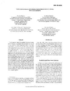
Figure 2.1. Water tank problem. Picture adapted from [Puc08].
Figure 2.1 shows the basic set up of the problem. We start from an initial value where the liquid level is at 0 m. Each of the three control units can be in one of four states shown in Table 1.1. We assume for simplicity that there is no repair and so if the controller fails either to state 3 or state 4, it will remain in that state forever (i.e., states 3 and 4 are absorbing states). Each of the three controllers will adjust its state (between state 1 and 2) based on the water level in the tank, with the goal of maintaining the water level between the lower set point lsp and the high set point hsp. This control behavior is summarized in Table 2.2.
15
Table 2.1. State space for each controller. Controller State Identifier
Controller State Description
1
OFF
2
ON
3
Failed OFF
4
Failed ON
Table 2.2. Response of the controller to water level. Water Level h lsp < h < hsp h < lsp h > hsp
Controller 1 1 2 1
Controller 2 1 2 1
Controller 3 1 1 2
We will assume that the probability of failure into either states 3 or 4 is independent of the original state. The failure time is assumed to be exponentially distributed with the time constants of 219 hr, 175 hr, and 320 hr for controllers 1, 2, and 3, respectively. The pump connected to each of the controllers has the capacity to change the water level by 0.6 m/hr. For this problem, the differential equation governing the water level has a simple analytic solution:
h(t ) = h(t j ) + Q(a1 + a2 − a3 )(t − t j ),
(2.11)
⎧1, if i is in state 1 or 3 ai = ⎨ ⎩0,if i is in state 2 or 4,
(2.12)
where
16
and t j < t is the previous time step. The mission time is 1000 hr. The goal of the problem is to find the time dependent probability that the tank will be in either the dryout ( h < L ) or overflow ( h > H ) state. In the problem described above, the failure rate is independent of the system variable (the water level). This means that classical static PRA methods such as ET/FT and Markov chain can be easily used to solve the problem. However, complications will arise if we allow for cases where the component failure rate depends on the component state or the process variable. In these latter two cases, using static PRA to analyze the problem will present more difficulty. Marseguerra [Mar96] discusses several variations to the water tank problem and how the Monte Carlo approach to dynamic PRA can be used to evaluate the probabilities of overflow and dryout. In chapter 3, we will solve the basic water tank problem with the dynamic Bayesian network.
17
CHAPTER 3 THE BAYESIAN NETWORK
The Bayesian network (BN) is used in many diverse areas of application ranging from medical diagnosis to speech recognition. In this chapter, we will describe the basics of a BN, how they are constructed, and how they can be solved. The theory that is available to support the analysis of the BN is very broad and most will not be needed for a successful application of the BN to certain specific problems. Nevertheless, we will briefly touch on the major developments and applications of the BN so that the versatility of this model can be appreciated. The application of BN to reliability analysis is a relatively recent development. The static form of the network has been applied to study the risk associated with nuclear waste disposal [Lee06] and to study the impact of equipment maintenance on reliability [Web10]. Montani and Portinale [Mon08] developed a reliability tool called RADYBAN which uses the BN to solve dynamic fault tree problems. Boudali [Bou05] looks at the formulation of the continuous form of a temporal BN to calculate the time to failure of an equipment network. In this sense, the BN can be applied to problems that are traditionally analyzed using static fault trees. In their review paper, Langseth [Lan05] discusses how the BN can be used to incorporate the quality of opinions of different experts directly into a risk model.
18
A key feature of the BN that is appealing to many analysts is that the network itself can be constructed based on intuition that is developed through experience without the need for detailed knowledge of the analysis techniques. Although this feature is shared by other graphical techniques, BN is perhaps the most developed in terms of the underlying theoretical framework. In contrast, powerful techniques such as the Markov or semi-Markov models can give similar (sometimes more detailed) results compared to the BN, but with a greater effort required for their construction and analysis. We will divide the presentation of BN theory into several sections. Section 3.1 discusses the basics of the static BN including the interpretation of the independency statement and the use of conditional probability function to quantify the network. Section 3.2 extends the static BN to include a time domain. There are several different ways of including time into the BN, each with their own advantages and disadvantages. Methodologies available to solve the BN is discussed in Section 3.3. Today, there are a number of commercial and open source software available for BN analysis. The most suitable method used to solve the network can depend on the size of the network, the type and amount of data available to populate the network, and the type of information we wish to obtain from the network. In Section 3.4, we will present an application of the BN to solving a dynamic fault tree problem using a continuous formulation of the network. Finally, we will end the chapter by applying the BN to analyze the water tank problem that we presented in Chapter 2.
19
3.1
Static Bayesian Network
A Bayesian network is a directed acyclic graph with nodes representing random variables, and directed arcs linking the nodes, representing conditional dependencies between different variables. It is convenient to classify the nodes as either a parent node or a child node. The parent node is a node that has one or more arc originating from it and pointing towards another node. A child node is a node with incoming arc from another node. A node with no parent is referred to as the root node and a node with no children is the leaf node. For instance, in Figure 3.1, nodes A and B are the parents of node D (this implies D is the child node for nodes A and B). Nodes A and B are root nodes while nodes C and E are leaf nodes. Each parent node N in a BN is associated with the marginal probability distribution P(N) and each child node M has an associated conditional probability P(M|pa(M)), where pa(M) is a set of all the parents of M. Referring again to the BN in Figure 3.1, a complete description of the BN would include, in addition to the graph in Figure 3.1, specification of the probabilities P(A),P(B), P(C), P(C|A), P(D|A,B), and P(E|D).
Figure 3.1. A representative Bayesian network.
20
A graphical representation of the BN like the one in Figure 3.1 shows the conditional independence among the random variables. Generally, a node in a BN is conditionally independent of its non-descendants given the parent nodes. (A node F1 is a descendant of node F2 if there is a directed path from F2 to F1.) In Figure 3.1, the node E is conditionally independent of nodes A and B given that the state of node D is known:
P( E | A, B, D) = P( E | D).
(3.1)
Conditional independence statements like the one in Eq. (3.1) can be used to simplify the joint probability of a system. For any random variables X1, X2,..,Xn we can factorize the joint probability, without any assumption, using the chain rule as: n
P ( X 1 , X 2 ,..., X n ) = ∏ P ( X i | X 1 ,..., X i −1 ).
(3.2)
i =1
However, if we exploit the property of the BN that a variable is independent of its nondescendants given the parents, then Eq. (3.2) reduces to: n
P ( X 1 , X 2 ,..., X n ) = ∏ P ( X i | pa ( X i ) ) .
(3.3)
i =1
The key property of the BN technique is that it factorizes the joint probability distribution. If we have a set of N random variables { X1 ,.., X N } , all the information that we can ever know about these variables can be obtained by knowing the joint distribution function of the variables. However, specifying the joint distribution function is a complicated task. For a discrete random variable, suppose we assume that each of the X i in the set above can be in any one of m possible states. This means that to completely specify the joint distribution, we need to provide m N − 1 numbers. There are several problems associated with this. The most obvious problem is that it will be hard to use
21
this information, especially if m and N are both large. Even with today’s computer, the processing and storage of this amount of information will be slow and expensive. Oftentimes, we do not need all the information that is contained in the joint distribution. However, it is difficult to select the information that we do need without at least some preliminary analysis of the full distribution. The second problem is the difficulty of obtaining the information needed to specify the m N − 1 probabilities. Information from expert elicitation usually does not come in the form of probabilities, and even if they do, most likely not in the form that can be directly entered into the joint distribution. An alternative is to automatically update the
m N − 1 probabilities with data. However, it will take a lot of data, which may not be available, to update the probabilities enough times that the resulting joint distribution accurately represents the true distribution. A BN allows the joint probability distribution to be factored by exploiting the conditional independence relations among the different variables. For instance, consider the BN shown in Figure 3.1. For simplicity, we will assume that each of the 5 nodes in the network can be in one of two states: TRUE or FALSE. If we were to specify the joint conditional distribution P( A = i, B = j, C = k , D = l , E = m) , we would need to specify 25-1=31 probabilities. However, using the conditional independence assumption of Figure 3.1, we can write:
P( A, B, C , D, E ) = P( A) P( B) P(C | A) P( D | A, B) P( E | D).
(3.4)
The number of probabilities needed to specify P( A) is one: we need to only specify
P( A = TRUE) = 1 − P( A = FALSE) . For the term P(C | A) , we only need to specify two 22
probabilities: P(C = TRUE | A = FALSE) and P(C = TRUE | A = TRUE) . Using a similar reasoning for the other terms, we see that the total number of probabilities that we need to specify to determine the RHS of Eq. (3.4) is 1+1+2+4+2=10. Therefore, we see that the assumption of conditional independence can be used to simplify the network. More generally, for a BN with n nodes with k parents or less, the complete specification of the joint distribution requires an order of (2k )n numbers. The unfactorized form of the joint probability requires an order of 2 n numbers.
3.2
Dynamic Bayesian Network
A dynamic Bayesian network (DBN) is a BN that incorporates nodes that can change with time. The simplest way to account for the time dependence is to divide the time line into different time “slices” and assign one complete static BN to each slice. The time dependence then is represented by an arc from the lower numbered slice to a higher numbered one. If the nodes for slice at time t is dependent only on nodes from slice t-1, then we say that the DBN is a two-slice DBN. For a general case, the dependencies may extend to any time slice in the past.
Figure 3.2 A simple dynamic BN expanded over two time slices.
23
A simple DBN is shown in Figure 3.2. For any given slice, node C is completely determined by its parents (nodes A and B). The parent node B at any given slice depends on the value of node A at the preceding slice. The arc linking A at slice 0 to B at slice 1 is referred to as an interslice arc. Interslice arcs indicate the dependence of the nodes that are time dependent. The methods that are available to solve a static BN can be applied to dynamic DBN. The interslice arcs are treated as any regular arcs. Nodes representing the same variables but located in a different time slice are considered to be distinct for the algorithm. The description of the DBN above applies for what is called an instant-based approach to temporal analysis. Another approach of introducing time into the BN is called the interval-based approach. In this approach, the random variables themselves represent events that are time dependent. The time line is usually divided into different disjoint intervals with the node (representing the random variable) defined according to the intervals in which it is located. The DBN models used for our work are all instantbased.
3.3
Continuous Bayesian Network
So far, we have limited our discussion to BNs with nodes that represent discrete random variables. Generally, a BN has no limitation on the type of node it can have. A BN that contains both discrete nodes and continuous nodes are known as mixed or hybrid BN. Most of the inference algorithms that have been developed over the last few decades only apply to a discrete BN or to continuous BN with certain specific distributions.
24
Nevertheless, a continuous BN has several advantages over its counterpart. First, there is no need to discretize the sample space of the variables. This means that common problems that are associated with discrete BNs such as the state space explosion do not exist with the continuous version. Second, since many applications of the BN involve the use of continuous variables, the continuous form of the network is the natural choice to represent these variables. In these instances, the only real reason to discretize the variables is to have access to a greater selection of inference algorithms that can be used. Finally, the solution of continuous BNs can be expressed as integral equations which may be solved by various standard techniques. The ability to write an analytic solution to a BN problem may provide insights into the solution which are more difficult to obtain if we limit to only the numerical relations. In this section, we will present a simple illustration on the use of the continuous BN. The problem is to use the continuous BN formalism to analyze the AND gate in a fault tree. The solution technique is based on the work by Boudali [Bou05] in which he presents the conversion of different dynamic fault tree gates to the BN equivalent. The simple BN model representing an AND gate is shown in Figure 3.3 below.
Figure 3.3. The BN representation of an AND gate.
The variables A and B represents to components, each of which can be in either the operational (FALSE) or failed (TRUE) state. The node C is TRUE only if A and B are 25
both TRUE, otherwise it is FALSE. Let nodes A and B have the time-to-failure distributions f A (t A ) and f B (t B ) , respectively. The function f A (t A ) is the probability density function for component A to fail in the neighborhood of time t A . A similar interpretation applies to f B (t B ) . Next, we need to find the conditional time-to-failure distribution for the node C, given the states of nodes A and B. We note that if node A enters a failed state before node B, then the time to failure of the node C will be equal to the time-to-failure of node B. Conversely, if node B enters the failed state before node A, then the time to failure of node C will be the time to failure of node A. These two statements suggest that the conditional time-to-failure distribution for the node C will be: fC| A, B (tC | t A , t B ) = u (t B − t A )δ (tC − t B ) + u (t A − t B )δ (tC − t A ),
(3.5)
where u(x) and δ ( x) are the unit step function and the Dirac delta function, respectively. The first term on the RHS is nonzero only when A fails before B while the second term is only nonzero when A fails after B. The delta function selects the failure time for C based on the component that fails last. If we now assume that components A and B are independent, we can form the joint time-to-failure density function as: f ABC (a, b, c) = f C| A, B (c | a, b) f A (a) f B (b).
(3.6)
Armed with the joint distribution shown in Eq. (3.5), we can calculate the density function for gate C. This can be done by marginalizing (integrating) Eq. (3.5) with respect to both a and b: f C (c ) = ∫
∞
0
∫
∞
0
f C | A, B (c | a, b) f A (a ) f B (b)dadb
= f A (c) FA (c) + f B (c) FB (c) =
d [ FA (c) FB (c)] , dc
26
(3.7)
where FA ( x) and FB ( x) are the cumulative time-to-failure distribution for components A and B, respectively. Let us compare this solution to the result from the Markov chain analysis. To do this, we will first need to assume that the time-to-failure for both components A and B are exponentially distributed: FA (a) = 1 − e − λAa ,
(3.8)
FB (b) = 1 − e − λBb ,
(3.9)
where λi is the failure rate of component i. Substituting Eqs. (3.8) and (3.9) into Eq.(3.7), we obtain the cumulative time-to-failure distribution of the AND gate: FC (t ) = 1 − e − λAt − e − λBt + e − ( λA + λB )t .
(3.10)
We note that Eq. (3.10) agrees with what we would expect if we approach the problem directly using a Markov chain approach. A similar approach can be used to derive the time-to-failure distribution for other gate types of both the static and dynamic fault trees. For cases involving more than two states, the manipulation of the associated equations becomes much more complicated. For large real world problems, the continuous BNs are usually either discretized and converted to the static BN or solved via Monte Carlo simulations.
3.4
Application of Bayesian Network to the Water Tank Problem
We now consider the water tank problem described in Chapter 2. The objective of this exercise is to calculate the probability of overflow and dryout as a function of time. Figure 3.2 shows the BN associated with this problem. The dependence of the variables vary over two time slices. The states of the three control units determine the changes in water level as governed by Eq. (2.11). The water level in the tank at any time step is the 27
level in the previous step plus any changes based on the configuration of the control units. In the network, this relation is presented by one interslice arc from each of the control unit in the previous slice and another interslice arc from the water level in the previous time step. Since the control units themselves have a constant failure probability, the state of these units at any one time slice depends on the state at the previous slice. The probabilities associated with these interslice arcs are the stochastic failure probabilities of the control units over the time interval represented by the slice. In addition to the possibility of failure, the control units also respond to the water level. These response are represented by the arcs from the water level node to the control units node. However, unlike the arcs representing the control failure, the control arcs are deterministic.
Figure 3.4. A DBN representing the control functions of the water tank problem.
28
The network in Figure 3.4 can be solved by starting at time 0 and solve the BN problem at time 0 with a prescribed initial condition. The result of this analysis will give the values to be used in the calculation of the network in the second slice. This process is repeated over all the time slices. The probability density for the water level in slice 1 can be written as:
P (W #) =
∑
P(W # | W , CU 1, CU 2, CU 3) P(W )
W ,CU 1,CU 2,CU 3
(3.11)
x P(CU 1) P(CU 2) P(CU 3), where the “#” symbol denotes the value in slice 1. At each time slice, the conditional probability function for the control unit i can be expressed in terms of the corresponding probability of the previous time slice: P (CUi #) =
∑
P (CUi # | CUi, W ) P (W ).
(3.12)
CUi ,W
The joint probability density can be summed over all the ancestor nodes: P(W #) =
∑
P(W # | W , CU 1, CU 2, CU 3)P(W )
W ,CU 1,CU 2,CU 3
(3.13)
x P(CU 1) P (CU 2) P (CU 3), The conditional probability function P(CUi # | CUi,W #) that appears in Equation (3.13) is specified by the behavior of the control units as shown in Table 2.2. For instance, the control probability for control unit 1 is shown in Table 3.1. Here, we are assuming that each time slice represents a time step of Δ . The transition probabilities include both the effect of stochastic failures and deterministic controls. If the unit is already in any of the two failed states, we assume that it remains in that state (no repair). At any particular point in time (at any particular slice), the analysis yields a fixed probability for the tank to be at a certain level. These levels are then used to determine whether or not the tank overflows or dries out. The probabilities at each time slice are 29
shown in Figures 3.5 and 3.6. The data from the Monte Carlo simulation are taken from [Mar96] and are generated from 105 simulations. The agreement between the two techniques is very good.
Table 3.1. Conditional probability function for control unit 1. State at t + Δ XU1# OFF FAILED ON λ1Δ 1-2 λ1Δ
State at t W
CU 1 ON
hsp < W < H
ON
0
hsp ≤ W ≤ lsp
ON
L < W < lsp
ON
0 1-2 λ1Δ
1-2 λ1Δ 0
hsp < W < H
OFF
0
1-2 λ1Δ
hsp ≤ W ≤ lsp
OFF
L < W < lsp any any
OFF FAILED OFF FAILED ON
0 1-2 λ1Δ 0 0
FAILED OFF λ1Δ
1-2 λ1Δ 0
λ1Δ λ1Δ λ1Δ λ1Δ λ1Δ
λ1Δ λ1Δ λ1Δ λ1Δ λ1Δ
0 0
0 1
1 0
Dryout Probability (10^-4)
2.5 2.0 1.5 Monte Carlo
1.0
BN 0.5 0.0 0
200
400
600
800
1000
1200
Time (hr)
Figure 3.5. Dryout probability calculated using BN and Monte Carlo. The Monte Carlo result is from [Mar96].
30
Overflow Probability (10^-3)
1.4 1.2 1.0 0.8 0.6
Monte Carlo
0.4
BN
0.2 0.0 0
200
400
600
800
1000
1200
Time (hr)
Figure 3.6. Overflow probability calculated using BN and Monte Carlo. The Monte Carlo result is from [Mar96].
31
CHAPTER 4 Alternating Conditional Expectation
In this chapter, we will introduce the use of the alternating conditional expectation (ACE) to construct a surrogate for any transient analysis code. ACE is a nonparametric, nonlinear multivariate regression technique that determines the optimal functional transformation of both the dependent variable and a set of independent variables such that a linear relationship between the transformed dependent and independent variables is maximized. However, before we discuss ACE in more detail, we will start explaining in Section 4.1 why a code surrogate is needed in our work. Section 4.2 will present the ACE algorithm and some of the physical interpretations that can be associated with the technique. We will also give a brief outline of the algorithm that is used to implement ACE. The final section of this chapter will apply the ACE technique to a simple function so that the benefit of ACE will become clearer.
4.1
Need for a Code Surrogate
Generally, the behavior of a reactor during accident-induced transients depends on the configuration of the plant components which themselves will vary with time. Advanced reactor analysis codes often will have the ability to automatically adjust the state of the components in response to a change in the reactor state variable. For instance, the auxiliary feedwater pumps can be set to automatically turn on when the water level in a 32
steam generator drops below a limit. This capability of these analysis codes to model automatic control means that it is easier for the analyst to focus on specific components important to the study and let the code adjusts the state of the other components. However, in risk analysis, we are interested in finding the overall probability of core damage, given any possible configuration changes of the reactor. This means that we need to specify probabilities of having a component transitioning to different states (e.g., a valve changing its state from OFF to ON) given the state of the plant. To perform this type of analysis, the analysis code needs to be run at all the possible (or at least most likely) combinations of plant component states and then determine how the transient behavior is affected. Considering that a detailed model of a reactor will include many components with many states, the number of all possible combinations is quite large. The run times for these analysis codes for a given case can vary from 10 minutes to several hours. It would take an impractical amount of time to use these codes to study all the possible variations of component states and determine the impact on reactor safety. The idea behind a code surrogate is that we can replace the detailed but slow running analysis code with a somewhat less detailed but much faster representation. A surrogate is basically a function that specifies a deterministic relationship between a dependent variable of interest and a set of independent variables. For instance, we may be interested in a function that expresses the peak clad temperature in terms of coolant flow rate, pressure, and temperature. This surrogate will then be used instead of the simulation code if we want to know how the clad temperature changes as a function of variations in the coolant flow rate, pressure, and temperature.
33
A given surrogate will most likely have a range of applicability. It is important that if we use values of the independent variables that are far outside the range that we use to construct the surrogate, then the surrogate be checked against the original code. The work presented in this dissertation uses several layers of surrogates. In the example above, we pick the flow rate, pressure, and temperature as the independent variables. However, these are not variables over which we have direct control. Therefore, these variables are in turn expressed as a function of other independent variables. The choice of independent variables to use for a given surrogate is made mostly from experience or judgments made from understanding of the basic physics. In this regard, the accuracy of a particular surrogate model will vary from case to case. In the next section, we will present the ACE algorithm which we use to build the various surrogates used in this work. We will defer the discussion of the actual surrogate construction until Chapter 6.
4.2
Overview of ACE
In linear regression analysis over p independent variables, we are interested in finding the coefficients a0 , a1 ,..., a p such that the equation p
Y = a0 + ∑ ai X i + ε
(4.1)
i =1
holds. Here, ε is the error, Y is the dependent variable and X i ’s are the independent variables. Linear regression works well if the relationship between the independent and dependent variables are known to be linear. However, in a more general case, linear regression may give erroneous results. This leads to the development on nonparametric
34
regression techniques which do not assume the functional form of the relationship. These nonparametric techniques are divided into two broad classes: those that perform some kind of transformation on the dependent variable, and those that do not. The ACE model falls into the former class. The ACE algorithm is first proposed by Breiman and Friedman [Bre85] as a way to estimate the optimal transformations of both the dependent and independent variables. By optimal transformation, we mean a transformation that reduces the mean squared error. A different criterion for optimality will lead to a different regression algorithm. The ACE model expresses the transformed function θ of the dependent variable Y in terms of the transformed functions φi of the independent variables X i , i ∈{1, 2,.., p}: p
θ (Y ) = ∑ φ j ( X j ) + ε ,
(4.2)
j =1
where the noise ε has a zero mean and is independent of all the X i ’s. The ACE algorithm aims to minimize the squared error 2
p ⎛ ⎞ er (θ , φ1 ,..., φ p ) = E ⎜ θ (Y ) − ∑ φ j ( X j ) ⎟ . j =1 ⎝ ⎠ 2
(4.3)
For a given value of θ and φ j , j ≠ i, the value of φi that minimizes Eq. (4.3) (i.e., the solution of the minimization problem) is: ⎛
p
⎞
⎝
j , j ≠i
⎠
φi ( X i ) = E ⎜ θ (Y ) − ∑ φ j ( X j ) | X i ⎟ . Likewise, for a fixed φ j , the θ that minimizes Eq. (4.3) is:
35
(4.4)
⎛ p ⎞ E ⎜ ∑ φi ( X i ) | Y ⎟ ⎠ , θ (Y ) = ⎝ i =p1 ⎛ ⎞ E ⎜ ∑ φi ( X i ) | Y ⎟ ⎝ i =1 ⎠
(4.5)
where (•) is the square-norm. The name “alternative conditional expectation” comes from the fact that the ACE algorithm alternates between solving the minimization problem with θ fixed [Eq. (4.4)] and keeping φ j fixed [Eq. (4.5)]. The discussion above can be cast into an algorithmic form shown below [Bre85]: (i) Initialize: set θ (Y ) =
Y − E[Y ] var[Y ]
p ⎛ ⎞ (ii) Obtain new φ : φk ( X k ) = E ⎜ θ (Y ) − ∑ φi ( X i ) | X k ⎟ i =1,i ≠ k ⎝ ⎠
(iii) Obtain new θ : θ (Y ) =
⎛ p ⎞ E ⎜ ∑ φi ( X i ) | Y ⎟ ⎝ i =1 ⎠ ⎡ ⎛ p ⎞⎤ var ⎢ E ⎜ ∑ φi ( X i ) | Y ⎟ ⎥ ⎠⎦ ⎣ ⎝ i =1
(iv) Alternate between (ii) and (iii) until E (θ (Y ) − φ ( X ) ) does not change. 2
4.3
Data Smoothing
Data smoothing is performed when we are interested in finding the behavior of the dependent variable Y as a function of a set of N independent variables X i , i ∈{1,.., N } . The term “smoothing” is used since the output of a smoother generally has less fluctuation (i.e., smoother) than the original variable. In the derivation of the ACE algorithm in Section 4.2, we used the conditional expectation value of the transformed function given the original variable to perform the iteration. However, this works only if
36
we know the joint distribution functions of these variables. Without the distribution functions, we will not be able to calculate the conditional expectation and hence use ACE directly. This is where a smoother comes into play. The results of the smoothing process is used to replace the conditional expectations in the ACE algorithm. Note that since the smoothing process itself is nonparametric, its use in the ACE algorithm does not remove the nonparametric nature of the algorithm. To formalize the notion of data smoothing, we will follow the development in [Bre85]. Suppose we have N sets of p independent variables. Mathematically, we can define this data set to be the set { X1 ,..., X N } whose elements X i is a point in the pdimensional space. For this data set, define F ( X ) to be a space of all real-valued functions Y whose domain is our data set { X1 ,..., X N } . We can think of F ( X ) as a space of all the possible dependent variables. Also define F ( x j ), j ∈ {1, .., p} to be a space of all real-valued functions defined on the set { X 1 j ,..., X Nj } . We can think of F ( x j ) as a space of all possible functions of the independent variable x j . The data smooth S of X on x j is a mapping S : F ( X ) → F ( X j ) that is defined for every data set. For every Y in F ( X ) , we write the corresponding element in F ( x j ) as S (Y | X j ) and its values as S (Y | X kj ). Note that with this definition of smoothing, a linear regression that fits a line through a set of data point can be considered a smoothing technique. However, since linear regression assumes a linear relationship, it is not usually considered to be a real smoother. An example of a simple smoothing technique is a running-mean smoother. Suppose we have a set of N data points of the form ( xi , yi ), i ∈{1,.., N } where xi is the independent variable and yi is the dependent variable. For any given value of xi , we can 37
define a set N S ( xi ) that contains k points closest to the left of xi and k points closest to the right of xi . A running mean smoothing function is then defined as: S ( xi ) = Ave ( y j ). S j∈N ( xi )
(4.6)
The set N S ( xi ) is referred to as the symmetric nearest neighborhood. What we are doing here is essentially averaging the values of the dependent variables within a certain neighborhood. The averaging process will smooth out any variations in the dependent variable. A big disadvantage of this technique is that in cases where the values of the outliers are very different from the values at the interior points, we will lose the information on the behaviors of the dependent variables near those outliers. To alleviate this problem, the running mean smoothing technique can be generalized to use other forms of neighborhood selection (including non-symmetric ones). The choice of the smoothing technique to use determines the output of the ACE algorithm. In this dissertation, we will use the technique originally used in [Bre85] known as a “supersmoother” which basically performs a linear fit within a neighborhood of the point of interest. The size of the neighborhood (i.e., the window width) is allowed to vary, being governed the median of the neighborhood [Fri82]. We will conclude this section by noting that the ACE technique has only been proven to converge if the smoother used in the algorithm is linear. (A linear smoother satisfies S (ay1 + by2 | x) = aS ( y1 | x) + bS ( y2 | x) for any constants a and b.) Nevertheless, the ACE algorithm has been successfully employed in many applications even with a more general choice of smoothers [Bre85].
38
4.4
A Simple Demonstration of ACE
In this section, we will demonstrate the use of the ACE technique to analyze a data set that is synthetically generated from a known functional relationship. This example is adapted from [Wan04]. Consider the equation: eY = 4 + sin(4 X 1 ) + X 2 + X 32 + X 43 + X 5 + 0.1ε .
(4.7)
The variables X i , i ∈{1, 2,3, 4,5} are assumed to be independent with a uniform distribution between -1 and +1. The noise ε is independent of X i and is assumed to be normally distributed with a zero mean and unit variance. We now sample 500 data points from this distribution to generate a set of independent variables and their associated dependent variable Y. With the data set ( X1 , X 2 ,..., X 5 , Y ) generated, we wish to apply the ACE algorithm to try to recover the functional dependence of Y on the X i ’s and compare the results to Eq. (4.7). Of course in practice, we will only have the 500 sample points of the set ( X1 , X 2 ,..., X 5 , Y ) without knowing the relationship between the variables. Faced with an unknown relation between the dependent variable Y and the independent variables X i , i ∈{1, 2,3, 4,5} , one naïve approach may be to look at the scatter plot of Y versus the individual X i with the hope of guessing a functional form of the dependence. Such a plot is shown in Figure 4.1. Looking at the plots, we may perhaps guess that Y may be a sinusoidal function of X 1 while the dependence on the other variables may be linear. If we now apply the ACE algorithm to the data set, we arrive at the relations shown in Figure 4.2. As can be seen from the figure, the ACE technique is able to recover the functional form of the dependent variables: sinusoidal function for X 1 , 39
absolute value function for X 2 , quadratic function for X 3 , cubic function for X 4 , and a linear function for X 5 . The dependent variable Y is transformed to an exponential function, as expected from the relations in Eq. (4.7).
2.5
2
2
1.5
1.5
Y
Y
2.5
1
1
0.5
0.5
0 -1.5
-1
-0.5
0 0
0.5
1
1.5
-1.5
-1
-0.5
0
X1
1.5
2.5
2
2
1.5
1.5
Y
Y
2.5
1
1
0.5
0.5
-1
-0.5
0
0
0.5
1
-1.5
1.5
-1
-0.5
0
0.5
X4
X3
2.5 2
Y
1.5 1 0.5 0 -1.5
1
X2
0 -1.5
0.5
-1
-0.5
0
0.5
1
1.5
X5
Figure 4.1. Plots of the dependent variable Y against each of the five independent variables X i .
40
1
1.5
0.6
1
0.4
0.5
0.2
φ(X2 )
φ(X1 )
-1.5
1.5
0 -1
-0.5
-0.5
0
0.5
1
1.5
0
-1.5
-1
-0.5
-1
-0.4
-1.5 X1
-0.6
0.8 0.6
φ(X 4 )
0.4
φ(X 3)
0.2
-1.5
-1.5
-1
-0.5
0 -1
-0.5
-0.2
-0.2
0
0.5
1
1.5
-0.4 X3
0
0.5
1
1.5
X2
1 0.8 0.6 0.4 0.2 0 -0.2 0 -0.4 -0.6 -0.8 -1 -1.2 X4
0.5
1
1.5
4
1.5
3
1
2
-1.5
1
θ(Y)
φ(X 5 )
0.5 0 -1
-0.5
-0.5
0
0.5
1
1.5
0 -1 0
0.5
1
1.5
2
2.5
-2 -1 -1.5
-3 -4
X5
Y
Figure 4.2. ACE tranformations of the dependent and independent variables.
From the discussion in the previous section, we know that the degree in which ACE can determine the proper correlation can be seen by examining the plot of θ (Y ) vs
∑φ ( X ) . i
i
In the ideal case, the plot should be linear since that is the assumption made in the development of the theory. Figure 4.3 shows that for our example, the relationship is indeed very close to linear.
41
i
y = 1.0111x + 3E-17 R² = 0.9891
4 3 2
θ(Y)
1 -4
0 -3
-2
-1
-1 0
1
2
3
4
-2 -3 -4 Σ φ(Xi)
Figure 4.3. Transformed dependent variable θ as a function of the sum of the transformed independent variables φi .
42
CHAPTER 5 MODELING THE LOSS OF FEEDWATER TRANSIENT
5.1
Overview of the Feed and Bleed Operation
In a pressurized water reactor, the primary means of removing heat from the core during both the normal operation and after shutdown is via the steam generator (SG). Depending on the specific plant, the secondary system is composed of either 3 or 4 closed, two-phase loops that is operated at a pressure of about 800 psi (compared to ~2200 psi for the primary loop). During operation, heat generated from the core is transported via the primary water to the steam generator. The energy is transferred to the feedwater in the secondary loop causing the water to boil. The water-iiiiiiiiiiisteam mixture that is generated is then passed through steam separators which extract the liquid water back into the steam generator. The dried steam is fed to the turbine which extracts energy from the steam (this energy is converted to electricity); the steam passes through the main condenser which converts the steam into liquid water. The water is then pumped back into the steam generator via the feedwater system. The diagram of the secondary system is shown in Figure 5.1. For the reactor during a post-trip, the flow of the steam exiting the steam generator is redirected via the main turbine bypass system and flows directly into the condenser. In the event of a loss of main feedwater in accidents such as feedwater pump failure or leak in the main feedwater loop, the steam generator will receive water from the 43
auxiliary feedwater (AFW) system. The AFW system draws water from various available water sources or from the condensate storage tank and feeds the water into the steam generator. However, unlike the case of the main feedwater, steam produced from the boiling of the AFW is usually vented directly into the atmosphere through the atmospheric dump valve.
Figure 5.1. Normal pathway of feedwater flow. Diagram adapted from [NRC90a].
On the primary side, there are also systems in place to provide backup water needed for heat removal from the core. In the event of a loss of coolant (through a pipe break, for example), the emergency core cooling system (ECCS) can inject borated water from the refueling water storage tank (RWST). The ECCS system comprises three 44
distinct modes of water injection. If the primary system pressure is near the operating pressure, the high pressure safety injection (HPSI) pumps can supply water to the cold leg of the primary loop. These pumps can deliver water at a relatively low rate compared to the other ECCS injection modes, but can operate at a relatively high system pressure. At lower pressure, the low pressure safety injection (LPSI) pumps can provide further injection via the cold leg. There is also a third ECCS component in place called the accumulator or the safety injection tank. This is basically a pressurized tank filled with water that is connected to the primary system. When the primary pressure drops below a setpoint pressure, water will be discharged from the tank into the primary loops. Note that in our discussion in the remainder of the dissertation, the HPSI pump is also referred to as the centrifugal charging pump (CCP) while the LPSI pump is called the SI pump. In the event of the loss of main feedwater coupled with the failure of the AFW system to actuate, the reactor will automatically scram from either the low SG level signal or high primary pressure signal. In either case, the water level in the steam generator will gradually be depleted due to boiling since the decay heat generated by the core will remain relatively high. If no action is taken by the operator, all the secondary water in the SG will eventually be depleted which will lead to a severely degraded heat removal capacity of the secondary system. The primary water will eventually reach saturation temperature and boiling will occur. Ultimately, the core will be uncovered, leading to fuel cladding damage. To prevent the scenario described above from occurring, the feed and bleed (F&B) operation can be initiated to provide an alternate means of heat removal. This involves injecting water into the primary system via the ECCS pumps while venting the steam
45
from the power-operated relief valves (PORVs) located at the top of the pressurizer. The boiling that occurs in the primary will remove the decay heat. The water discharged through the PORVs is stored in the pressurizer quench tank. However, with prolonged F&B operation, the tank will become full, at which point the rupture disks on the tank will burst, releasing the water into the containment sump. In some plants, this water may be pumped back through the LPSI if necessary [Poc02]. Figure 5.2 shows the relevant pathways involved in the F&B operation.
Figure 5.2. Coolant flow path during the feed and bleed operation. Diagram adapted from [NRC90a]. The F&B operation is usually done at the primary pressure near the PORV set point [Rev07]. This pressure is above the shutoff head for the LPSI pumps, therefore only 46
the HPSI pumps will be available. On some PWRs, even the HPSI pump will not have enough power to inject water at high pressure. In this case, the PORVs may be manually opened to relieve the pressure before the feed operation is initiated. This is known as bleed and feed [Rot94]. The emergency guideline for plant operators in the loss of heat sink event is shown in Figure 5.3. The major indicators to initiate the F&B operation include a low steam generator level ( 2335 psi which is the PORV set point). Note that the HPSI pump is first actuated, and if that fails, the procedure calls for the actuation of the LPSI pump. Once at least one pump is verified to be functioning, the PORVs are manually opened to provide the bleed path. The success of the F&B operation depends on the time in which the operation is initiated and on the primary water temperature at the time of initiation [Rev07]. In addition, the number of pumps that are available for the injection, the number of PORVs that can be opened, and the injection rate will be important in determining the heat removal capacity of the F&B operation. In a static event tree that is used to analyze the success criteria of the F&B operation, the dependence of the outcome on the number of PORVs or pumps that are available for the F&B operation can be represented. However, the required feed rate depends on the primary water temperature which is a function of both the F&B initiation delay, the scram delay, and the system pressure. To include these parameters into the analysis, the ET would need to find a limit for these parameters above which the outcome is assumed to be a failure. For example, suppose that a transient simulation indicates that the F&B initiation delay time above 40 minutes will result in the
47
Figure 5.3. Emergency guideline associated with the loss of feedwater event. The flowchart is adapted from [Wes93]. 48
clad temperature exceeding some safe limit. In the event tree, this criteria will be used to test the branching of the accident progression. However, if the plant condition is different from that assumed during the ET construction (for instance, suppose the reactor was not operating at full power), then the 40 minutes limit will no longer be valid. In this case, a new ET with a different branching criterion will be required. If the ET model is aware of the plant state and changes accordingly, then the problem will have been solved. However, it is difficult for the analyst to estimate all the possible conditions of the plant and construct a risk model for every case. One way to alleviate the problem is to couple the risk model with the plant dynamic model. This way, the success or failure criteria can be updated automatically inside the model. In chapter 7, we will show how the code surrogate using ACE (which serves as the plant dynamic model) can be used in conjunction with the Bayesian network (which serves as the risk model) to perform risk assessment in a way that accounts for different plant behaviors.
5.2
The Zion Plant Description
The Zion Station-Unit 1 plant is a 4-loop pressurized water reactor of the Westinghouse design. It is located in northern Illinois and Commonwealth Edison began its operation in 1974. However, it was shut down in 1998. The plant had a rated capacity of 1095 MWe or 3411 MWth. Some basic plant data, including information on the ECCS system, is shown in Table 5.1. The plant is equipped with three trains of AFW pumps, each with enough capacity to feed all four steam generators. Two of these trains are fed by motor driven pumps
49
while the third train is fed by a steam turbine driven pump. Failure of the AFW system means that none of the three trains delivers the auxiliary feedwater at their rated capacity. One feature of the Zion-1 ECCS is that during the recirculation phase, the ECCS pump can realign its suction valve so that water is drawn from the containment sump instead of the RWST. This water is pumped into the inlet of the LPSI pumps which can be injected back into the primary system. For a prolonged F&B operation, the pressurizer sump tank will overflow and the water will be collected in the containment sump. The ability to draw water from the sump means that the available supply of the water for the injection portion of the F&B operation will not be depleted even when the RWST is empty.
Table 5.1. Some data for the Zion-1 reactor. Data from [NRC90a] and [Com82]. Thermal Capacity 3411 MWth Electric Capacity 1095 MWe Number of Fuel Assemblies 193 Number of Fuel Elements in Assembly 264 Number of RCS PORV 2 Number of RCS SRV 3 Number of Charging Pump 2 Centrifugal, 1 Positive Displacement Charging System Capacity - Centrifugal 150 gpm at 2800 psig Charging System Capacity - PD 98 gpm Number of SI Pump 2 SI Pump Capacity 400 gpm at 1084 psig PORV Capacity 64.6 lb/hr/MWth PORV Lowest Setpoint 2335 psig SRV Capacity 129,200 lb/hr SRV Lowest Setpoint 2485 psig
50
CHAPTER 6 Modeling of Zion-1 Using RELAP5
This chapter will introduce RELAP5, the system analysis code that we use to simulate the loss-of-feedwater accident in the Zion-1 nuclear power station. In section 6.1, we will briefly discuss the main features, the representation of key physics, and the modeling capabilities of RELAP5 and how some these capabilities are used in our analysis. In section 6.2, we will describe the modeling of the Zion-1 plant starting from the “typical PWR” input deck that is included in the RELAP5 installation CD and the modifications that were necessary. The “typical PWR” input file itself is based on a detailed Zion-1 model, but it has some important parameters and tables removed due to proprietary considerations. This original model of Zion-1 is designed for the analysis of a loss-ofcoolant (LOCA) accident, so some details that are important for the loss-of-feedwater (LOFW) transient (for instance, the pressurizer safety valves) are not included. Some additions and changes described in section 6.3 are necessary to make the deck applicable to the LOFW transient. In section 6.4, we describe the steady state and transient benchmark of our model against the published results.
6.1
Overview of RELAP5
RELAP5/MOD3.3 (Reactor Excursion and Loss of Coolant Analysis Program) [NRC01] is a one-dimensional analysis code designed for the analysis of the transient behaviors of 51
light water reactors during postulated accident conditions. The code allows the modeler to construct hydrodynamic volumes which can be connected via different types of junction with a prescribed boundary condition such as flow rate or temperature. Conductive heat transfer between several adjacent (but hydrodynamically isolated) volumes can be specified via the use of heat structure. Heat structures are also used in the solid structure that generates heat such as in the fuel rod or pressurizer heater. Using the appropriate connections of the hydrodynamics volume and heat structure, both the primary and secondary systems of the light water reactor can be modeled. Controls of the reactor component can be achieved by the use of trip cards. Trips are basically logic statements that specify when the trip will be true based on a set of inputs. The input to a trip statement can be either other trips or variables that describe the state of a plant component. For instance, a trip logic can be used to represent the pressure where the valve should open or the point in time when a pump should start to coast down. Through the use of appropriate trip combinations, a sophisticated set of control functions and settings can be specified in the RELAP5 model. Internally, the RELAP5 modeling is broken into the fluid model, the heat transfer model, and the reactor kinetics mode. The code uses a two-fluid, six-equation model to describe the fluid behaviors. The two-fluid model allows the treatment of the water/steam mixture and any non-condensable gases that may be present. For reactor kinetics, a point kinetics model is used. Point kinetics treats the neutron flux as a product of the spacedependent and the time-dependent functions. The flux shape function is assumed to be constant in time, while the function describing the magnitude of the flux is time dependent. Heat conduction is modeled using the standard integral formulation of the
52
conduction equation. In addition to the three physics models mentioned above, RELAP5 also allows analysts to build control systems which will automatically control certain plant components such as valves and heaters based on plant variables. Unlike trips whose output are binary, a controller allows the specification of the boundary condition at a node based on values at another node. For instance, the flow rate of the feedwater can be automatically adjusted based on the mass balance of the steam generator. This capability for modeling of the control system allows automatic plant controls and equipment setpoints to be accurately represented.
6.2
Modeling of Relevant Physics in RELAP5
This section will briefly mention some of the main physics models that are used in RELAP5. Since most of these models use the volume and time-averaged value of the variables as the parameter, all the variables listed in this section are cell-averaged quantities and will not be explicitly designated in the individual equations.
6.2.1 Conservation Equations
The description and equations presented in this section are adapted from [Ran89] and [NRC01]. RELAP5 uses a six-equation model to represent the behavior of the fluid. These six equations represent the conservation of mass, momentum, and energy for each of the two phases of the fluid. The conservation of mass for the kth phase is represented by:
∂ 1 ∂ (α k ρ k ) + (α k ρ k vk A) = Γ k , ∂t A ∂x where 53
(6.1)
α k = volume fraction of phase k , ρ k = density of phase k , vk = fluid velocity of phase k , A = cross sectional area, and Γ k = mass generation rate per unit volume for phase k . Here, the subscript k ∈{ f , g} denotes either the fluid or the gas phase. The first term on the LHS represents the change in mass due to a change in density. This change may be due to the thermal expansion of the coolant following an increase in temperature or a contraction due to a pressure drop after a relief valve is opened. The second term describes the balance between mass inflow and outflow from a unit volume. The mass generation term accounts for phase change (boiling or condensation) of the coolant. Note that since there can only be two phases in Eq. (6.1), we also require: Γ f = −Γ g .
(6.2)
Generally, the phasic momentum equations are a set of three equations, representing each of the three directions in a 3-dimensional space. However, with the assumption that the flow is only aligned in one direction, we can neglect the average velocity in the other two coordinates. The conservation of momentum equation in the flow direction becomes, for the gas phase: ∂vg
∂vg ∂P 1 + α g ρg A = −α g A + α g ρ g BX A − (α g ρ g A ) FWG(vg ) α g ρg A ∂x ∂x dt 2 +Γ g A(vgI − vg ) − (α g ρ g A ) FIG(vg − v f ) 2
−Cα gα f ρ A
and for the liquid phase:
54
∂ ( vg − v f ) ∂t
+ vf
∂vg ∂x
− vg
∂v f ∂x
,
(6.3)
∂v f
∂v f ∂P 1 + αf ρf A = −α f A + α f ρ f BX A − (α f ρ f A ) FWF(v f ) αf ρf A ∂x ∂x dt 2 +Γ f A(v fI − v f ) − (α f ρ f A ) FIF(v f − vg ) 2
−Cα f α g ρ A
∂ ( v f − vg ) ∂t
+ vg
∂v f ∂x
− vf
∂vg ∂x
(6.4)
,
where P = pressure, C = coefficient of virtual mass, FWG, FWF = wall frictional drag coefficient for the gas and liquid phases, respectively, FIG, FIF = interphase drag coefficient for the gas and liquid phases, respectively, Bx = body force in the flow direction vgI , v fI = interfacial velocity for the gas and liquid phases, respectively. The terms on the right side of Eqs. (6.3) and (6.4) represent, in the order shown in the equations, the pressure gradient, the body force (such as from pump head), wall friction, momentum transfer due to interphase mass transfer, interphase friction drag, and the force due to mass acceleration (also called the virtual mass). Note that the interphase drag coefficients are linear in the relative phase velocity. The thermal energy conservation equation is:
∂α ∂ 1 ∂ P ∂ (α k ρ kU k ) + (α k ρ kU k vk A) = − P k − (α k vk A) + Qwk + Qik ∂t A ∂x ∂t A ∂x + Γig hk* + Γ w hk' + DISSk , where
55
(6.5)
Qwf , Qwg = phasic wall heat transfer rates per unit volume hg* , h*f = phasic enthalpies associated with bulk interface mass transfer hg' , h'f = phasic enthalpies associated with wall interface mass transfer Γig = vapor generation from energy exchange Γ w = vapor generation due to wall heat transfer effects Qif , Qig = interface heat transfer DISS f , DISSg = phasic energy dissipation (wall friction, pump effects). The first term on the LHS describes the heat added into the control volume (for instance, through a heat structure). The second term represents the net heat flow into the control volume by mean of the motion of the fluid (convective heat transfer). The RHS describes the various looses due to friction or the transfer of energy between the two phases.
6.2.2
Heat Conduction Representation
A heat conduction model is used in RELAP5 to calculate the heat transfer across the solid portion of the reactor components such as across the fuel cladding and across the U-tubes carrying the primary coolant inside the steam generator. The integral form of the heat conduction equation is:
∫ ρ ( x, T )
∂T ( x, t ) dV = ∫ k ( x, T )∇T ( x, t ) • dA + ∫ S ( x, t )dV , ∂t
(6.6)
where
ρ = volumetric heat capacity, k = thermal conductivity, T = temperature, S = heat source.
The surface heat flux q '' required to specify the boundary condition can be calculated as:
56
q '' = h(T − Tsurface ) = −k
∂T , ∂z
(6.7)
where it is assumed that the z vector is the outward normal vector relative to the surface of the boundary. RELAP5 has several correlations built into the code which are used to calculate the heat transfer coefficient h, depending on the flow condition of the hydrodynamics volume. Once the appropriate flow type is selected by the code and the heat transfer coefficient calculated, the surface heat flux in Eq. (6.7) is used as a boundary condition to the heat conduction equation (6.6).
6.3
Modeling of the Zion Plant
Figure 6.1 shows the nodalization of the hydrodynamic volumes of the “typical PWR” input deck that is included as a sample input deck in the RELAP5 installation. The reactor pressure vessel is modeled with 15 volumes comprising the inlet annulus (volumes 300, 305, 310), the downcomer, the downcomer bypass (volumes 315, 320), the lower plenum (volumes 322-325, 330), the upper plenum (volumes 340, 345, 350), the upper head (volumes 355, 356), and the core (volume 335). The core volume is represented with a PIPE component and is subdivided into 6 nodes. Two heat structures are connected to volume 335. The first heat structure, divided into 6 axial and 2 radial segments, models the core barrel. This structure connects volume 335 with the downcomer bypass represented by volume 320. No heat generation is present in this heat structure. The second heat structure represents the fuel pins. It is divided into 6 axial and 16 radial segments. The 16 radial segments represent the fuel material (6 segments), the air gap (2 segments), and the fuel cladding (8 segments).
57
58
Even though Zion-1 is a 4-loop reactor, the “typical PWR” model only has two loops. One of the loops, labeled as the “intact loop”, actually represents a merging of the 3 physical loops. The “broken loop” is one physical loop. This means that parameters such as flow area and flow rate for the “intact loop” is three times that of the “broken loop”. (The reason for this merging is that the original deck is designed for a LOCA analysis and so the loops that do not contain the break are merged to reduce run time.) Except for the pressurizer, the layout of the broken and intact loop is identical. The pressurizer, represented by volume 150, is a PIPE component that is divided into 6 segments. It is connected to the hot leg of the intact loop (it is moved to the broken loop in the final model) via the surge line (volume 152). The top portion of the pressurizer contains an outlet to the PORV (represented by a trip valve 157) which drains into volume 158, representing the quench tank. For each of the steam generators in the two loops, the U-tubes (volume 204 and 108) are modeled with a PIPE component and are each divided into 8 segments. The loss coefficients and hydraulic diameters for these volumes are explicitly specified using appropriate values so that the total flow rate and area computed by the code agree with plant data. The ECCS is represented by two charging pumps (volumes 193 and 293), two LPSI pumps (volumes 191 and 291), and two accumulators (volumes 190 and 290). The sources of the water for all the ECCS pumps are assumed to be infinite for the purpose of the simulation. The dependence of the flow capacity of both the HPSI and LPSI systems are specified via the time-dependent junction which specifies the inject rate as a function
59
of the primary pressure. These junctions are activated by the appropriate trip signal that can be triggered either manually or automatically via a low pressure signal. The secondary side is modeled by 12 volumes. Volumes 170 and 270 have a heat structure connection to volumes 108 and 204, respectively. This connection represents the heat exchanger portion of the steam generator. The heat structure connecting the primary and secondary systems has 16 axial and 8 radial segments. The main feedwater (volumes 182 and 282) and the AFW (volumes 184 and 284) are connected to the steam generator via a branch node (volumes 174 and 274). As in the case of the ECCS, the source of water for these systems is assumed to be infinite. The steam dome is represented by two volumes for each steam generator: a BRANCH component (volumes 180 and 280), and a PIPE volume (volumes 178 and 278) .The steam separator is modeled by the steam separator component (volumes 171 and 271). Five materials are defined in the model: the uranium oxide fuel, the air gap, zircaloy-4 (fuel clad), inconel (U-tubes), and stainless steel (structural components). Each of these materials has a corresponding table for the temperature-dependent thermal conductivity and specific heat capacity. We made modifications to the typical PWR input deck described in the preceding paragraphs to improve the agreement between our model and the data in various published reports for both the steady-state benchmarking and the LOFW transient scenario. 1. The first modification is the addition of the pressurizer heater and spray line. In the original input file, these two components necessary for pressure control are absent and we noticed that it was difficult to achieve a steady state with the correct pressure. The spray
60
line is added so that it draws water from the cold leg (volume 212) and sprays water from the top of the pressurizer (segment 1 of volume 150). Both the heater and the spray are controlled via a proportional controller which takes input from the pressure error at the pressurizer volume. 2. The second modification involves moving the pressurizer from the “intact loop” to the “broken loop”. Recall that the intact loop is really three physical loops merged into one. We felt that the behavior of the pressurizer will be more accurate if it is connected to a loop whose flow condition is closer to the physical loop. 3. The original deck has one PORV to represent the two PORVs that are actually present in the plant. However, for the LOFW transient, there are situations where the PORVs do not have sufficient relief capacity to drain the expanding primary coolant which leads to an increase in the primary pressure large enough so that the code safety valves open. These safety valves were not originally included in the model and had to be added. The control setpoints for the PORVs and the safety relief valves are shown in Table 6.1. Table 6.1. Setpoints for primary relief valve operation. Setpoint Pressure (psia) 2350 2330 2535 2460
PORV open PORV close Relief valve open Relief valve close
4. The control systems for the feedwater system, the steam dump valves, the emergency injection system, and the PORVs were also modified to make them more consistent with the actual behavior of these components. Trip controls were attached to these components so that they actuate when control setpoints are reached. We also had to decrease the pump
61
velocity by 3% to get a better agreement with the steady state values in the final safety analysis report (FSAR) [Com82]. 5. Finally, the control parameters for the steam separator in the steam generator were adjusted to make the separator function properly in a low flow rate situation. The VOVER parameter specifies the void fraction above which the steam will be treated as pure vapor. Similarly, the VUNDER parameter specifies the void fraction limit below which the steam-water mixture will be treated as pure liquid. During the LOFW transient, the steam flow rate drops low enough so that the default values of these parameters were not adequate. We decreased the limit to 1.0E-3 for both parameters.
6.4
Benchmarking of the RELAP5 Model
The benchmarking for both the steady-state case and the LOFW transient case is done to ensure that our Zion-1 model adequately represents the transient behavior during the accident. In the tables and description below, our Zion-1 model will be referred to as the TPWR model. The steady state comparison of the TPWR model and the values from the FSAR is shown in Table 6.2. We see that for most parameters, the agreement is within 1% of the FSAR values. Figures 6.2 through 6.6 compare the LOFW transient results between the TPWR model and the values obtained using the TRAC code as presented in [Dem82]. (The FSAR does not have results for the complete LOFW transient.) Table 6.3 lists the sequence of event for the case used in this benchmarking. The transient starts with the loss of main feedwater, followed by the reactor coolant pump trip and the reactor scram at 1 second. The AFW should come on 15 seconds after the loss of main feedwater but in
62
this case, it fails to do so. At 60 seconds into the transient, the atmospheric relief valve on the secondary side opens in response to high steam generator pressure. Note that the closing of the main steam isolation valve occurs coincident with the reactor scram.
Table 6.2. Comparison of key parameters between the RELAP5 model and the FSAR. FSAR 530 594 9374 2248 653 506 719 972
Vessel Inlet Temp (F) Vessel Outlet Temp (F) Coolant Flow Rate (lbm/s/loop) Pressurizer Pressure (psia) Pressurizer Temp (F) SG Steam Exit Temp (F) SG Pressure, shell side (psia) SG Steam Exit Flow Rate (lbm/s)
TPWR Model 529 593 9431 2252 653 505 719 971
Table 6.3. Sequence of event for the loss-of-feedwater transient benchmark. Time (s) 0.0 1 1 15 60
Event Loss of main feedwater RCP trip Reactor scram AFW system fails Atmospheric relief valves open
Figure 6.2 shows the reactor power as a function of time. Both the TPWR model and the TRAC model that is used in [Dem82] use the American Nuclear Society Standard ANS 5.1 to represent the decay power generated by fission products so we do not expect too much difference in the decay power between the two models. Figure 6.3 shows the average reactor coolant temperature as a function of time. After the RCP trip at 1 second, the primary coolant flow rate decreases as the coolant pumps gradually coast down to about 5% of the flow rate at full power (Figure 6.5). This drop in flow rate will cause the 63
temperature of the coolant to briefly increase (this behavior is called the power-to-flow mismatch in [Dem82]). However, by about 10 minutes into the transient, natural circulation will become the dominant form of primary coolant flow and the temperature will reach its quasi-steady state value. During this time, the primary means of heat removal is through the boiling of the water inventory that remains in the steam generator after the loss of main feedwater. By 80 minutes, the steam generator will have depleted its water inventory and the primary coolant temperature will increase until it reaches saturation temperature. In the period between the dryout of the steam generator and the boiling of the primary coolant, we see an increase of the volume of the coolant due to thermal expansion. This is shown in Figure 6.6, where the pressurizer becomes solid about 100 minutes into the transient. For the most part, the behavior of the reactor during the transient as calculated by our model agrees with the prediction from [Dem82]. The time of the steam dryout is different by about 10-20 minutes but we feel that this difference is small enough so that we can assume our model can adequately model the behavior of Zion-1 during a loss of feedwater transient.
64
Reactor Power (MW)
250 200 150 LANL
100
TPWR
50 0 0
50
100
150
200
250
Time (min)
Primary Coolant Avg Temp (F)
Figure 6.2. Reactor power as a function of transient time.
700 650 600 550
LANL
500
TPWR
450 400 0
50
100 150 Time (min)
200
250
Figure 6.3. Average coolant temperature as a function of transient time.
65
Steam Generator Void Fraction
1 0.9 0.8 0.7 0.6 0.5 0.4 0.3 0.2 0.1 0
LANL TPWR
0
50
100
150
200
250
Time (min)
Pump Mass Flow Rate (lbm/s)
Figure 6.4. Steam generator void fraction (shell side) as a function of transient time.
2500 2000 1500 LANL
1000
TPWR
500 0 0
50
100
150
200
250
Time (s) Figure 6.5. Primary coolant mass flow rate as a function of transient time.
66
Pressurizer Level (%)
120 100 80 60 LANL
40
TPWR
20 0 0
50
100 Time (min)
Figure 6.6. Pressurizer level as a function of transient time.
67
150
CHAPTER 7 DYNAMIC RISK ANALYSIS FOR THE LOSS-OF-FEEDWATER TRANSIENT
In this chapter, we will present the analysis results of loss-of-feedwater transients coupled with the implementation of the F&B operating procedure for the Zion-1 plant. The objective of the analysis is to calculate the time-dependent core damage probability resulting from the LOFW transient. The RELAP5 model used for the analysis is described in chapter 6. Unlike the water tank example of Chapter 2, we will consider several independent variables simultaneously. The number of independent variables presents a problem in that an adequate sampling of all the possible combinations of these variables will take a prohibitively large number of code runs. However, using the appropriate conditional independence assumption, we can construct a Bayesian network model which will allow us to reduce the number of RELAP5 cases necessary for good sampling to a more manageable level. The determination of the conditional independence relationships within a set of variables can be a subjective exercise. As we have shown in Chapter 3, conditional independence and (pair-wise and joint) independence do not imply one another. This means that even for variables that are independent, conditional independence may not hold given some other variable. Complicating the matter further, for a given set of conditional independent variables, it is often possible to construct a Bayesian network in many different ways, depending on the selection of the root nodes. In cases like this, the 68
choice of the appropriate network will be reduced to selecting a model that is the most intuitive given the knowledge of the physics of the problem.
7.1
The Dynamic Bayesian Network Model for Feed and Bleed Operation
The construction a DBN model requires us to make certain assumptions about the conditional independence relations of relevant plant equipment. As we have mentioned in Chapter 3, a DBN model that is constructed without exploiting conditional independencies will have little advantage over other common time-dependent analysis techniques such as the Markov chain in terms of efficiency. Even in situations where it is difficult to make a blanket statement about the conditional independency of a set of variables, we may still be able to construct a useful DBN model if we limit ourselves to an appropriate subset of the state space where the conditional independence assumption does apply (or at least, where conditional dependency is weak enough to ignore). The ability to define suitable sub-region in the state space where a particular DBN model is valid is exploited in the construction of the network shown in Figure 7.1. The dynamic network model in the figure is expanded over two time slices for clarity. Recall from Chapter 3 that one time slice may be thought of as one time step in the discretization of the time variable. For instance, slice 0 can be any time step n while slice 1 is the next time step n+1. We should again note that unlike in numerical analysis, the size of the time step does not play a role in a DBN model. Rather, time difference between any two slice is only important when constructing the inter-slice transition probability.
69
The DBN model in Figure 7.1 has the variable core damage as its only leaf node. For simplicity, we will assume that this node has only two states: failed (representing core damage), and OK (representing no core damage). We are interested in the probability that the node will be in the failed state at any given time during the transient. The parent of Core Damage is the node Clad Temp. The interpretation of this statement is that whether or not core damage occurs depends only on the maximum clad temperature. Note that even though this assumption may not be valid in the general sense (other factors may affect the chance of core damage in other types of accidents), high clad temperature is the dominant indicator of core damage in the LOFW transient which justifies the assumption. The next step is to specify quantitative relationships between the root and child nodes via appropriate conditional probability functions. From the Final Acceptance Criteria [NRC74], the upper temperature limit for Zircaloy clad before clad damage occurs is 2200oF. This motivates our next assumption that any temperature higher than this limit will result in core damage with a probability of 1.0. We will also assume that clad temperatures below 1600oF will not cause core damage. The damage probability increases linearly between these two limits. The relationship described here is shown in Figure 7.2. The triangular probability density function represents the uncertainty in the core damage probability. The corresponding cumulative distribution function is also represented for the RHS ordinate of Figure 7.2. Moving on to the next level in Figure 7.1, we see that Clad Temp has three parents: the primary coolant temperature, primary coolant pressure, and the coolant flow rate. This selection of parent variables will be validated in Section 7.3 when we construct the ACE model for Clad Temp. Unlike the case of the Core Damage node, the
70
71
conditional probability function for Clad Temp is deterministic in the sense that given a value for each of the three parent variables, we assume that we may determine the clad temperature uniquely. Therefore, the conditional “probability” function needs to be constructed based on this deterministic relationship. For our model, this deterministic function is obtained via the ACE regression. As an aside, we note that even though the relationship is deterministic, the use of a probability function also allows us to use “noisy” or “leak” probability which can be used if Clad Temp has additional parents which are
1 0.9 0.8 2.0E-03 0.7 0.6 1.5E-03 0.5 0.4 1.0E-03 0.3 0.2 5.0E-04 0.1 0 0.0E+00 1400 1600 1800 2000 2200 2400 2600 2800 Fuel Clad Temperature (o F) 2.5E-03
CumulativeCore Damage Probability
Core Damage Probability (/oF)
not modeled.
Figure 7.2. Relationship between the maximum fuel clad temperature and the probability of core damage. The node Injection Flow Rate represents the rate at which the injection system (both the high pressure and low pressure injection system) pumps water into the primary system for the feed portion of the F&B operation. The injection rate depends on the 72
number of pumps operating (represented by the nodes No. Low P SI pump and No. Hi P SI pump) as well as the pressure of the primary system. The dependence on the primary pressure arises from the pressure-dependent pumping capacity for the two pump types. As mentioned in Chapter 6, the Zion plant has two types of pump that can be used to inject water into the primary system during normal operation. The high pressure centrifugal charging pump can inject water at a higher primary system pressure but with a relatively low flow rate. The low pressure injection pump has a lower shutoff pressure but can inject water at a higher rate. The pressure dependent flow rates of the these two pump types are shown in Table 7.1. Table 7.1 Flow rate capacity for the low and high pressure injection pumps. Primary pressure (psia) 2620 1685 1529 839 15
High pressure charging pump Liquid Injection Rate (lbm/s) 0 2.65 0.333 7.03 1.00 7.43 9.00 9.30 53.6 9.70
Low pressure SI pump
Figure 7.1 show that the nodes Low P SI pump and No. Hi P SI pump are also parents of the corresponding node in the next time slice. This is represented in the network by arcs originating from slice 0 pointing to nodes in slice 1. The interslice dependency is introduced into the model to account for possible failure of the pumps. For the sake of discussion, let us assume that one time slice represents 1 hour. If the failure rate of the SI pump is 1.37E-3/hr, then the conditional probability table associated with the node Low P SI is shown in Table 7.2. Note that if the pump were ON in the current
73
time step, we assume that it will remain ON in the next time step. If this were not the case, then the last row in Table 7.2 will need to be adjusted accordingly. Table 7.2. Conditional probability table for the SI pump, assuming a failure probability of 1.37E-3 during 1 hour of operation. Time T-Δ OFF ON
Time T OFF 1 1.37E-3
ON 0 0.99863
The root nodes representing the failure time of the auxiliary feedwater system (AFW Fail time), the trip time of the primary coolant pump (RCP Trip Time), the time delay between the loss of feedwater and the reactor scram (Scram Delay), and the F&B initiation delay (Feed Delay and Bleed Delay) are all constant across different time slices. This is intuitive since these variables do not change across time slice. Note that these constant nodes appear under the black line in Figure 7.1 to indicate that they are not specifically part of any one slice but are shared among all slices. In the model, we decided to allow the nodes No. PORV Opened, Low P SI pump and No. Hi P SI pump to vary with each time slice. Physically, this means that the number of pumps and PORVs that are operational may change with time slice. The change in the state of these nodes between different time slices may be caused by stochastic failures, or by deterministic automatic and manual controls. For instance, if we are interested in including human behavior modeling into the network, we may treat the manual control as stochastic to account for variation in operator response time. Human behavior is not considered in this example. To complete the Bayesian network model, we need to specify the root node probability or probability distribution. Table 7.3 shows the values that we
74
use in the model. The choice of the root node and their probabilities are based on [She11], although some numbers are adjusted for our model. We will next describe the significance of some of these variables. In normal circumstance, the reactor is automatically set to scram when the water level in the steam generator falls to about 30% of the narrow range indicator. In the Zion1 plant, this occurs approximately 30 s after the loss of main feedwater if there is no auxiliary feedwater flow. There are situations where the operator may be aware of the feedwater loss before the steam generator water level drops to the automatic trip setting and in these cases, the reactor may be manually tripped before automatic scram occurs. It is also possible that the loss of main feedwater is not abrupt, leading to a longer delay between the start of the loss-of-feedwater event and the steam generator low level signal. To account for these possible scenarios, we model the reactor scram delay time as a uniform distribution between 0 and 90 s. Table 7.3. Adjustable parameters in the Bayesian network model. Description Reactor scram delay F&B initiation delay Number of SI pump available Number of charging pump available Number of PORV opened Delay between feed initiation and bleed initiation Time of RCP trip AFW failure time
Probability Distribution Uniform between 0 and 90 s Lognormal with mean = 4 mins and sigma = 2 mins Failure prob=0.012/demand per pump, Failure rate=1.37E-3/hr Failure prob=0.0078/demand per pump, Failure rate=1.37E-3/hr Failure to open prob=0.014 per valve Normal with mean=20s and sigma=10s Not tripped Failure prob on demand=0.9. Probability of successful actuation but fails