NASA/TM-2002-211944 ARL-TR-2849
Best Practices for Crash Modeling and Simulation Edwin L. Fasanella and Karen E. Jackson U.S. Army Research Laboratory Vehicle Technology Directorate Langley Research Center, Hampton, Virginia
October 2002
The NASA STI Program Office . . . in Profile Since its founding, NASA has been dedicated to the advancement of aeronautics and space science. The NASA Scientific and Technical Information (STI) Program Office plays a key part in helping NASA maintain this important role. The NASA STI Program Office is operated by Langley Research Center, the lead center for NASA’s scientific and technical information. The NASA STI Program Office provides access to the NASA STI Database, the largest collection of aeronautical and space science STI in the world. The Program Office is also NASA’s institutional mechanism for disseminating the results of its research and development activities. These results are published by NASA in the NASA STI Report Series, which includes the following report types: • TECHNICAL PUBLICATION. Reports of completed research or a major significant phase of research that present the results of NASA programs and include extensive data or theoretical analysis. Includes compilations of significant scientific and technical data and information deemed to be of continuing reference value. NASA counterpart of peer-reviewed formal professional papers, but having less stringent limitations on manuscript length and extent of graphic presentations. • TECHNICAL MEMORANDUM. Scientific and technical findings that are preliminary or of specialized interest, e.g., quick release reports, working papers, and bibliographies that contain minimal annotation. Does not contain extensive analysis. • CONTRACTOR REPORT. Scientific and technical findings by NASA-sponsored contractors and grantees.
• CONFERENCE PUBLICATION. Collected papers from scientific and technical conferences, symposia, seminars, or other meetings sponsored or co-sponsored by NASA. • SPECIAL PUBLICATION. Scientific, technical, or historical information from NASA programs, projects, and missions, often concerned with subjects having substantial public interest. • TECHNICAL TRANSLATION. Englishlanguage translations of foreign scientific and technical material pertinent to NASA’s mission. Specialized services that complement the STI Program Office’s diverse offerings include creating custom thesauri, building customized databases, organizing and publishing research results . . . even providing videos. For more information about the NASA STI Program Office, see the following: • Access the NASA STI Program Home Page at http://www.sti.nasa.gov • Email your question via the Internet to
[email protected] • Fax your question to the NASA STI Help Desk at (301) 621-0134 • Telephone the NASA STI Help Desk at (301) 621-0390 • Write to: NASA STI Help Desk NASA Center for AeroSpace Information 7121 Standard Drive Hanover, MD 21076-1320
NASA/TM-2002-211944 ARL-TR-2849
Best Practices for Crash Modeling and Simulation Edwin L. Fasanella and Karen E. Jackson U.S. Army Research Laboratory Vehicle Technology Directorate Langley Research Center, Hampton, Virginia
National Aeronautics and Space Administration Langley Research Center Hampton, Virginia 23681-2199
October 2002
The use of trademarks or names of manufacturers in this report is for accurate reporting and does not constitute an official endorsement, either expressed or implied, of such products or manufacturers by the National Aeronautics and Space Administration or the U.S. Army.
Available from: NASA Center for AeroSpace Information (CASI) 7121 Standard Drive Hanover, MD 21076-1320 (301) 621-0390
National Technical Information Service (NTIS) 5285 Port Royal Road Springfield, VA 22161-2171 (703) 605-6000
Best Practices for Crash Modeling and Simulation I. Abstract II. Introduction - Overview of paper - Objectives III. General Issues in Developing a Crash Model - Reference frame and units - Coordinate frames - Systems of consistent units - Geometry Model - Engineering drawings - Photographic methods - Photogrammetric survey - Hand measurements - Existing finite element model - Finite element model development - Mesh generation - Element selection - Nodal considerations - Simple beam and spring models - Mechanisms - Dummy models - Lagrange and Euler formulations - Lumped mass - Material model selection - Material types - Failure - Damping - Energy dissipation - Hysteretic behavior - Initial conditions - Initial velocities, forces, etc. - Angular velocity - Contact definitions - General Contact - Self-Contact - Friction - Contact penalty factor
iii
IV. General Issues Related to Model Execution and Analytical Predictions - Quality checks on model fidelity - Weight and mass distribution - Center-of-gravity location - Misc. (modal vibration data, load test data, etc.) - Filtering of crash analysis data - Anomalies and errors in crash analysis data - Aliasing errors - Hour glass phenomenon - Energy considerations - Velocity considerations V. Experimental Data and Test-Analysis Correlation - Test Data Evaluation and Filtering - Electrical anomalies - Acceleration data - SAE filtering standards - Integration as quality check - Filtering to obtain fundamental acceleration pulse - Test-Analysis Correlation - Experimental and analytical data evaluation – recommended practice VI. Conclusions VII. References VIII. Appendices: Examples of Full-Scale Crash Simulations and Lessons Learned Appendix A. Sikorsky ACAP Helicopter Crash Simulation Appendix B. B737 Fuselage Section Crash Simulation Appendix C. Lear Fan 2100 Crash Simulation Appendix D. Crash Simulation of a Composite Fuselage Section with EnergyAbsorbing Seats and Dummies
iv
Best Practices for Crash Modeling and Simulation Edwin L. Fasanella and Karen E. Jackson
I.
Abstract
Aviation safety can be greatly enhanced through application of computer simulations of crash impact. Unlike automotive impact testing, which is now a routine part of the development process, crash testing of even small aircraft is infrequently performed due to the high cost of the aircraft and the myriad of impact conditions that must be considered. Crash simulations are currently used as an aid in designing, testing, and certifying aircraft components such as seats to dynamic impact criteria. Ultimately, the goal is to utilize full-scale crash simulations of the entire aircraft for design evaluation and certification. The objective of this publication is to describe “best practices” for modeling aircraft impact using explicit nonlinear dynamic finite element codes such as LS-DYNA, DYNA3D, and MSC.Dytran. Although “best practices” is somewhat relative, the authors’ intent is to help others to avoid some of the common pitfalls in impact modeling that are not generally documented. In addition, a discussion of experimental data analysis, digital filtering, and test-analysis correlation is provided. Finally, some examples of aircraft crash simulations are described in four appendices following the main report. II. Introduction Recent advances in computer software and hardware have made possible analysis of complex nonlinear transient-dynamic events that were nearly impossible to perform just a few years ago. In addition to the improvement in processing time, the cost of computer hardware has decreased an order of magnitude in just the last few years. With the continued improvement in computer workstation speed and the availability of inexpensive computer CPU, memory, and storage, very large crash impact problems can now be performed on modestly priced desk-top computers that use operating systems such as LINUX or “Windows”. Although the software codes can still be relatively expensive, as the number of applications and users increase, the cost of software is expected to decrease, as well. Aviation safety can be greatly enhanced by the appropriate use of the current generation of nonlinear explicit transient dynamic codes to predict airframe response during a crash. Unlike automotive impact testing, which is now a routine part of the development process, crash testing of even small aircraft is infrequently performed due to the high cost of the aircraft and the myriad of impact conditions that must be considered. Crash simulations are currently used as an aid in designing, testing, and certifying aircraft components such as seats to dynamic impact criteria. Full-scale crash simulations are now being performed as part of aircraft accident investigations using the semi-empirical finite element code KRASH [1]. Although KRASH models are relative simple, consisting mainly of beam elements, springs, and dampers; this tool has enabled crash investigators and designers to better understand and simulate actual aircraft crash dynamics. The Air Accident Investigation Tool (AAIT) code uses a library of KRASH models of common aircraft to simplify this process [2].
1
The objective of this paper is to document “best practices” for modeling aircraft impact using explicit nonlinear dynamic finite element (FE) codes such as LS-DYNA [3], DYNA3D [4], and MSC.Dytran [5] based on the authors’ past experience in using these codes. Although “best practices” is somewhat relative, the authors’ intent is to help others avoid some of the common pitfalls in impact modeling that are not generally documented. A basic understanding of physics, material science, and nonlinear behavior is assumed and required. Nonlinear modeling requires the model developer to have a strategy, to perform many quality checks on the input data, and to carefully examine the output results by performing “sanity checks.” It is best to validate the model through comparisons with experimental results. However, if there are no data to compare with, then other checks may have to suffice, such as carefully observing the system and component energies for growth or instabilities. The learning curve is quite steep in moving from a linear static structural finite element code, such as the earlier versions of NASTRAN [6], to a nonlinear dynamic finite element code. After selecting a simulation code and a pre- and post-processing software package, a basic course taught by the code vendor is highly recommended. Choose a vendor with a good reputation for software support and consulting. Even after becoming quite proficient with the code, a user will need to consult with the vendor on advanced issues or to report software errors. Frequently, many assumptions and simplifications are made by the developers to make the code run efficiently. The user needs to have a basic understanding of the underlying assumptions and limitations of the elements and algorithms to be successful in crash modeling. Initially, most of the work on nonlinear dynamic finite element codes was government funded; however, the current commercial codes are proprietary. NASA granted a contract to McNealSchwendler Corp. to develop the NASTRAN [6] structural analysis code in the 1960’s. The code allowed aircraft designers to perform stress and modal analyses of aircraft structures. By the end of the 1960’s and into the 1970’s, NASA and the FAA funded Grumman Corporation to develop a nonlinear static structural finite element code Plastic Analysis of Structures (PLANS) [7] and later the Dynamic Crash Analysis of Structures (DYCAST) [8] structural finite element code. About the same time, the US Army funded the Lockheed California Company to develop a semi-empirical kinematic finite element aircraft crash analysis code called KRASH [1]. A large group at Lawrence Livermore National Laboratories was funded by the US Department of Energy in the 1970’s and 1980’s to assemble much of the nonlinear dynamic structural and material knowledge and to develop a suite of nonlinear dynamic finite element codes including DYNA2D, DYNA3D [4], NIKE2D, and NIKE3D [9]. The public domain version of the DYNA3D code was the source for a number of commercial spinoffs including LS-DYNA [3], PAMCRASH [10], and MSC.Dytran [5]. The following sections of the paper provide information on developing and executing a crash finite element model, and on performing quality checks of the analytical results. In addition, a section on experimental data analysis, filtering, and test-analysis correlation is included to assist the reader in determining whether the model is adequate for its intended purpose. Finally, some typical aircraft crash simulations are described in detail in the four appendices following the main report.
2
III. General Issues in Developing a Crash Model Reference frame and units Coordinate frames One of the first steps in developing a model of an aircraft or airframe component is the development of the geometry. However, even before constructing the geometric model, one must decide on a coordinate system and a system of units. Quite often, left-handed coordinate systems are used. For example, in aircraft drawings, body station (BS), water line (WL), and butt line (BL) dimensions are typically defined using a left-handed system. Finite element programs do not generally accept a left-handed coordinate system since the equations of vector algebra are defined in a coordinate system that obeys the “right-hand” rule. Thus, it is important to choose the origin at an appropriate location and to use a consistent system of the fundamental physical units of length, time, and mass in defining the model. Systems of consistent units The finite element code will accept any units that are input without error checking. Thus, if engineering units are input using an inconsistent system of units, or a left-handed coordinate system is used, the results will be flawed. The modeler should be careful with units of force, mass, and density, especially when using customary English units commonly used by American aircraft manufacturers. Using this system, the unit of length is typically the inch, the unit of time is the second, and the unit of mass is weight in pounds divided by gravity (386.4 in/s2). Note that weight in pounds is a force and equals mass times the acceleration of gravity. Density is a derived unit often specified in pounds per cubic inch. When using consistent English units, density in lb/in3 must be divided by the acceleration of gravity (386.4 in/s2) to obtain the proper consistent value. For example, the density of a closed-cell polyurethane foam is specified by the manufacturer as 2.8 lb/ft3. If using the English-inch system, the density would first be converted to 0.0016 lb/in 3. Next, the density is divided by the acceleration of gravity (386.4 in/s2) to obtain .0000042 lb-s2/in4, which is the value that must be used in the model. Some typical, commonly used consistent systems of units are shown in Table I.
Table I – Typical Consistent Systems of Units. Unit Length Time Mass Force Density Acceleration Acceleration of gravity Pressure
Metric MKS Meter (m) Second (s) Kilogram (kg) Newton (N=kg-m/s2 ) kg/m3 m/s2 9.8 m/s2 Pascal (N/m2)
3
English inch Inch (in) Second (s) lb-s2/in Pound (lb) lb-s2/in4 in/s2 386.4 in/s2 Psi (lb/in2)
English foot Foot (ft) Second (s) Slug (lb-s2/ft) Pound (lb) Slug/ft3 ft/s2 32.2 ft/s2 lb/ft2
Geometry Model Once the coordinate system, origin, and units have been selected, the next step in the simulation process is to develop a geometry model. The geometry model consists of points, curves, surfaces, and solids that are used to define the shape of the structural components. The geometric entities are input into the pre-processing software package, for example MSC.Patran, and will be discretized later to form the finite element model. There are several methods that can be used to obtain the data needed to create the geometry model. For example, the geometry model may be generated from engineering drawings, photographs, photogrammetric survey, hand measurements, or from an existing finite element model as described in the following subsections of the paper. Engineering Drawings If engineering drawings are available in a computer-aided design (CAD) system, it may be possible to transfer the geometry electronically to the pre-processing software for the finite element code. Obviously, electronic conversion is a very desirable method to transfer geometry. Most users of CAD software are familiar with transferring data from one software program to another. Also, it might be useful to consult with the code developer as it is in the vendor’s best interests to provide advice on portability between different platforms and different software programs. The Initial Graphics Exchange Specification (IGES) defines a neutral data format that allows for the digital exchange of information among CAD systems. CAD systems are in use today in increasing numbers for applications in all phases of the design, analysis, manufacture, and testing of products. Since it is common practice for a designer to use one supplier’s CAD system and for the contractor and subcontractors to use different systems, there is a need for the ability to exchange digital data among all CAD systems. IGES provides a neutral definition and format for the exchange of specific data. Using IGES, a user can exchange data models in the form of wire frame or solid representations, as well as surface representations. Applications supported by IGES include traditional engineering drawings as well as models for analysis and/or various manufacturing functions. In addition to the general specification, IGES includes application protocols in which the standard is interpreted to meet discipline specific requirements. IGES is an American National Standard (ANS), and the latest version of the IGES standard is designated ANS US PRO/IPO-100-1996. If the drawings are only available as printed copies, software is available to make the task of generating electronic data for developing the geometry model easier. Software can be obtained from vendors such as Trix Systems (www.trixsystems.com) that will convert paper drawings to IGES files. Once IGES files are created, they may be imported into pre-processing software packages such as MSC.Patran, etc. Without the software, the drawings would have to be manually converted to points, lines, and surfaces by direct keystroke input into your preprocessing software package. Photographic methods If drawings are not available, photographic methods may be employed to generate “pseudodrawings” that can then be converted by software to an IGES file for input into the preprocessing software package. Perhaps the simplest photographic method is to take a series of pictures of the aircraft or aircraft structure using high quality photographic lenses with low
4
distortion and with a large depth of field. The outline of the aircraft structure taken from above, from the side, and from other views, can then be traced and scaled to form “drawings.” As mentioned above, software can be purchased to convert these drawings to IGES files. Photogrammetric survey Turnkey systems are available to obtain surface geometry using a photogrammetric survey technique. Targets are applied to the outer surface of the airframe structure to outline frames and other strategic points. A digital video camera records the targets from various locations and computer software converts the targets into 3-dimensional digital points in an IGES format. This process was used at NASA Langley for both the Sikorsky Advanced Composite Airframe Program (ACAP) helicopter [11] (see Appendix A) and the Lear Fan aircraft [12] (See Appendix C). The photogrammetric survey data were not used to create the geometry model of the ACAP helicopter (a NASTRAN model was available), but photogrammetry was used to build the geometry model of the Lear Fan. Using the photogrammetric survey technique, the software created the IGES file as a series of 3-dimensional points. However, a considerable amount of work was required to connect the points to form curves and surfaces. If the photogrammetric survey technique is used, it is essential to select the location of the targets carefully, to ensure accuracy in the placement of targets, and to use a suitable coordinate system and origin. Using too many targets can make the generation of curves very tedious. However, if too few targets are used, the curvatures cannot be accurately mapped. If the aircraft structure is symmetric, only half of the structure needs to be targeted as it is easier to use software to complete the other half than to connect the additional points. Hand measurements Hand measurements may be the most fundamental method to generate a geometry model; however, care must be taken to avoid errors. Sketches or photographs will be useful to record the measured dimensions. Ultrasonic thickness gages can be used to measure skin and plate thicknesses where mechanical measurements of thickness cannot be made. Care must be taken to set up an appropriate origin and coordinate system and to transfer all measurements to that system. Once the measurements are made, points, lines, and surfaces can be generated in the pre-processing software package. This method was used in the development of the B737 fuselage section model described in Appendix B. Existing finite element model If an existing finite element model is available; for example, a modal-vibration model or a structural model, there are several possible paths that can be taken. First, the finite element model will need to be read into a pre-processor that can be used for generating the crash model. For example, a NASTRAN structural analysis model can be read into MSC.Patran directly, which can be used to create MSC.Dytran and even LS-DYNA crash models. Unfortunately, the conversion process from NASTRAN to MSC.Dytran is not without problems. In reality, there are incompatibilities between the two codes that require hand-editing of the input file. If the model discretization is appropriate for a crash model, then development of a geometry model may be skipped. However, in most cases the discretization will likely be too fine or too coarse in selected regions of the model. If the discretization is totally unusable, then the pre-processor can be used to create a geometry model from the finite element nodes, and the new geometry can be rediscretized appropriately. Since the minimum time step for an explicit finite element code is
5
controlled by the smallest element, very small elements should be avoided unless absolutely necessary. Finite Element Model Development Mesh generation Once the geometry model has been created, the lines, surfaces, and solids can be meshed (discretized) to create beam, shell, and solid elements. Typically, the geometry is meshed by applying a mesh seed along a curve or line, or along two edges of a surface, or three edges of a solid using the pre-processing software package. The mesh seed does not have to be uniform; both one-way and two-way bias can be applied. The density of the seeding determines the overall fineness or coarseness of the mesh. The mesh discretization should be fine enough to permit buckling, crushing, and large deformations. For efficiency of the simulation, the model discretization should not be as fine as that used in a typical static model. Unlike a static model, which is solved for a small number of load steps, a dynamic model must be solved for each time step. The time step for an explicit dynamic code depends on the time required for a sound wave to move across the smallest element, which can be 1 microsecond or shorter. Thus, a dynamic model that is run for only 0.1 seconds in real time will be solved 100,000 times. If the initial discretization is found to be too coarse, then mesh refinement can be applied in areas that are needed in later runs. It is not always apparent where the mesh will need to be refined until the model has been executed. Element selection The primary elements in dynamic finite element codes are beams (or rods if bending is not required), shells (triangular and quadrilateral), solids (hexagonal, pentagonal, and tetrahedral), and springs. Triangular shells and pentagonal and tetrahedral solids are too stiff and should not be used except where absolutely needed. The elements for nonlinear transient codes are simple, robust, and highly efficient. Much time has been spent in their development to make them efficient. It has been shown that it is more efficient to have a larger number of simple elements than a smaller number of higher-order elements. Although higher-order elements may become available in the near future, solid elements in most explicit codes today have only one integration point at the geometric center of the element to calculate stress. Consequently, if it is important to simulate bending using solid elements, at least three elements through the thickness are required. Although shell elements can have multiple integration points and can be used to model bending, all of the integration points are through the center of the element. Thus, without expending any energy, adjacent shell elements can deform in-plane into nonphysical “hourglass” shapes. Algorithms have been developed called “hourglass control” that prevent this phenomenon from occurring. However, if too much “hourglass energy” is required to prevent “hourglassing,” the solution will not be valid. Consequently, the current codes calculate and output hour-glass energy during a simulation, and these values should always be checked by the user to determine if excessive hour-glass energy is present. Beam elements are efficient for modeling “beam-like” structures such as stringers, which often have complex cross-sectional geometries. However, if warping of the webs and/or flanges is an important consideration, beams cannot be used. In addition, not all beam cross-sections may be built into a particular code. Then, a user-defined cross-sectional geometry can be input. Some
6
codes do not allow for beam offsets from the shear-center or neutral axis, which may or may not be significant depending on the problem. However, this feature allows stringers to be modeled as beam elements using the same nodes that are used to define the shell elements forming the skin. Using the offset feature, the shear center of the stringer beam elements can be correctly located. Quite often the material model may dictate the element type to be used. For example, if it is required that a beam be elastic-plastic and fail after a given strain, a specific beam formulation that is compatible with that material type is needed. Also, if one wishes to represent a composite beam with a layer-by-layer model, a specific type of beam formulation may be required. Care must be taken when attaching different elements together, such as when attaching shells to solids. Consult the code’s user manual and theory manual when attaching different element types together as codes may use different methods. Composite shell elements formed from lay-ups of plies can be constructed fairly easily. The composite shell element must specify the number of plies, orientation, and thickness of each ply. The material properties of each ply, typically orthotropic, must be specified. Nodal considerations In defining each element, the order in which nodes are specified determines the direction of the element normal. The direction of the shell element normal is important in defining contact. The pre-processing software allows one to view element normals either using vectors or colorcoding. If some element normals require reversing, the pre-processor can perform this task easily. When the model is discretized into elements, connectivity must be considered. Often, duplicate nodes are created for adjacent elements. If the elements are to move together, then these duplicate nodes must be equivalenced; i.e, two or more nodes at the same point in space are “equivalenced” to one node. Otherwise the elements are not connected and will separate during the analysis. Most pre-processing software packages allow one to view element connectivity and to equivalence nodes. In addition, degrees of freedom must be considered if there are constraints or boundary conditions that limit the motion of nodes for certain elements. If the degrees of freedom are not specified, the code considers all degrees of motion to be allowed. Simple beam and spring models In the past, many impact models were created using only simple beam elements and springs to represent crushable structure. Even today, before detailed structure has been designed, a simple airplane crash model composed of simple beam and spring elements can be used for parametric studies. As mentioned earlier, the KRASH code, which uses mainly beam elements and springs, was one of the first programs used to model aircraft impact. Static or pseudo-static nonlinear finite element codes such as NIKE3D, DYCAST, or even NASTRAN can be used to incrementally load conceptual aircraft models through post-buckling and thus produce loaddeflection data for crush springs. The crush-spring data can then be used in program KRASH or even in a general nonlinear dynamic finite element code such as MSC.Dytran or LS-DYNA for parametric studies. The Air Accident Investigation Tool (AAIT) is a collection of KRASH models of specific aircraft that was developed at the Cranfield Institute in the United Kingdom partially with FAA funding. If an airplane model is in the AAIT database, then crash
7
investigators can use the AAIT with the proper initial conditions to reconstruct various crash scenarios. Mechanisms The modeling of mechanisms is important since most standard and energy absorbing aircraft landing gear can be represented using mechanisms. In this context, a mechanism is defined as a linkage, ball joint, sliding joint, etc. Programs like DADS [13] are often used to model mechanisms such as sliding joints and linkages attached to a rigid body. Nonlinear dynamic finite element codes can also be used to model mechanisms. However, the algorithms are not always stable if large constraint forces occur in a direction that is normal to the motion. For example, when standard MSC.Dytran sliding joints were used to model the landing gear for the X-38 Crew Rescue Vehicle [14] and the Sikorsky ACAP helicopter [11], instabilities occurred and the simulation stopped. A beam element with multiple nodes was then constructed that was constrained to move within the boundaries of four contact surfaces. This approach was successful in modeling both the X-38 gear, a simple honeycomb crushable landing gear with skids; and the ACAP gear, a complex two-stage oleo-pneumatic gear with a honeycomb stage that engaged when loads were sufficient to break the shear pins above the oleo-pneumatic portion. A user subroutine was written to provide the force induced by fluid flow through the orifice of the oleo-pneumatic gear with an air cushion pre-charge. Dummy models Human occupant or dummy simulators like MADYMO [15] or Articulated Total Body (ATB) [16] have been developed with pre-defined models representing Hybrid II, Hybrid III, and other anthropomorphic test devices (ATDs). These codes are often coupled with nonlinear dynamic finite element codes so that the seat and occupant can be modeled to study their interaction. The dummy models in these codes consist of rigid segments to represent each body part. The shape of the arms, legs, and other body parts are often ellipsoids, which are connected with joints that have defined degrees of freedom, damping, initial torque, etc. Seat and occupant models have been constructed and correlated analytically with good results. A recent model of two dummy occupants in energy absorbing seats mounted within a composite fuselage section is described in Reference 17. Perhaps the simplest method of modeling a seated occupant is a single lumped mass representing the occupant upper torso mass, which can be connected to the seat or floor through a spring and damper that represents the spine. The Dynamic Response Index (DRI) model is such a model that has been correlated with ejection seat data to predict the threshold of spinal injury due to a vertical acceleration pulse. The values of the spring and damper representing the spine along with other information on the DRI model can be found in Reference18. Lagrange and Euler Formulations The Lagrange solver is the most frequently used solver for structural crash problems. In the Lagrangian approach, the grid points or nodes are fixed to the structure and move with the structure. The mesh can deform, but must not deform too radically or element volume may go negative causing the simulation to stop. Pure fluid flow is typically solved with a Eulerian formulation. The fluid can be a gas, liquid, or solid such as soft soil. The fluid is defined by an equation of state. In a “pure” Euler formulation, the grid is stationary and the fluid flows
8
through the stationary grid. Problems such as a bird strike on a turbine blade can be solved with both Lagrange and Euler formulations or a combination of the two with the Lagrange and Euler meshes coupled. The bird can be modeled using a Lagrangian mesh if it does not deform radically. However, if it disintegrates, an Eulerian formulation is required. Sometimes it is advantageous for the Euler grid to move (for example the bird), then an Arbitrary Lagrange Euler (ALE) formulation can be applied. LS-DYNA uses the ALE formulation even if the Euler grid is stationary. This approach is used because the original code was Lagrangian with moving grids, so the Eulerian grid velocity is manipulated by the required mathematical transformations. In the MSC.Dytran code, the Euler solver is derived from the original PISCES code [19]. In MSC.Dytran, the interaction between the Euler and Lagrange elements can occur in two ways, general coupling or ALE. In general coupling, a closed coupling surface must surround the Lagrangian elements. The interactions between the Eulerian and Lagrangian material takes place through the coupling surface. For impacts of objects into water, an Euler mesh representing a void or air must be modeled on top of the water to allow the water to form the wave (splash) that occurs in an impact. Some researchers have attempted to model fluids such as water as a Lagrangian solid [20]. This approach is possible, however, these models are generally only accurate for a very short interval of time after impact. Lumped mass Large masses that are relatively rigid, such as lead blocks, aircraft engines, etc. may be modeled as lumped masses with given moments of inertia. Lumped masses may be attached directly to nodes. Often it is advantageous to add a small amount of lumped mass to the node where acceleration data is to be extracted. The small nodal mass “simulates” the accelerometer, mounting block, and wiring in the actual test article. In addition, the lumped mass tends to reduce the high frequency vibrations at that point. Material Model Selection Material types Many material models have been formulated that are suitable for nonlinear behavior. Some material models allow for failure, whereas others do not. Even for nonlinear problems, some materials will exhibit a linear elastic response, thus linear elastic material models are included. Rate effects may be extremely important for closed- or open-cell foams with entrapped air, brittle materials such as composites and glass, and even some metals. Experimentation to determine rate-effects is difficult and time-consuming, but necessary if the effects are large. Some material models are only appropriate for one type of element such as solids, and other material models may be applied to beams, shells, and solids. One of the most robust formulations is the bilinear elastic-plastic model with strain hardening, with or without failure. This model accurately represents the response of many metals, such as aluminum alloys, that are typically used in aircraft structures. The material is assumed to be elastic until the yield stress is reached. After yield, the material can be perfectly plastic or it can have a strain-hardening slope after yield. The bilinear elastic-plastic material model has various failure criteria. The maximum plastic failure-strain criterion is a simple, but effective criterion for metals such as aluminum. Note that the maximum plastic strain value to be input into the finite element code is the plastic strain after yield has been achieved (not the total strain). Strain-rate effects can be
9
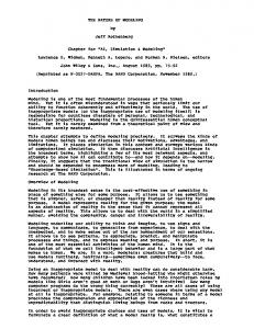
included if known. Aluminum does not have a significant strain-rate effect for velocities that occur in most aircraft crashes. For isotropic materials that are too complex to be represented with a bilinear elastic-plastic response, material models are available that allow a tabular input of engineering (or true) stress versus engineering (or true) strain. Other solid models allow volumetric crush versus strain to be input. If a tabular input is used, care must be taken to ensure that for large strains or crush, the stress is large enough to keep the element from deforming into an extremely small volume. Otherwise, the element volume can become negative (turn inside-out) and the analysis will stop executing. A large exponential “bottoming-out stress” at the end of the table may be required to prevent this behavior. A typical plot of stress versus volumetric-crush for a closed-cell foam material is shown in Figure III-1. The material response is noted to have a tensile cut-off stress, an exponential bottoming out curve, and an exponential unloading curve. In this example, the “bottoming-out” stress represents compaction of the foam material. Note that in the plot shown in Figure III-1, compressive stress is positive, and tensile stress is negative.
Stress, psi
Exponential bottoming-out curve
200 Exponential unloading curve
150 100 50
Compressive response
0 Tensile cut-off stress
-50 -100 -0.2
0
0.2
0.4
0.6
0.8
Crush Fig. III-1 – Stress versus volumetric crush for a foam material exhibiting a tensile cut-off stress, an exponential unloading curve, and a large exponential bottoming-out stress. For orthotropic and layered materials, much more work is required to define the material. For composites, a panel can be manufactured with the required lay-up, and coupons cut from the panel at 0-, 90-, and 45-degree angles. These coupons can be tested to failure in a tensile testing machine, and the results averaged to generate smeared equivalent properties. Crush tests can be performed using a special crush test apparatus [21]. Static finite element analyses of composite structures have been successful in modeling ply-by-ply composite properties with prediction of initial and progressive failure. However, this approach is not practical for analyzing failure of aircraft structure in a large nonlinear dynamic simulation. Typically, the mesh required would be too small, and the simulation time would be very large. In addition, the dynamic failure of plyby-ply composites is complicated by rate effects, delamination, and complex boundary 10
conditions. Consequently, at this time, it is often expedient to use semi-empirical data and quasiisotropic properties to model composite materials in a large crash simulation. Eulerian materials exhibit fluid behavior. Examples are water, mud, air, voids (no material), various gases, and other fluid-like materials. Since a bird is primarily water, bird strike problems are often modeled with the bird as an Eulerian material. Eulerian materials are typically modeled with an equation of state such as the gas laws where pressure is a function of volume and temperature or, equivalently, of density and internal energy. Equations of state are often written using a linear polynomial model. If one is to be successful in modeling impacts, accurate material representations must be used. In many cases, the plastic material response that occurs after yield is much more important than the original elastic material properties such as the modulus. This data is sometimes difficult to find in handbooks and often must be determined experimentally. In addition, the unloading curve is extremely important as it determines the amount of energy dissipated versus the amount of energy stored and released back into the structure. Some material models such as the FOAM2 crushable “foam” model in MSC.Dytran allows input of all of these variables. Failure It is obvious that in an aircraft crash situation, failure is observed for many components of the structure. However, severe deformation such as buckling or crushing of a finite element model does not constitute failure. Although there are algorithms that weaken an element (such as ply failure for composites), material failure in a finite element code generally means that the element is removed from the analysis. Removal of elements in a model, although often necessary, can cause the analysis to deviate from the intended path. Consequently, failure should not be allowed for initial runs of the simulation. After areas of high stress and strain are studied, and the model behavior is better understood, then failure criteria can be added to the material models. Although crack propagation could be modeled directly using nonlinear dynamic finite element codes, it is not practical for large models since extremely small elements would be required, which would adversely affect the time step by lowering it to unacceptable levels. Damping Every structure exhibits damping. For example, if a structure is struck with a hammer, the vibrations will attenuate after a few seconds and eventually stop. The damping occurs due to phenomena such as slippage in joints and fasteners, internal structural friction, visco-elastic effects, and interactions with the adjacent media, both solid supports and air. However, unless damping or failure is introduced, a finite element model of the structure will vibrate continuously. Consequently, the vibratory oscillations set up in a nonlinear dynamic finite element model are generally of high amplitude and may obscure all the underlying low frequency information that is important in the crash analysis. Finite element programs allow for damping to be applied to the whole model; however, this feature is not often incorporated except for dynamic relaxation problems. Dynamic relaxation is a technique in which the structure is first excited by an impulse and is then highly damped globally to produce a nearly steady-state solution. For example, dynamic relaxation can be used to pre-stress a panel. In addition, specific damping elements can be defined between grid points. Most contact algorithms incorporate some damping to prevent numerical instabilities.
11
Energy dissipation To correctly model material responses, both the loading and unloading curves must be carefully considered. Two interesting examples are soft soils and foams. Often experimental tabular data of stress versus strain (or crush) can be generated to characterize these materials. Although these materials may be rate sensitive, this behavior will be ignored for now. Both the loading and unloading curves need to be defined accurately for these materials. For example, objects dropped into soft sand generally exhibit no rebound velocity. This behavior can be deduced from examining the unloading curve of the sand material. The unloading curve drops to zero load almost instantaneously, with little or no energy returned (typically 99% energy dissipated). If the material is not modeled with the correct unloading curve, then elastic energy will be returned from the sand and imparted to the structure and the simulation will incorrectly exhibit a rebound velocity. Some foam models (for example FOAM2 in MSC.Dytran) allow the user to specify both the unloading curve shape and the energy dissipation factor on the material card. Various mechanisms, such as wire benders and other “energy absorbers” used to control the acceleration to an occupant in a crashworthy seat, can be modeled with either standard or userdefined nonlinear spring elements. Damping elements or global damping can also be used to dissipate energy. However, global damping is an extremely sensitive parameter and should not be used unless one understands its consequences. Also, when an element fails after meeting a preset failure criteria, the internal energy associated with that element is lost. Another energy dissipation mechanism that is nonphysical and must be watched is the energy used to control hourglassing. Hysteretic behavior Some foam materials exhibit hysteresis when they are unloaded. As mentioned above, the shape of the unloading curve (exponential, linear, cubic, etc.) and the energy dissipated can be input for some foam material models. In addition, tensile and compression load cutoff values can be input. For many of these foam models, the Poisson ratio is considered to be effectively zero, i.e, crushing the foam in one direction does not change the foam’s shape in a perpendicular direction. Initial Conditions Initial velocities, forces, etc In building a crash model, initial conditions are extremely important, especially if correlation with test data is to be performed. The initial linear and angular velocities of the aircraft, as well as the initial pitch, roll, and yaw angles must all be considered. These values are often determined from the accelerometer data and motion picture analysis. For non-zero initial attitudes, it is sometimes more convenient to rotate the simulated impact surface than to rotate the finite element model of the structure. It has been observed experimentally that an initial attitude change of less than one degree can significantly alter the crushing behavior of an object. For example, if a structure is modeled to impact perfectly flat; whereas, the actual structure impacted with a pitch of one degree, the simulation will not likely be accurate. These eccentricities are important to model as they remove symmetry from the model. In a real crash, symmetry does not exist. The structure always impacts slightly asymmetrically. Even if the structure looks perfectly symmetric on both sides of a plane of symmetry, the physical structure
12
is always weaker on one side or the other due to imperfections, manufacturing tolerances, or other factors. Initial velocities, forces, pressures, etc. can be applied to nodes as needed for a particular problem. Care must be exercised if rigid bodies are attached to non-rigid bodies as the initial velocity condition may change slightly from that input. This situation occurs due to the algorithm that initializes the velocity of nodes that are in close proximity to the rigid body. Angular velocity When initial whole-body angular velocities are required, the x, y, and z-components of the velocity vector v can be computed from the equation, v = vcg + w x r where vcg is the velocity vector of the center-of-gravity, w is the angular velocity, and r is the vector between the center-of-gravity and the point where the velocity v is to be computed. For example, the pendulum-style swing method for full-scale aircraft crash tests at the NASA Langley Impact Dynamics Research Center (IDRF) introduces a pitch angular velocity to the aircraft. Thus, in addition to the horizontal and vertical motion of the aircraft center-of-gravity, the velocity of each point away from the center-of-gravity must be recomputed taking into account the pitch angular velocity. Some codes allow for angular velocity input, but care must be taken as often the angular velocity only applies to a given rigid body. Or the angular velocity may be applied to specific nodes, not to the whole-body rotation about the center-of-gravity. Contact Definitions General Contact Nonlinear dynamic finite element codes have sophisticated contact algorithms. The contact can be defined between surfaces or between surfaces and nodes. For example, an impact surface such as the ground can be defined as a master surface and the nodes of the bottom of the aircraft can be defined as slave nodes. The master surface can also be defined as the faces of elements, either shell elements or solid elements. When a slave node penetrates the master surface, a contact force is generated that pushes the node back. A master surface has a normal vector associated with the front-side of the surface. A master contact surface may be configured to look for contact from both sides, or from only one side and to ignore nodes approaching from the other side. One error to avoid is initial contact where slave nodes have penetrated the master surface at the initiation of the simulation. A warning will be output by the code when this occurs. If the master surface and slave node contact algorithm is used, generally the master surface mesh can be very coarse. However, if the master surface is not flat, then the master surface mesh must be discretized fine enough to define the geometry of the surface correctly. There are two penalty-based methods of calculating the contact force. In the first method, the contact force on a node is based on a penetration distance times the material stiffness. In the other penalty method, the contact force is calculated using Newton’s Second Law; i.e., the contact force is proportional to the penetration distance divided by the time-step squared (average acceleration) multiplied by an effective mass. LS-DYNA primarily uses the first method, while MSC.Dytran recommends the second method.
13
Self-contact Self-contact can also be defined. An example in which self-contact should be defined is a panel that is buckling. If self-contact is not defined, shells in the panel could pass through each other as the panel forms multiple folds during compression. Friction Contact surfaces can be defined to have friction. The coefficients of kinetic and static friction can be determined experimentally, obtained from handbooks, or estimated. An example where friction may be needed is when an object impacts a slanted surface. Without friction, the object may slide down the surface before rebounding. With friction, the object will likely rebound from the surface without sliding. Contact penalty factor The default contact formulation in MSC.Dytran defines a contact force based on the penetration distance divided by the time-step squared (acceleration) multiplied by an effective mass. In the equation there is a constant known as the contact penalty factor (FACT). The default of the contact penalty factor is 0.1. There are cases when the default value must be adjusted up or down to achieve acceptable results. One case is when a very stiff or rigid material impacts a soft material. For example, consider a rigid sphere impacting soft-soil, where the sphere is the master surface and the soil nodes are slaves. When the default penalty factor is used, the soil nodes “spring away” from the spherical master surface. This behavior causes large spikes to occur in the contact force. When the default contact factor is reduced from 0.1 to 0.001, the soil nodes properly followed the leading edge of the sphere. In general, it is recommended that contact forces be output and analyzed to observe if any unusual behavior is occurring. IV. General Issues Related to Model Execution and Analytical Predictions Quality checks on model fidelity Weight and mass distribution One of the first quality checks of a model is to compare the total mass and mass distribution of the model with those of the actual vehicle or component being modeled. The mass of each material should be printed to output and compared with the expected or known mass. Center-of-gravity location Another early quality check is to compute the center-of-gravity of the model. The center-ofgravity (CG) should be compared with the center-of-gravity of the physical test article if known. For aircraft structures, the CG is often known since stability and control require the CG to lie within a given range. If the model CG is not within the operational region, then the mass distribution of the model should be modified. Misc. (modal vibration data, static load test data, etc.) Some analysts like to perform a modal analysis before running a dynamic model. This approach is particularly useful if experimental modal data is available [22]. Also, if experimental data is available for elastic loading of the structure (load-deflection data), then the model can be loaded incrementally before the dynamic analysis is performed. These quality tests are useful to verify
14
that the overall stiffness and mass distribution of the model match those of the test article. Since MSC.Nastran and MSC.Dytran inputs are basically compatible, a modal analysis of an MSC.Dytran model can be performed relatively easily in MSC.Nastran. Filtering of crash analysis data Due to the high frequency content typically seen in analytical acceleration time-histories for a particular node, acceleration data must be filtered using a low-pass digital filter. Present practice is to use a Butterworth digital low-pass filter applied forward and backward in time to avoid phase shifts in time. The choice of filter frequency is important, and engineering judgment must be used to extract the important physical information such as rise time and peak accelerations. In addition, for finite element models, the amount of mass assigned to a node can influence the choice of filter frequency. For practical purposes in test-analysis correlation, an accelerometer is used to measure acceleration at a point, which corresponds to a node in a model. Since the accelerometer plus mounting block and cable has mass, at least a small amount of concentrated mass should be placed at a node for test-analysis correlation purposes. Another approach used by some analysts is to average the response of four adjacent nodes, which acts to numerically smooth the data without using a low-pass filter. As an illustration of the effect of the filter frequency and the effect of mass applied to a node, the filtered acceleration time histories of two nodal positions on the floor of an MSC.Dytran model of a Boeing 737 fuselage section that was drop tested at 30 ft/s are plotted in Figures IV-1 through IV-3. In these figures, the acceleration responses were filtered using three different cutoff frequencies corresponding to 200-, 125- and 40-Hz, respectively. The two nodes in the model, Node 3572 and Node 3596, are located on the floor at the left inner seat track. Node 3572 is located on the front edge of the floor and has no concentrated mass associated with it. Node 3596 has 122.8-lbs. of concentrated mass assigned to it representing a portion of the seat and occupant mass. Note that the acceleration responses are extremely noisy when filtered using a 200-Hz frequency, as shown in Figure IV-1. However, the response curve for Node 3596 is much less noisy and has a lower magnitude than that of Node 3572 because it has mass associated with it. The same observation is true for the acceleration responses filtered using a 125-Hz frequency, as shown in Figure IV-2. However, when the two acceleration responses are filtered using a 40-Hz frequency, the curves are smooth and provide the underlying crash pulse at both locations, as shown in Figure IV-3. Note that many of the filtered data plots do not begin at the origin, i.e., zero acceleration at time equal 0.0-seconds. This phenomenon is an artifact of the filtering process and can be minimized to a certain extent by adding many points before the actual data having negative time and 0 or -1g acceleration, whichever value is appropriate.
15
Acceleration, g
Acceleration, g
80
80
60
60
40
40
20
20
0
0
-20
-20
-40
-40
-60 -0.05
0
0.05
0.1
0.15
0.2
-60 -0.05
0
0.05
Time, s
0.1
0.15
0.2
Time, s
Figure IV-1. 200-Hz filtered acceleration responses of Node 3572 (left) and Node 3596 (right). Acceleration, g
Acceleration, g
60
60
40
40
20
20
0
0
-20
-20
-40 -0.05
0
0.05
0.1
0.15
0.2
-40 -0.05
0
Time, s
0.05
0.1
0.15
0.2
Time, s
Figure IV-2. 125-Hz filtered acceleration responses of Node 3572 (left) and Node 3596 (right). Acceleration, g
Acceleration, g
20
20
15
15
10
10
5
5
0
0
-5 -0.05
0
0.05
0.1
0.15
0.2
-5 -0.05
0
0.05
0.1
0.15
0.2
Time, s
Time, s
Figure IV-3. 40-Hz filtered acceleration responses of Node 3572 (left plot) and Node 3596 (right plot).
16
Anomalies and errors in crash analysis data Aliasing errors Due to the high frequency content of acceleration time histories in a crash analysis, aliasing errors can occur if the time-step used for writing out the acceleration is too large. The presence of aliasing errors can be determined by integrating the acceleration time history at a node to obtain the nodal velocity. The nodal velocity obtained by integration can be compared with the velocity at the node calculated directly by the finite element program. If the two velocities do not match, aliasing errors are likely the culprit. Unfortunately, if aliasing errors are not detected, then the analytical acceleration results that are output can be misleading or completely wrong. Even writing out acceleration time histories at 10,000 samples per second, which may be the sampling rate used to collect data for a drop test, may not be adequate to avoid aliasing errors. Note that the experimental data was prefiltered so that aliasing errors will not occur. However, one cannot directly “prefilter” the analytical acceleration data at a node. It contains all of the high frequency components that are in the model. One method to effectively “prefilter” the acceleration data is to add a small amount of lumped mass to a node. This “trick” is highly recommended to avoid aliasing errors in the acceleration. Since velocity and displacement data is much smoother than acceleration data, aliasing errors are not generally a problem for these data time histories. Hour glass phenomenon Although shell elements can have multiple integration points and can be used to model bending, all of the integration points are through the center of the element. As mentioned previously, without expending any energy, adjacent shell elements can deform in-plane into nonphysical “hourglass” shapes. The model should be examined to determine if hourglassing is occurring. Algorithms have been developed called “hourglass control” that prevent this phenomena from occurring. However, if too much “hourglass energy” is used to prevent hourglassing, the solution may not be valid. Energy considerations Energy is a fundamental physical quantity. The laws of physics cannot be violated in the model, thus the total energy should not grow as the model progresses in time. The time histories of the various forms of energy, i.e., kinetic energy, strain-energy, hourglass energy, etc. should be examined individually as well as the total energy. If the model’s structural rebound height (hence velocity) is much larger than measured (from high-speed video data), then insufficient energy was dissipated by the model. This discrepancy is a common problem for models as they are often too stiff, or the unloading curves selected for the materials may not be correct. Many materials models unload along the loading curve. However, this response may not be correct and could lead to a large rebound velocity. If there is a large rebound velocity, then obviously the acceleration time history will not be correct. Either the accelerations will be too high, or the acceleration pulse will be too long. Velocity considerations Velocity is another fundamental quantity often applied as an initial condition for aircraft crash models. The initial velocity distribution should be verified, especially if one is trying to simulate rotational velocity in addition to translational velocity. The velocity time history of the structure
17
is useful as a quality check. Also, as mentioned above, if the structural rebound velocity is much larger than expected, then not enough energy was dissipated in the model. V. Experimental Data and Test-Analysis Correlation Although the focus of this paper is on crash modeling and simulation, it is equally important to address some of the issues involved in obtaining and understanding transient dynamic test data. The experimental data must be checked for quality for similar reasons that the analysis must be checked – to ensure that it is valid and as accurate as possible. The analysis cannot be verified unless the experimental data has been thoroughly checked out. Test Data Evaluation and Filtering Electrical Anomalies In addition to the actual physical data, there can be electrical noise superimposed on the experimental data. Such noise may be generated by electromagnetic interference, cross-talk between channels, inadvertent over-ranging of the instrument itself, nonlinearities caused by exciting the resonance frequency of the accelerometer, and over-ranging of the instrumentation caused by setting the voltage limits of amplifiers too low, etc. Sometimes it is difficult to distinguish between electrical anomalies and good data. Other electrical anomalies are immediately evident to an experienced researcher. During the ACAP helicopter crash test, electrical anomalies appeared in some channels. One example is a force time history plot, shown in Figure V-1, which was obtained from a lumbar load cell in an anthropomorphic dummy. Force, lbs 6000 4000 2000 0 -2000 -4000 -6000
0
0.05
0.1
0.15
0.2
0.25
0.3
Time, s Figure V-1. Electrical anomalies in dynamic load cell data.
The high peaks that exceed 6000 pounds are examples of electrical transients that are not part of the physical data. Sometimes filtering of the data will remove these electrical transients. However, filtering often does not help and can mask the anomaly making it appear as real physical data. As an example, the dummy load cell data in Fig. V-1 is filtered with a 60 Hz lowpass filter with the resulting plot shown in Fig. V-2. Note that the peak of approximately 500
18
pounds that occurs at 0.04 seconds now looks like real physical data. However, this peak load is not physical as the ACAP fuselage did not impact the concrete surface until 0.1 seconds. If an acceleration channel that has electrical anomalies is integrated, the velocity obtained will, at best, be inaccurate and could be completely corrupted. Thus, integrating acceleration data to produce velocity plots is useful for data quality checking. An example of an accelerometer data channel from the ACAP test that has electrical anomalies similar to those seen in Fig.V-1 is shown in Figure V-3. Another electrical problem is shown in Fig.V-4 where the maximum range of the amplifiers has been exceeded. Thus, the acceleration pulse has a flat-top peak that occurs around 240 g’s. While this example is fairly obvious, over-ranging can be much more subtle. When in doubt, always set up the instrumentation maximums at least a factor of two above the expected level. Accelerometers often have very high-amplitude high frequency peaks that must not overload the data acquisition system.
Force, lbs. 6000 4000 2000 0 -2000 -4000 -6000
0
0.05
0.1
0.15
0.2
0.25
0.3
Time, s Figure V-2. Lumbar load cell data filtered with 60 Hz low-pass filter.
19
Acceleration, g
Electrical Anomalies
20 10 0 -10 -20 -30 -40 -50
0
0.05
0.1
0.15
0.2
0.25
0.3
Time, s Figure V-3. Unfiltered dummy pelvis acceleration with electrical anomalies.
Acceleration, g 250 200 150 100 50 0 -50 -100
0
2
4
6
8
10
Time, ms
Figure V-4. Accelerometer data that has over-ranged the amplifiers.
20
Acceleration data Acceleration data is often difficult to interpret. An experimental structural acceleration pulse recorded from a crash test is composed of a large spectrum of frequencies superimposed together. The structure has many components, each with its own fundamental mode of oscillation, plus many harmonics. In crash dynamics, one is often concerned with the magnitude and duration of the low-frequency (fundamental) acceleration pulse that will be input into the passenger. Consequently, the high frequency ringing of the structural components is of little interest. For example, when a sled test of a seat and dummy is performed, one generally does not have to worry with the spectrum of very high frequencies as the sled has been designed to eliminate them. However, the unfiltered acceleration data from a full-scale aircraft crash contains high-amplitude high-frequency information that makes the acceleration plot difficult to interpret. Most crash data is now acquired using digital data acquisition systems. Thus, serious aliasing errors can also be introduced unless the acceleration data is pre-filtered properly before sampling. The fundamental acceleration pulse is input through the structure to the floor to the seat and into the occupant. From its definition, the average acceleration is simply the change in velocity divided by the time interval and is given by the expression: Aavg = (Vf - Vi)/(Tf - Ti) where Vf is the final velocity, Vi is the initial velocity, Tf is the final time and Ti is the initial time. The instantaneous acceleration is obtained by making the time interval very small. From calculus, the above formula implies that one can differentiate the velocity to obtain the acceleration. Conversely, one can integrate the acceleration trace to get the velocity. The initial impact velocity is known in a drop test to be the square root of twice the drop height multiplied by the acceleration of gravity (V2 = 2gh). Therefore as a quality check, AND to more accurately determine the fundamental acceleration pulse duration and rebound velocity, an integration to obtain velocity should always be performed on selected channels. If the integrated acceleration does not produce the impact velocity plus rebound, several checks must be performed. Typical questions are: was the accelerometer zeroed properly, did the acceleration trace come back to zero after impact, were the proper calibration factors used, did the accelerometer rotate or break loose in the impact, was the accelerometer hit by a flying object, was the accelerometer over ranged, was there an electrical problem? SAE filtering standards The filter used to post-process acceleration data is typically obtained from a standard such as SAE J211/1 [23]. Appendix C of SAE J211/1 presents a general algorithm that can be used to generate a low-pass Butterworth digital filter that does not shift the time phase. SAE has defined a set of Channel Frequency Classes (CFC) for impacts of vehicles, which originally were designed for automobile impacts. These CFC’s are 60, 180, 600, and 1000. However, all standards are general and cannot be applied to specific cases without detailed knowledge of their basis. From physics, the correct low-pass filtering frequency can only be determined from measuring the fundamental acceleration pulse duration. Thus, an event that occurs in a
21
millisecond should not be filtered with the same low-pass filter frequency as an event that occurs in 100 milliseconds. For extremely short duration impacts, the SAE CFC 1000 can be too low, likewise for long pulse durations the CFC of 60 can be too high to extract the underlying fundamental pulse shape. Integration as quality check By integrating the acceleration pulse, not only can a quality check of the data be obtained, but the pulse duration of the fundamental mode can also be determined. The raw acceleration data from a floor location for a 30 ft/s vertical drop test of a Boeing 737 fuselage section conducted at the FAA is shown in Figure V-5 (note that positive acceleration is up). From this plot, it is extremely difficult to determine the pulse duration. Is it 0.15 seconds, or perhaps is it 0.175 seconds? What is the peak acceleration? Based on the plot of Figure V-5, one might suggest that it is obviously about 85 g’s. However, 85-g is the absolute peak of the high frequency oscillatory response, not of the basic fundamental pulse. Also, note that the initial peak acceleration occurs in the negative direction. This behavior may seem strange at first, but it likely occurs due to a modal vibration that is set up at impact for this location. The modal vibration at time zero can be accelerating either up or down depending on the exact physical location. Acceleration, g 100 80 60 40 20 0 -20 -40 -60
0
0.05
0.1
0.15
0.2
Time, s
Figure V-5. Plot of raw acceleration data from channel 103, vertical direction. Next, the raw acceleration data shown in Fig. V-5 was integrated to produce the velocity curve shown in Figure V-6. The initial condition was applied, i.e., the velocity at time zero is –30 ft/s (downward). Unlike the complex acceleration curve shown in Figure V-5, the velocity curve in Figure V-6 is relatively simple. The velocity goes to zero at a time of 0.12 seconds, and by approximately 0.125 seconds it has gone positive to approximately 2-ft/s, which is the rebound velocity. Thus, the total velocity change including rebound is 32 ft/s. The duration of the fundamental pulse is about 0.125 seconds. Thus, the fundamental frequency is about 1/T or 8 Hz. To extract the fundamental acceleration pulse, one should use a low-pass filter that has very low attenuation at and below 8 Hz. Also, an approximation of the maximum acceleration of the
22
fundamental pulse can be obtained by simply computing the maximum slope of the velocity curve from between 0.05 and 0.1 seconds. Amax = (Vf-Vi)/(Tf-Ti) = (-5 – (-23))/(0.1 - .05) = 18 ft/s/.05 s = 340 ft/s2 Or, expressed in g-units, 11.2 g’s. Thus, without filtering, one can approximately obtain the maximum acceleration of the fundamental response of about 11.2 g’s. Velocity, ft/s 5 0 -5 -10 -15 -20 -25 -30 -35
0
0.05
0.1
0.15
0.2
Time, s
Figure V-6. Velocity obtained from integrating the raw acceleration trace in Figure V-5. The initial velocity condition (-30 ft/s) was applied as the constant of integration. Filtering to obtain fundamental acceleration pulse Next, the SAE CFC 60 low-pass digital filter is applied to the raw acceleration data and is plotted in Figure V-7. The digital filter algorithm is a 2-pole Butterworth filter. To avoid phase shifts, the filter is applied forward and then backward in time. The SAE specifies the resulting filter as a 4-pole filter. Note that the cut-off frequency for a CFC 60 is actually about 100 Hz (cut-off equals about 1.667 times CFC). Also, the formula found in Appendix C of the SAE digital filter specification states that the filter frequency equals 2.0775 times the CFC. So, the frequency input in the formula for the SAE CFC 60 low-pass filter must be 60 times 2.0775 =124.65 Hz. Since the CFC 60 digital filter algorithm is first applied forward in time and then backward in time, the cut-off frequency is reduced from 124.65 Hz on the forward pass to approximately 100 Hz on the backward pass. The CFC designations used by the SAE are somewhat confusing and are not standard filter nomenclature as used by electrical engineers; however, these standards are widely accepted for impact test analysis.
23
Acceleration, g 25 20 15 10 5 0 -5 -10 -15
0
0.05
0.1
0.15
0.2
Time, s
Figure V-7. Acceleration data filtered with SAE CFC 60 filter. The filtered response shown in Figure V-7 still contains high frequency oscillations that mask the underlying fundamental acceleration pulse. As shown in Figure V-7, the peak accelerations of the filtered data are about 25 g’s. Notice that the frequency of an adjacent maximum and minimum acceleration is about 100 Hz. If an adjacent maximum and minimum acceleration are averaged at the approximate center of the pulse (approximately 0.075 seconds), an average acceleration of (+ 17.5 g +2.5 g)/2 = 10 g’s is obtained. The 10-g value is close to the value of 11.2 g’s that was obtained earlier. Next, the original acceleration data shown in figure V-5 is filtered using a 2-pole Butterworth low-pass digital filter from 10 Hz to a maximum of 80 Hz. Since the filter is applied forward and backward in time, the corresponding cut-off frequencies are 8- and 64-Hz. The family of filtered acceleration curves is shown in Figure V-8. Each curve is labeled with the 2-pole Butterworth cut-off frequency. For example, f10 represents a 10-Hz 2-pole Butterworth filter applied twice, which effectively yields an 8-Hz cut-off frequency. Acceleration, g 20 acc, f80 acc, f60 acc, f40 acc, f20 acc, f10
15 10 5 0 -5 -10
0
0.05
0.1
Time, s
24
0.15
0.2
Figure V-8. Acceleration data filtered with 2-pole Butterworth low-pass digital filters with frequencies ranging from 10- to 80-Hz. Note that the 10- and 20-Hz filters only show one basic pulse, and that the maximum acceleration is about 12 g’s, again very close to the value calculated from the slope of the velocity curve. The rise time of the basic pulse can be used to calculate the onset rate, which is approximately 10 g/.05 sec = 200 g/second. Next, to demonstrate the effect of “over filtering” for this specific example, a low-pass filter with a frequency BELOW 10-Hz will be used. In Figure V-9, the raw acceleration data is filtered using a 5-Hz 2-pole Butterworth low-pass digital filter.
Acceleration, g's 20 15
f20 f80 f10 f5
10 5 0 -5 -10
0
0.05
0.1
0.15
0.2
Time, s Figure V-9. Acceleration data filtered with 2-pole Butterworth low-pass digital filters with frequencies of 5, 10, 20, and 80-Hz. Note that the 5 Hz filter distorts the pulse shape. The pulse shape obtained when the raw acceleration data is filtered with the 5 Hz low-pass filter is obviously distorted and spread out in time. This result confirms that the lowest filter frequency should be above 8 Hz. From Figure V-9, both the 10- and the 20-Hz filters appear to extract the fundamental pulse. However, to be conservative, the 20-Hz filter is recommended for this acceleration. The 20-Hz filter provides the least distortion at time zero, and does not spread the pulse duration. Note that the cut-off frequency for the 20-Hz digital filter is 16 Hz. Next, each of the filtered acceleration responses, shown in Figure V-9, is integrated to obtain the corresponding velocity responses, plotted in Figure V-10. The question to answer is, “Does filtering distort the velocity trace?” The velocity response obtained by integrating the 10-Hz filtered acceleration follows the velocity response obtained from the raw acceleration data quite well. Obviously, each higher low-pass filtered acceleration when integrated (such as the 20-Hz, which is recommended for this pulse) will produce a velocity curve even closer to the raw data. However, it is evident that the velocity response obtained by integrating the 5-Hz filtered acceleration distorts the original velocity data.
25
The velocity data could be integrated to obtain displacements. Even more so than with velocity, one would find that the presence or absence of the high frequency data does not influence the displacement of the test article.
Velocity, ft/s 5 0 -5 -10 vel, raw vel, f5 vel, f10
-15 -20 -25 -30 -35
0
0.05
0.1
0.15
0.2
Time, s
Figure V-10. A comparison of the velocity responses obtained from integrating the raw data, and integrating the filtered 10- and 5-Hz acceleration data. Test – Analysis Correlation It is relatively simple to evaluate test-analysis correlation qualitatively. For example, deformed structural time sequences can be compared with high-speed video frames. If the motion and structural deformation look about the same, then most authors say that they have achieved qualitative agreement. However, it is much more difficult to obtain a figure-of-merit for testanalysis correlation quantitatively. Time histories of displacement and velocity are quite useful in comparing test with analysis. The acceleration time history comparison is much more difficult to make quantitatively. The Federal Highway Administration (FHWA) has developed a set of procedures for test-analysis correlation (validation) of full-scale road vehicles in both the time and frequency domains. The National Crash Analysis Center (NCAC) at George Washington University has posted a FORTRAN program to compute some of these correlation measures. A paper by Tabiei documents the use of this procedure for obtaining quantitative validation for a simulation of a vehicle striking a guardrail [24]. Experimental and Analytical Data Evaluation - Recommended Practices Data analysis and low-pass digital filtering techniques outlined in this document to extract the basic crash pulse can be very useful when comparing seat design pulses and sled test pulses with actual aircraft crash test data. In addition, these techniques are valuable when performing testanalysis correlation. The following practices are recommended:
26
1. Always examine the raw acceleration first and look for over-ranged data, electrical drop-outs, electrical noise, and other anomalies. Document any broken or cut electrical cables, any rotated or dislodged accelerometers. Determine that the free fall acceleration is approximately -1 g, within experimental error. The acceleration should return to zero a second or two after impact. If an offset is determined, the data should be corrected. Make certain the electronic data and film or video data are synchronized so that comparisons can be made easily. 2. Integrate several of the vertical acceleration traces as a quality check to determine if the data is valid. Apply the initial velocity condition and determine if the calculated rebound velocity is reasonable when compared with motion picture or high-speed video analysis. Some rebound almost always occurs since stored elastic energy will be converted into rebound kinetic energy. Determine the total pulse duration, which is defined as the time from zero until the time of maximum rebound velocity. The duration of the pulse will determine the lowest frequency filter that should be used. Draw a straight line near the center of the velocity response to determine the fundamental pulse acceleration. The acceleration will be the slope of the straight line, which can be converted to g’s by dividing by the proper conversion factor. 3. For a test other than a vertical drop test, the acceleration pulse must be carefully examined for each orthogonal direction. 4. Filter the structural accelerometer data initially with the SAE CFC 60 low-pass filter. This filter will pass a considerable amount of high frequency ringing near 100 Hz that may mask the fundamental pulse. Seated occupants in a typical survivable crash do not respond to the high frequency ringing. Use the pulse duration obtained in step two to develop a low-pass filter to extract the fundamental crash pulse. For many cases, a 20-Hz low-pass filter will produce good results. 5. For analytical results, recognize that the amount of mass applied to a node in a finite element model can greatly influence the amplitude of high frequency ringing in the acceleration response. One method of reducing the oscillatory response of a node is to apply a small concentrated mass to the node. Another method is to average the acceleration responses of two adjacent nodes that are reasonably close together. Be careful to extract time history data at sufficiently high frequency so that aliasing errors do not occur. 6. When performing test and analysis correlation, it is often useful to first examine velocity and displacement data. Displacement data can be measured as time-history graphs, or overall displacement data such as motion picture data can be compared with computer graphics plots at the same time. Both acceleration data from the test and nodal acceleration from the model must be filtered before they can be compared. However, it is not sufficient to sample both the experimental data and the nodal data say at the same rate and then filter with the same low pass filter. Note that the experimental data was pre-filtered before sampling. Also note that the model’s high-frequency amplitudes are undamped and thus much higher than the comparable test data.
27
VI. Conclusions Recent advances in computer software and hardware have made possible analysis of complex nonlinear transient-dynamic events that were nearly impossible to perform just a few years ago. Unlike automotive impact testing, which is now a routine part of the development process, crash testing of even small aircraft is rarely performed due to the high cost of the aircraft and the myriad of crash impact conditions that must be considered. Crash simulations are currently used as an aid in designing, testing, and certifying aircraft components such as seats to dynamic impact criteria. Ultimately, a primary goal to enhance aviation safety is to utilize full-scale crash simulations of the entire aircraft for design evaluation and certification. The objective of this paper is to document “best practices” for performing aircraft crash simulations using commercially available, explicit nonlinear dynamic finite element codes. Although “best practices” is somewhat relative, the authors’ intent is to help others to avoid some of the common pitfalls in impact modeling that are not generally documented. T h e learning curve is quite steep in moving from a linear static structural finite element code to a nonlinear transient dynamic finite element code. In addition, many assumptions and simplifications are often made by the developers to make the code run efficiently. The user needs to have a basic understanding of the underlying assumptions and limitations of the elements and algorithms in the nonlinear dynamic code to be successful in crash modeling. Even after the model has successfully executed without runtime errors, quality checks of the results for “sanity” and for energy growth must be performed. In addition to providing information on building, executing, and validating models, a discussion of experimental data analysis, filtering, and test-analysis correlation is included. This information provides insight to help evaluate the validity and accuracy of experimental crash data. Quality checks such as integrating the experimental acceleration to determine if the resulting velocity is physically meaningful are important to the crash analyst. Experimental data with electrical anomalies must be carefully filtered to avoid masking the anomaly and making it appear as real physical data. Once confidence in the experimental data is achieved through the quality checks outlined, then a test-analysis correlation can be considered. Finally, some examples of aircraft crash models are described in detail in the appendices with comments on the modeling approach and with “lessons learned.” These examples cover both composite and conventional aluminum aircraft structures. VII. References 1. Gamon, M., Wittlin, G., and LaBarge, B., "KRASH 85 User's Guide- Input/Output Format,” Final Report DOT/FAA/CT-85/10, May 1985. 2. Walton, Andrew, Whayeb, Shakir, and Sadeghi, Majid, The Air Accident Investigation Tool, Second International KRASH User’s Seminar, Cranfield Impact Centre Ltd, England, 26028 June 1995. 3. LS-DYNA User’s Manual, Livermore Software Technology Company, Livermore, CA, 1997.
28
4. Hallquist, J. O. and Whirley, R. G., DYNA3D User’s Manual. UCID-19592, Rev. 5, Lawrence Livermore National Laboratory, May 1989. 5. MSC.Dytran User’s Manual Version 4.7, Volumes 1 and 2. MSC Software Corporation, Los Angeles, CA, 1999. 6. Lahey, R. S., Miller, M. P., and Reymond, M., MSC/NASTRAN Reference Manual, Version 68, MSC.Corporation, 1994. 7. Pifko, A., Armen, Jr., H, Levy, A., and Levine, H., PLANS – A Finite Element Program for Nonlinear Analysis of structures, Volume II – User’s Manual. NASA CR-145244, 1977. 8. Pifko, A. B., Winter, R., and Ogilvie, P. L., DYCAST - A Finite Element Program for the Crash Analysis of Structures. NASA CR 4040, January 1987. 9. Hallquist, J. O., NIKE3D: An implicit finite-deformation, finite element code for analyzing the static and dynamic response of three-dimensional solids. Lawrence Livermore National Laboratory, UCID-18822, Rev.1, July 1984. 10. PAM-CRASH, Engineering Systems International SA, F-94588 Rungis, France. 11. Fasanella, E. L., Boitnott, R. L., Lyle, K. H., and Jackson, K. E., Full-scale crash test and simulation of a composite helicopter, International Journal of Crashworthiness, Vol. 6, No. 4, November 2001, pp. 485-498. 12. Stockwell, Alan E., Evaluation of Modeling and Simulation Tools and Techniques for an Analytical Study of the Lear Fan Impact Test, NASA CR-2002-211457, March 2002. 13. Dynamic Analysis and Design System Revision 9.0 Reference Manual. Computer Aided Design Software, Inc., Coralville, IA, 1998. 14. Fasanella, E. L., Lyle, K. H., Pritchard, J. I., and Stockwell, A. E., Simulation of X-38 Landing Scenarios with Landing Gear Failures. NASA TM-2000-210078, March 2000. 15 MADYMO Users’ Manual 3-D Version 4.3, the Dutch Institute of Applied Scientific Research – Road/Vehicles Research Institute, Department of Injury Prevention, October 1988 16. Obergefell, L. A., Gardner, T. R., Kaleps, I., and Fleck, J. T., Articulated Total Body Model Enhancements, Volume 2: User's Guide. AAMRL-TR-88-043, January 1988. 17. Fasanella, Edwin L. and Jackson, Karen E., Impact Testing and Simulation of a Crashworthy Composite Fuselage Section with Energy-Absorbing Seats and Dummies, 58th AHS Annual Forum, Montreal, Canada, June 11-13, 2002.
29
18. Brinkley, J. W., and Shaffer, J. T., "Dynamic Simulation Techniques for the Design of Escape Systems: Current Applications and Future Air Force Requirements," Aerospace Medical Research Laboratory; AMRL Technical Report 71-292, Wright-Patterson Air Force Base, Ohio, December 1971, AD 740439. 19. MSC/PISCES-2DELK User’s Manual, The MacNeal-Schwendler Corporation. 20. Pentecote, N. and Vigliotti, A., Simulation of the Impact on Water of a Sub-Floor Component and Full-Scale WG30 Helicopter, 58th AHS Annual Forum, Montreal, Canada, June 11-13, 2002. 21. Lavoie, J. A., Morton, J., and Jackson, K. E., An Evaluation of the Energy Absorption of Laminated Composite Plates, Journal of Aerospace Engineering, Proc., ImechE, Vol. 209 (G3), September, 1995, pp. 185-194. 22. Lyle, K. H., Bark, L. W., and Jackson, K. E., “Evaluation of Test/Analysis Correlation Methods for Crash Applications.” Proceedings of the American Helicopter Forum 57, Washington, D.C., May 9-11, 2001. 23. Society of Automotive Engineers, Recommended Practice: Instrumentation for Impact Test – Part 1, Electronic Instrumentation, SAE J211/1, March 1995. 24. Tabiei, Ala and Wu, Jin, Validated crash simulation of the most common guardrail system in the USA. International Journal of Crashworthiness 2000, Vol5, No.2, pp. 153-168
30
APPENDIX A. SIKORSKY ACAP HELICOPTER CRASH SIMULATION A.1 Experimental Program A.1.1 Test set-up In 1999, a full-scale crash test of the Sikorsky Advanced Composite Airframe Program (ACAP) helicopter, shown in Figure A-1, was performed at the Impact Dynamics Research Facility (IDRF) that is located at NASA Langley Research Center in Hampton, VA [1]. The helicopter was the flight test article built by Sikorsky Aircraft Corporation under sponsorship by the U.S. Army during the Advanced Composite Airframe Program [2-5]. The primary objective of the crash test was to provide experimental data for validation of an explicit, transient dynamic finite element crash simulation. The general configuration of the ACAP airframe is derived from Sikorsky's S-76 commercial aircraft. The dynamic components of the ACAP helicopter, such as the rotor blades, rotor transmission, and engines are the same as those used on the S-76. However, the airframe and landing gear were completely new designs. Crashworthy design features of the helicopter include the main and nose landing gear, the airframe and energy absorbing subfloor, the crew and troop seats, and the fuel system. A complete description of these energy-absorbing features can be found in Reference 3.
Figure A-1. Photograph of the Sikorsky ACAP test article. Several modifications were made to the helicopter in response to information acquired from a previous crash test of the Sikorsky ACAP static test article in 1987 [3] to improve the energy absorbing capabilities of retrofit equipment. For example, the original energy absorbing nose gear was missing from the helicopter and had been replaced with a non-crashworthy civil helicopter gear. Modifications were made to increase the energy absorption capabilities of the nose gear. However, even with the modifications, the retrofitted nose gear could only absorb a small percentage of the energy that the original gear was designed to remove. One of the main energy absorbing devices for the structure was the crushable lower portion of the keel beams and subfloor bulkheads. There were four keel beams beneath the floor, two inner keel beams and two outer keel beams. The keel beams and transverse bulkheads beneath the floor were constructed of two horizontal C-channels, one above the other, with a beaded (or waffle) web geometry. The upper channel was constructed of graphite and the lower 4-inch high beaded web was constructed of Kevlar. The lower portion of the inner keel and bulkhead beams
31
was fabricated of a thinner beaded Kevlar construction designed to crush and absorb energy. The graphite upper channel was not intended to crush, and was designed to support the floor and to react the crushing loads from the lower Kevlar channel. A photograph of the subfloor design is shown in Figure A-2 (a) and a schematic drawing of the lower forward fuselage is shown in Figure A-2 (b), in which the crushable lower portion of the subfloor is illustrated by the crosshatched area.
(a) Photograph of the subfloor consisting of two horizontal C-channels, one above the other with a beaded (or waffle) web geometry. Controls closet Windshield center post
FS 143
Crush zone
Nose gear trunnion support
FS 188
FS 122
Fuselage skin
Crushable zone
Outboard keel beams
Inboard keel beams Canted rib
(b) Schematic drawing of the lower forward fuselage. Figure A-2. Details of the lower forward fuselage. For the test, the aircraft was outfitted with two crew and two troop seats, and four anthropomorphic test dummies. The seats and dummies were instrumented with accelerometers and loads cells to measure the occupant responses during the crash test. The helicopter was instrumented with accelerometers located on the airframe, the main and nose landing gear, and
32
large mass items such as the rotor transmission and engines. In total, 110 channels of data were transmitted through an 800-ft.-long umbilical cable (data transfer wire) for collection. The helicopter was suspended from the IDRF overhead gantry and crash tested by swinging it pendulum-style into a concrete impact surface. A general diagram of the crash test method is given in Figure A-3. The intended vertical and horizontal impact velocities were 38- and 32.5fps, respectively. The intended impact orientation was 5° nose-up pitch with no roll or yaw. Additional information on the ACAP helicopter crash test procedure can be found in Reference 6. General full-scale crash test procedures are described in Reference 1.
Figure A-3. IDRF gantry structure used to perform crash test of the ACAP helicopter. A.1.2 Summary of Test Results A summary of the test results obtained during the crash test of the Sikorsky ACAP helicopter is provided in this section of the paper. Additional information regarding the 1999 full-scale crash test can be found in Reference 7. A post-test photograph is shown in Figure A-4. The actual measured impact conditions were 38-ft/s vertical and 32.5-fps horizontal velocity with 6.25° nose-up pitch, and 3.5° left-down roll. In addition, the pendulum-style swing method that was used in conducting the ACAP helicopter crash test introduced a pitch angular velocity to the airframe. The magnitude of the pitch angular velocity was determined from high-speed motion analysis to be 9.6°/second (increasing nose-up). Test data and the high-speed films were used to determine the time sequence of events. The reference time (0.0 seconds) was defined as the time of initial contact of the left main gear tire. The right gear tire impacted the ground .012 seconds after the left gear tire impacted, and the nose gear impacted at .069 seconds. The fuselage section did not contact the ground until 0.098 seconds. The helicopter modifications made in response to information acquired from the 1987 crash test were successful. During the impact test, the nose gear stoked 9 inches. However, the retrofitted nose gear was not designed to withstand a high velocity impact and failed early providing little energy absorption. The left and right main landing gear stroked 13.2 and 11.8 inches,
33
respectively. No failures of the landing gear attachments occurred. Separation and failure of the tail cone initiated while the landing gear was stroking. The floor level vertical accelerations were approximately 85 g’s with the accelerations slightly higher towards the front of the helicopter due to slap down. The peak accelerations were lower towards the top of the helicopter. The seat pan accelerations were lower than the floor-level accelerations, but were still too high to avoid injury. The copilot crew seat bottomed out because of the absence of the original high capacity, energy absorbing nose gear.
Figure A-4. Post-test photograph of the ACAP helicopter in its final resting position. A.2 Description of the Modeling Approach A limited number of structural and/or engineering drawings were available for use in development of the geometry model of the Sikosky ACAP helicopter. Consequently, a photogrammetric survey was conducted of the outer surface of the helicopter. A photograph of the helicopter during the survey in shown in Figure A-5 and the resulting points defining the outer surface of the helicopter are shown in Figure A-6. The plans were to use the point coordinates to create curves and surfaces defining the outer skin of the fuselage section. Then, hand measurements would be used to define the geometry of the interior structure. The geometry model would be discretized and meshed to create the finite element model. However, before this process could begin, an existing MSC.Nastran [8] modal vibration model of the Sikosky ACAP helicopter was obtained. The MSC.Nastran model of the ACAP helicopter that was originally developed for correlation with modal-vibration data was obtained from Sikorsky Aircraft Corporation [9]. The model, shown in Figure A-7, had approximately 5000 nodes, 9,500 elements, 220 material models including many different composite materials, and over 700 different property cards. The elements included 5,453 shell elements; 1,956 beam elements; 1,770 rod elements; and 372 concentrated masses. Because this model was originally used for modal analysis, extensive modifications were required to convert it for a crash simulation.
34
Figure A-5. Photograph of the ACAP helicopter during the photogrammetric survey.
Figure A-6. Coordinate points obtained from the photogrammetric survey.
Figure A-7. MSC.Nastran modal-vibration model of the ACAP helicopter. The initial work in converting the modal-vibration model to an input deck suitable for crash simulation concentrated on combining elements, deleting unnecessary elements, and rediscretizing the model. The original linear elastic material property cards had to be modified to
35
include yield stress, strain hardening, density, and maximum strain to failure, as appropriate. The finite element mesh of the tail cone was greatly simplified, and the elements representing the stabilizer and rudder were removed. A transition mesh was developed to connect the coarse mesh of the tail cone to the finer mesh of the fuselage cabin. Many of the original triangular elements were combined and converted to quadrilateral elements. Triangular elements are not recommended for models that undergo large deformations as they are typically too stiff. In the original Nastran model, all structural inertia was input using concentrated mass and no material densities were defined. Consequently, in converting the model for crash simulation most of the original concentrated masses in the modal-vibration model were removed. Other concentrated masses were modified or added to represent actual lumped masses on the helicopter including the rotorcraft transmission, engines, anthropomorphic dummies, seats, fuel, instrumentation boxes, batteries, and cameras, etc. The elements in the original modal-vibration model representing the main and nose landing gear were removed. An external user-written subroutine was developed to calculate the main landing gear forces as a function of velocity and stroking distance including both the oleo-pneumatic and the crushable honeycomb stages. The original crashworthy nose gear of the ACAP helicopter had been removed and replaced with a non-crashworthy standard nose gear. Modifications were required to make the existing nose gear more crashworthy. The hydraulic fluid was drained, and a thin-walled aluminum tube with a honeycomb core was inserted inside the gear to provide some energy absorption. The modified nose gear was modeled as a spring having a constant spring force of 8,000-lb. to represent the crush strength of the honeycomb-filled aluminum tube. Since the original modal-vibration model was too detailed in some regions and too coarse in other regions, some rediscretization of the mesh was made. One of the main energy absorbing devices for the structure was the crushable lower portion of the keel beams and subfloor bulkheads. There were four keel beams beneath the floor, two inner keel beams and two outer keel beams. The keel beams and transverse bulkheads beneath the floor were constructed of two horizontal C-channels, one above the other, with a beaded (or waffle) web geometry. The upper channel was constructed of graphite and the lower 4-inch high beaded web was constructed of Kevlar. The outer keel beams were very thick and did not crush in the test. The lower portion of the inner keel and bulkhead beams was fabricated of a thinner beaded Kevlar construction designed to crush and absorb energy. In the original modal-vibration model, the crushable Kevlar web was modeled using 4-inch-high shell elements with longitudinal beam elements to represent the flanges of the C-sections. The Kevlar shell elements representing the keel beam and the bulkheads were rediscretized by dividing each original shell element vertically into four shell elements. This representation, as shown in Figure A-8, allowed crushing to occur. Following the extensive modifications, the ACAP helicopter crash model executed with a time step of approximately 1.9 microseconds. The model was run many times to track down the elements controlling the time step. These elements were then combined with other elements to increase the time step to an appropriate duration to allow a reasonable run time for the model. The MSC.Patran pre- and post-processing code was used with the MSC.Dytran “Preference” to build and modify the finite element crash model and to post-process the results [10].
36
Figure A-8. Finite element model of the subfloor of the ACAP helicopter. The final crash model of the ACAP helicopter is shown in Figure A-9. The model consists of 4,128 grid points and 7,346 elements, which include 3,118 beam and rod elements, 3,283 quadrilateral shell elements, 695 triangular shell elements, and 250 solid elements that represent the impact surface. The number of different material property cards was reduced from 219 in the MSC.Nastran modal-vibration model to 34 in the MSC.Dytran crash model. In addition, the number of different property cards for shell elements was significantly reduced by combining many of the PCOMP cards. The PCOMP cards are used in MSC.Dytran to specify the material properties and orientations of each ply in a laminated composite shell element. (Please note that words that appear italicized and in all caps refer to specific cards used in the MSC.Dytran input deck.) Also, the total number of concentrated masses in the model was reduced from 372 in the modal-vibration model to 98 in the crash model. The 98 concentrated masses represent actual lumped masses used in the experiment. In the final crash model, the structural elements weighed 2,838-lb. and the concentrated masses weighed 5,160-lb., for a total weight of 7,998-lb. The actual test article weighed 7,832 lbs. A flat plate consisting of 250 solid elements with fixed bottom nodes was added to the model to represent the impact surface. A master surface to slave node contact was defined between the flat impact surface and the nodes in the structural model. The initial conditions including the pitch and roll angle and the translational and rotational velocities were determined from measurements made from the high-speed video and from motion picture analysis of the highspeed film. The coordinate system used in the model was x-axis positive from nose to tail, z-axis positive up, and y-axis position to the right. The nominal impact conditions are -38.5 fps vertical velocity, -32 fps longitudinal velocity, 9.6°/second pitch angular velocity (rotating nose up and tail down due to swing), 6.25° nose-up pitch, and 3.5° left-down roll. For this simulation, it was more expedient to adjust the position of the impact surface, rather than the structural model to account for the roll and pitch attitude. The positions of the center-of gravity for the helicopter
37
model were determined to be FS = 203.7-in., BL = 0-in., and WL = 87-in. Note that these dimensions are given in reference to the manufacturer’s Fuselage Station (FS), Butt-Line (BL), and Water Line (WL) coordinate system. In comparison, the measured location of the center-ofgravity of the test article was FS = 198-in., BL = 0-in., and WL = 100-in. Note that the WL location of the center-of-gravity is difficult to determine experimentally and the measured value may not be highly accurate.
z y x
(a) Side view.
(b) Three-quarter view. Figure A-9. Final crash model of the ACAP helicopter. To perform the simulation, a two stage modeling approach was employed in which a rigid structural model of the helicopter was executed during deformation of the landing gear. At 0.045 seconds before fuselage contact, the x, y, and z- locations of all grid points and the corresponding nodal velocities in the rigid model were output to a file. These initial conditions were then input as the starting point of the flexible model simulation. The rigid-to-flexible approach was used to significantly decrease the CPU time required to complete the simulation, and because the rigid model made the introduction of the pitch angular velocity easier. The development of the landing gear model, rigid structural model, and flexible structural model are discussed in the following subsections.
38
A.2.1 Landing gear model For impacts on hard surfaces, accurate simulation of the energy absorbing response of the landing gear is imperative to accurately predict the impact response of the fuselage. The landing gear stroking not only reduces the fuselage impact speed, but can also change the impact attitude. The stroking of the landing gear, which can typically last 0.1 seconds, generally provides low acceleration levels and primarily elastic deformations to the fuselage, as compared to the fuselage impact event. These facts enabled utilization of a rigid fuselage model during most of the landing gear stroking. The time step for a rigid model is typically an order of magnitude larger than that for the flexible model, therefore the required clock time to perform a simulation is reduced by an order of magnitude. For the model presented here, the CPU time was reduced by a factor of eight. Additional details regarding the landing gear modeling can be found in Reference 11. A schematic of the ACAP main landing gear as viewed aft of the aircraft is shown in Figure A10. The main gear were designed with a two-stage, energy absorption approach. For landings within the normal operational range, an oleo-pneumatic energy absorber was incorporated. For severe or crash landings, additional energy is absorbed through stable crushing of an aluminum honeycomb column within the gear. The transfer from the oleo-pneumatic to the honeycomb stage is accomplished by shear pin failures based on a predetermined force. The orientation of the gear with respect to the fuselage remains nearly constant while the oleo-pneumatic stage is stroking. The initial angle with respect to the vertical, as shown in the figure, is 11.8 degrees. As the honeycomb crushes, the gear rotates outward an additional 20 degrees. The drag beam controls the gear rotation. Vertical
Honeycomb tube Fuselage attachments
20.0o Fully-compressed position
Oleo-pneumatic
Drag beam
Fully-extended position
11.8o
Figure A-10. Schematic of ACAP landing gear looking aft. To simplify the finite element model of the main landing gear mechanism as much as possible, the angle of the landing gear was fixed with respect to the aircraft vertical axis. Therefore, the
39
translational and rotational motions of the gear have been replaced with purely translation motion. The angle was determined by bisecting the angle through which the gear strokes, or 11.8o + 0.5 x 20o = 21.8o, as shown in Figure A-10. Initially, the landing gear model was to be developed using a number of rigid joints, such as sliding, rotational, ball, and universal joints that are currently available as standard capabilities in commercial codes. However, these joints may become unstable when large forces are applied such as those experienced by the landing gear during a severe impact. For this reason, these built-in joints were replaced in the model with a component containing a single spring element with a user-defined force response to represent both the oleo-pneumatic and crushable honeycomb stages, and several beam elements that were used to define the correct gear geometry and to distribute the constraint forces, as shown in Figure A-11 (a). In general, the “spring” force equation can be dependent on the relative displacement and the relative velocity of the connected nodes. This flexibility allows a user-defined spring to simulate the response of the velocity dependent oleo-pneumatic stage and the crushable honeycomb stage, which depends only on displacement. A FORTRAN subroutine was written to simulate the force applied to the fuselage by the main landing gear as they stroke. The equations defining the oleo-pneumatic portion are found in the KRASH 85 User’s Guide: Appendix A [12]. The equations account for the air spring friction, hydraulic damping and coulomb friction. The values for the various parameters defining the ACAP main landing gear were taken from information supplied by the airframe manufacturer. The transition from oleo-pneumatic to honeycomb crushing results from the shear pin failures in the test article. Because the oleo-pneumatic friction forces are dependent on the velocity, an extremely large, short duration force is applied at the initiation of contact. For this reason, the simulation was not able to use the computed force to determine the transition. As an alternative, the displacement (stroke) of the oleo-pneumatic portion was used to trigger the transition. The crushing of the honeycomb stage is represented by a constant force of 28,000 lb. After fuselage contact, the force due to the landing gear is reduced to zero as an approximation of the transfer of the load from the gear to the fuselage belly. Alignment of the landing gear model relative to the aircraft can be a challenging modeling problem. For this simulation, nodal alignment was accomplished by creating four contact surfaces on the outer surface of two perpendicular plates. Each perpendicular plate was modeled with a rigid quadrilateral shell element. The nodes of the spring and beam elements forming the landing gear model were then constrained to remain within the intersecting region of the perpendicular shells, as illustrated in Figure A-11 (b). The thickness of the alignment shells was set to provide sufficient stability without creating extremely large contact forces. For the results presented in this paper, the shell thickness was 0.010 in.
40
View A-A
Fuselage attachment
Spring Spring element
Alignment area
Beam elements with associated nodes
Beam elements 21.8o
Shell thickness = 0.01 inch (exaggerated)
Tire
Perpendicular surfaces (a) Aft view, not to scale. (b) View A-A, not to scale.
Figure A-11. Schematic of landing gear in the finite element model. The original crashworthy nose gear was missing and had been replaced with a non-crashworthy standard nose gear. As described previously, modifications were required to make the existing nose gear more crashworthy. The retrofitted nose gear was modeled as a spring having a constant spring force of 8,000 lb. to represent the crush strength of the honeycomb-filled aluminum tube that was inserted inside the gear. A.2.2 Rigid structural model A rigid structural model of the ACAP helicopter was created by changing all of the material properties assigned to the elements to MATRIG, except for those elements forming the landing gear. MATRIG is a specific material property card in MSC.Dytran that allows elements to be defined as rigid bodies whose mass and moments of inertia are determined by the element geometry and defined density. Once MATRIG is defined for an element, it cannot deform and the code simply tracks the kinematic motion of the element as the simulation progresses. As described in the previous section, landing gear forces were computed using an external subroutine. This procedure allowed quick runs to be made, of approximately one-hour duration, to refine the correlation of the sequence of events, and to ensure that the landing gear subroutine accurately predicted the gear forces. For this model, it was important to ensure that the location of the center-of-gravity and moments of inertia matched the experimental values closely. The rigid model was executed for a duration of 0.045 seconds after left gear tire contact. The archive files generated by the rigid model were post-processed in MSC.Patran with user-written commands to create files containing nodal velocities and nodal positions at 0.045 seconds. The nodal position file, which had the new GRID locations for each node, was input into the flexible model using the INCLUDE statement. The velocity file was read into the flexible model by an external user-written FORTRAN subroutine.
41
The choice of 0.045 seconds as the transition time between the rigid and flexible simulations was made for several reasons. Ideally, the optimal approach would be to run the rigid simulation up to 0.097 seconds, or just prior to fuselage contact with the ground which occurred at 0.098 seconds. Then the transition to a flexible model would be performed to capture the fuselage deformations after that time. This approach would have been used had the fuselage exhibited only rigid body motion from the time of left tire contact to fuselage contact. However, deformation of the tail cone initiated immediately following impact and separation of the tail cone from the main fuselage was visible at 0.064 seconds. Thus, it was necessary to adjust the transition time to better capture the tail cone response. Also, the shear pin failure in the right main landing gear occurred at 0.045 seconds, at which point the landing gear response was modeled with a constant spring force representing the crushing of the honeycomb stage. A.2.3 Flexible structural model The flexible structural model was the same as the rigid model except for the following modifications. The material cards were non-rigid, the initial GRID coordinates were the nodal positions of the rigid model at 0.045 seconds, and the initial velocity of each node was read in by the user subroutine from the rigid model at 0.045 seconds. Also, during this latter stage of the analysis, each landing gear force was modeled using the appropriate constant honeycomb crushing force, 8,000 pounds for the nose gear and 28,000 pounds for the right and left main gear. The transition occurred without incident except for a slight discontinuity that occurred when the flexible model was initiated. The flexible model included the effects of gravity, however friction of the impact surface was not included. Friction is difficult to measure experimentally, and would only be significant after fuselage contact. Since friction was not modeled, no results are shown for the longitudinal (forward) or lateral (side) directions. To run the flexible model for 0.1 seconds real time (from 0.045 to 0.145 seconds) required approximately 12 CPU hours on a Sun Ultra Enterprise 450. The flexible model is computationally intense compared with the rigid model, which required approximately 30 minutes to run a .045 second simulation. Note that current workstation computers are much more efficient and the simulation time for a model such as this would be expected to decrease significantly. Additional information regarding the development of the crash model and the modeling approach may be found in References 13-15. A.3 Lessons Learned The modeling effort described herein is one of the first complete explicit finite element crash simulations of an impact test of a composite helicopter including energy absorbing main and nose landing gear. In addition to these highly complex structures, the model attempted to capture all of the initial conditions including impact velocity and pitch rate, as well as the pitch and roll impact attitude. However, several simplifying assumptions were required. Even though an induced pitch angular velocity was determined, any roll or yaw rate was assumed to be zero. Also, the landing gear mechanism was complex and for simplicity required several approximations to be made that eliminated the sideward motion of the gear as it stroked. The rigid-to-flexible two-stage modeling approach was implemented as the most efficient means of simulating the landing gear response. In addition, the transition between rigid to flexible models
42
caused a slight discontinuity that occurred when the flexible model was initiated due to the instantaneous onset of the full landing gear honeycomb force. Several techniques to minimize discontinuities (e.g., an acceleration spike at the transition point from the rigid to flexible models) were investigated, such as ramping the honeycomb force over multiple time steps. However, none of these approaches was completely effective. The rigid-to-flexible two-stage modeling approach, along with the other simplifications, did introduce some inaccuracies into the model. For example, during the crash test, the tail deforms and begins to fail soon after the landing gear forces are applied and before fuselage contact with the ground. However, in the current modeling approach, the fuselage tail was represented as a rigid body for the first 0.045 seconds of the simulation. Consequently, the simulation did not predict the deformation of the tail from initial contact to 0.045 seconds. The rigid-to-flexible modeling approach was used because it offered an efficient means of introducing the pitch angular velocity. Another approach to account for the angular velocity would have been to write an external subroutine to calculate the initial x, y, and z components of velocity in the global axis system for each node in the model. When first comparing analytical and experimental data, it is often difficult to use the raw, or even the filtered, acceleration responses to understand the physics of the impact event. In most cases, it is better to examine and compare the velocity responses. Kinetic energy is proportional to velocity squared, hence inaccuracies in velocity are quite important. Since the helicopter had a pitch rate about the center-of-gravity induced by the pendulum-swing test method, each longitudinal point on the helicopter had a different vertical and horizontal component of velocity. Any inaccuracy in the landing gear forces, landing gear mechanism, and in the landing gear and tire friction (which was ignored) during the rigid body phase causes not only the center-ofgravity velocity to be incorrect, but also the rotational velocity about the center-of-gravity to vary incorrectly. To illustrate the velocity comparisons, the predicted and experimental velocities at 0.045- and 0.095-seconds and the percentage difference between them are provided in Table A-1 for nine different locations on the airframe. These times were chosen for their significance in the simulation and in the time sequence of events. The time of 0.045-seconds was chosen because it is the transition time between the rigid and flexible simulations and the time of 0.095 seconds was chosen because it is just prior to fuselage contact with the ground. The percentage differences listed in Table A-1 were obtained by subtracting the experimental value from the analytical value, then the difference was normalized by the experimental value. Thus, a positive percent difference represents an under prediction of the data, while a negative value represents an over prediction. The velocity responses from the rigid simulation at 0.045 seconds agree extremely well with the experimental values, within ±5%. However, by the time of fuselage contact, some deviations have occurred, most notably for the right and left engine locations. Normally, one would consider that these errors are a result of inaccuracies in the model; however, in this case, the differences are due to electrical anomalies in the test data that adversely influenced the integrated velocity responses. The floor-level velocity responses for the crew and troop seat locations and at FS 182 agree well with the test data at both .045- and .095-seconds. The accuracy of the
43
predicted floor-level responses is more important than at other locations, since the floor-level acceleration pulse is transmitted through the seats to the occupants. Table A-1. Comparisons of predicted and experimental velocities for time = 0.045- and 0.095seconds at nine locations. Location
Velocity (in/s) at time Velocity (in/s) at time = = 0.045 s 0.095 s Test Analysis % Diff Test Analysis % Diff Pilot seat floor -447.1 -456.4 -2.0 -483 -470.2 2.7 Copilot seat floor -444.4 -436.3 1.8 -452.6 -458.5 -1.3 Top rt. main gear -403.5 -382.5 5.2 -232.5 -181.3 22 Right engine -362.6 -361.4 .3 -158.2 -209.4 -32.4* Left engine -353.8 -361.3 -2.1 -155 -201.4 -29.9* Right troop floor -415.8 -411.9 .9 -312.3 -319.3 -2.2 Left troop floor -405.3 -403.2 .5 -299.7 -311.4 -3.9 Rotor head -393.6 -393.1 .1 -271.1 -262.3 3.2 Floor at FS 182 -412.3 -399.6 3.1 -311.4 -277.8 10.8 * Electrical anomalies in the acceleration responses caused errors in the integrated test velocity responses. A similar comparison of predicted and experimental peak acceleration values was made for the same nine locations as shown in Table A-2. Note that the experimental peak acceleration values were used to normalize the differences. The data shown in Table A-2 do not reflect differences in phasing, i.e., time of occurrence of the peak acceleration values. Also, the data were obtained from the plots of filtered analytical and experimental data. The same low-pass digital filter was used for both sets of data. As shown in Table A-2, the predicted peak acceleration values of five of the nine locations are within 20% of the experimental data. All of the predicted values are within ±40% of the experimental data with the exception of the rotor head location. The large over prediction in the peak acceleration of the rotor head may be attributed to two factors. First, a large number of vertical rod elements were used in the original modal-vibration model. During the conversion of the modal-vibration model, all of the rod elements in the subfloor were either removed or replaced with beam elements, since rod elements cannot bend and are thus too stiff to represent the actual structural crash behavior. However, not all of the rod elements in the upper fuselage were removed. Thus, the model of the upper fuselage had a higher stiffness and exhibited less deformation than the actual structure, which contributed to the over prediction of the peak acceleration. Another factor that may have contributed to the large difference in peak acceleration at the rotor head location is the fact that the mass and inertia of the troop seats and occupants were represented as concentrated masses that were attached to nodes on the floor in the rear cabin area. However, the troop seats were mounted directly to the ceiling, just under the rotor head location. A large downward deflection of the helicopter's roof at the location of the wire-bender suspension system was observed in the high-speed film coverage. Since the mass of the troop seats and occupants were not accurately located in the model, this load path was not represented.
44
Table A-2. Comparisons of predicted and experimental peak accelerations at nine locations. Location Pilot seat floor Copilot seat floor Right main gear (top) Right engine Left engine Right troop floor Left troop floor Rotor head Floor at FS 182
Test 90.1 82.8 33.8 42.8 40.9 75.4 85.6 27.4 61.1
Peak acceleration, g Analysis % Diff 115.6 -28.4 114.9 -38.8 33.2 1.6 34.7 18.9 40.7 .5 63.6 15.7 51.7 39.6 47.1 -71.8 53.7 12.1
The results in Table A-2 appear to raise questions regarding the accuracy of the correlation between the crash simulation predictions and the test data. However, several factors must be considered in the evaluation of this data. Correlation between analytical predictions generated from a crash simulation and transient dynamic test data is not straightforward. Dynamic data obtained from a full-scale crash test contain, in general, high frequency components that often mask the underlying crash pulse. Also, the frequency responses of the transducer, data acquisition system, and the actual ACAP helicopter are not the same as the frequency response of the model. Typically, the predicted responses contain more high amplitude, high frequency oscillations than the experimental data. In addition, since the model is undamped, the high frequencies do not decay. Consequently, even though the same low-pass digital filter is applied to both the analytical and experimental data, an equivalent level of filtering is not achieved since the frequency content and amplitude of the frequencies of the analytical and experimental data are different. In the model, the seats and occupants were represented using concentrated masses. However, this approximation does not accurately represent the loading provided to the floor and surrounding structure by the actual energy absorbing seats and occupants. Essentially, the approach of modeling the seats and occupants as concentrated masses assumes that they behave as lumped masses attached directly to the floor. In fact, the inertial loading provided by the occupants is partially decoupled from the floor through the energy absorbing seats. The only means of correcting this deficiency in the model is to physically represent the seats using beam, shell, and spring elements and to simulate the anthropomorphic dummies using a human occupant simulation code such as MADYMO [16] or Articulated Total Body (ATB) [17]. This approach, which is now possible due to more efficient computer resources, would have added considerable complexity to the model and was not attempted. Given all of the factors that can influence the test and analysis correlation, it is obviously a difficult task to quantify the overall accuracy of the crash simulation. The approach described herein has been to present the model deformations and the predicted velocity and acceleration responses at several locations and compare these results with test data. In most cases, the crash simulation predicted the overall shape, magnitude, and duration of the experimental response well. Where large discrepancies occurred, an attempt was made to verify the test data first and
45
then to examine the model to understand the analytical results. The subject of test and analysis correlation has been addressed in two recent publications, see References 18 and 19. At this time, other methods to assess the correlation accuracy between analytical data generated from a detailed finite element crash simulation and transient dynamic test data are being investigated. A.4 References 1. Vaughan, V. L., Alfaro-Bou, E., “Impact Dynamics Research Facility for Full-Scale Aircraft Crash Testing,” NASA TN D-8179, April 1976. 2. Kay, B. F., and Maass, D., "Airframe Preliminary Design for an Advanced Composite Airframe Program, Basic Report," Volume 1, Parts 1-3, USAAVRADCOM-TR-80-D-35A, March 1982. 3. Perschbacher, J.P., Clarke, C., Furnes, K., and Carnell, B., “Advanced Composite Airframe Program (ACAP) Militarization Test and Evaluation (MT&E) Volume V- Airframe Drop Test,” USAATCOM TR 88-D-22E, March 1996. 4. Thomson, D. T., and Clarke, C.W., “Advanced Composite Airframe Program (ACAP) Militarization Test and Evaluation (MT&E) Volume I- Landing Gear Drop Test,” USAAVSCOM TR-88-D-22A, August 1989. 5. Cronkhite, J. D., and Mazza, L. T., "Bell ACAP Full-Scale Aircraft Crash Test and KRASH Correlation," Proceedings of the 44th Annual Forum of the American Helicopter Society, Washington D.C., June 16-18, 1988. 6. Boitnott, R. L., Jones, L. E., "NASA Langley Research Center's Impact Dynamics Research Facility Full-Scale Crash Test Procedures," Proceedings of the 3rd KRASH Users Seminar, Arizona State University, Tempe, AZ, January 8-10, 2001. 7. Boitnott, R. L.; Jackson, K. E.; Fasanella, E. L.; Kellas, S.: “Full-Scale Crash Test of the Sikorsky Advanced Composite Airframe Program Helicopter,” Proceedings of the American Helicopter Society Forum 56, Virginia Beach, VA, May 2-4, 2000. 8. Lahey, R. S., Miller, M. P., and Reymond, M., “MSC/NASTRAN Reference Manual, Version 68,” The MacNeal-Schwendler Corporation, 1994. 9. Stebbins, R. F. and Twomey, W. J., “Plan, Formulate, and Discuss a NASTRAN Finite Element Model of the Sikorsky ACAP Helicopter Airframe.” NASA CR 182059, June 1990. 10. Anon., “MSC.PATRAN, DYTRAN Preference Guide,” Publication No. 903077, Version 6, The MacNeal-Schwendler Corporation, 1996. 11. Lyle, K. H., Jackson, K. E., and Fasanella, E. L., "Simulation of Aircraft Landing Gears with a Nonlinear Transient Dynamic Finite Element Code," Journal of Aircraft, Vol. 39, No. 1, January-February 2002.
46
12. Gamon, M.; Wittlin, G.; and LaBarge, B.: "KRASH 85 User's Guide- Input/Output Format,” Final Report DOT/FAA/CT-85/10, May 1985. 13. Lyle, K. H., Jackson, K.E., Fasanella, E. L., “Development of an ACAP Helicopter Impact Model,” Journal of the American Helicopter Society, Vol. 45, No. 2, April 2000, pp. 137-142. 14. Fasanella, E. L.; Jackson, K.E.; Lyle, K. H.: “Finite Element Simulation of a Full-Scale Crash Test of a Composite Helicopter,” accepted for publication in the Journal of the American Helicopter Society, July 31, 2001. Log Number 1128. 15. Fasanella, E. L.; Boitnott, R. L.; Lyle, K. H.; Jackson, K. E., “Full-Scale Crash Test and Simulation of a Composite Helicopter,” International Journal of Crashworthiness, Vol. 6, No. 4, November 2001, pp. 485-498. 16. MADYMO Users' Manual 3-D Version 4.3, the Dutch Institute of Applied Scientific Research - Road/Vehicles Research Institute, Department of Injury Prevention, October 1988. 17. Obergefell, L. A., Gardner, T. R., Kaleps, I., and Fleck, J. T., "Articulated Total Body Model Enhancements, Volume 2: User's Guide," AAMRL-TR-88-043, Harry G. Armstrong Aerospace Medical Research Laboratory, Wright-Patterson Air Force Base, January 1988. 18. Lyle, K. H., Bark, L. W., Jackson, K. E., "Evaluation of Test/Analysis Correlation Methods for Crash Applications," Proceedings of the 57th American Helicopter Society Annual Forum, Washington D.C., May 9-11, 2001. 19. Lyle, K. H., Bark, L., and Jackson, K. E., "Evaluation of Test/Analysis Correlation Methods for Crash Applications," to be published in the Journal of the American Helicopter Society.
47
APPENDX B. B737 FUSELAGE SECTION CRASH SIMULATION B.1 Experimental Program B.1.1 Test set-up A vertical drop test of a B737 fuselage section was conducted at the FAA Technical Center in November of 2000 [1]. The test article is a 10-foot section of a Boeing 737-100 airplane from fuselage stations (FS) 380 to 500. For this test, the fuselage section was outfitted with two different overhead stowage bins. Also, 3,229-lbs. of luggage were packed in the cargo hold to represent a maximum take-off weight condition. The objective of this test was to evaluate the response of the overhead stowage bins in a narrow-body transport fuselage section when subjected to a severe, but survivable, impact condition. In addition, this test provided an invaluable opportunity to validate a nonlinear, explicit transient dynamic finite element crash simulation of a transport aircraft. A pre-test photograph of the fuselage section is shown in Figure B-1. The test article was outfitted with two commercial overhead stowage bins mounted in the passenger cabin. A 60-inch Hitco bin was mounted on the left side of the cabin between FS 429 and FS 489. A 60-inch Heath Tecna bin was mounted on the right side of the cabin between FS 426 and FS 486. The overhead bins were loaded by installing 200-lbs. of plywood in the Hitco bin and 120-lbs. of plywood in the Heath Tecna bin, corresponding to the maximum weights specified for each bin. The bins were instrumented with five accelerometers. In addition, the support linkages and brackets were heavily instrumented with strain gages that were calibrated to provide axial load data.
Figure B-1. Pre-test photograph of the B727 fuselage section with overhead bins and luggage. The passenger cabin was outfitted with 6 triple-occupant passenger seats and an instrumented Hybrid II anthropomorphic dummy was placed in the center position of each seat, while the remaining seats contained non-instrumented mannequins. The outer floor beams at each end of 48
the test section were reinforced to minimize the open-end effects. Two large camera mounts, each weighing 70 lbs., were attached to the upper fuselage frames. Two cameras, each weighing 22-lbs., were secured to the mounts to record the response of the overhead bins. The total weight of the fully instrumented B737 fuselage section was 8,870 lbs. The fuselage section was instrumented with vertical and tri-axial accelerometers placed on the inner and outer seat rails and vertical accelerometers mounted to the upper and lower side-walls. The six anthropomorphic dummies were instrumented with pelvis accelerometers and lumbar load cells. In addition, the impact platform at the Dynamic Drop Test Facility was instrumented with 12 accelerometers, 12 load cells, and 12 string potentiometers located beneath the platform. The fuselage section was raised to a height of 14-ft., and was dropped to achieve a 30-ft/s vertical velocity at impact. Approximately 140-channels of data were collected at 10,000 samples/second during the impact test using a digital data acquisition system. B.1.2 Summary of test results A post-test photograph of the fuselage section is shown in Figure B-2. Structural damage consisted of yielding and fracture of the lower fuselage frames and wrinkling of the skin on the lower left side of the fuselage section. The deformation of the lower fuselage was asymmetric about the centerline due to the presence of a cargo door and its associated stiffened structure located on the lower right-hand side of the fuselage. On the left-hand side, a second damage site developed with fracture of the fuselage frames. All seats on the right side of the fuselage floor failed during the test. However, no failure of the overhead bin support brackets or linkages occurred. Due to the presence of the luggage, the deformation pattern of the lower fuselage frames was more uniform than typically seen in previous tests of transport fuselage sections [2].
Figure B-2. Post-test photograph of the B737 fuselage section with bins and luggage. The cargo door introduces asymmetry into the fuselage configuration including asymmetry about the centerline since the door is only on the right side of the cargo area, and asymmetry about the mid-plane since the door is located closer to the rear of the section than to the front. To determine the influence of the door, the acceleration traces obtained from two accelerometers located on the right and left outer seat tracks at FS 418 were integrated to obtain the velocity 49
time histories shown in Figure B-3. This plot indicates that until about 0.06 seconds, the two responses are nearly the same. After that time, the velocity on the right side is being removed somewhat more quickly than on the left side, as a result of the stiff cargo door located on the right side of the lower fuselage. The velocity responses of the right and left outer seat track locations have crossed zero velocity by 0.11 and 0.12 seconds, respectively. Velocity, ft/s 30 Right side floor, FS 418 Left side floor, FS 418
20 10 0 -10 -20 -30 -40
0
0.05
0.1
0.15
Time, s
Figure B-3. Floor-level velocity versus time responses. B.2 Description of the Modeling Approach The model geometry was developed from detailed geometric measurements made of the test article, since engineering or technical drawings of the fuselage section were not available. Several assumptions were made to keep the geometry as simple as possible. For example, many of the cutouts, joints, fasteners, and doublers were ignored. Development of the model was performed using the pre-processing software package, MSC.Patran [3]. A geometric model of the fuselage section, shown in Figure B-4, was developed containing the important structural features of the airframe. The geometric model was discretized, and element and material properties were assigned. The complete finite element model of the B737 fuselage section with the overhead bins and luggage is shown in Figure B-5. The MSC.Dytran [4] model contains 9,759 nodes and 13,638 elements, including 9,322 shell and 4,316 beam elements, and 250 concentrated masses to represent the outer skin, fuselage frames, floor, longitudinal stringers, the fore and aft floor reinforcements, the camera mounts, and the overhead bins. In addition, the cargo door on the lower right side of the fuselage section was modeled, including its associated stiffened structure. Cutouts in the fuselage skin were used to represent the windows on both sides of the section and the stiffened structure surrounding the windows was modeled using beam elements. A flat impact surface was added to the model. Each edge node on the impact surface was fixed; i.e. the nodes were constrained from translational and rotational motion. Some of the individual components of the model are shown in Figure B-6, including the outer skin, fuselage frames, floor, floor beams, stringers and door.
50
Note that the beam elements are difficult to distinguish from the shell elements in the figure as they are represented as straight lines.
(a) Front view.
(b) Three-quarter view.
(c) Geometry model with surfaces. Figure B-4. Geometry model of the B737 fuselage section. A master-surface to slave-node contact was defined between the impact surface and the nodes forming the lower portion of the fuselage section. This contact definition prevents the structural model from passing through the impact surface. Two additional contact surfaces were defined between the fuselage structure and the Heath Tecna and Hitco bins. These contact surfaces were defined to prevent the bins from passing through the fuselage during impact.
51
Camera mounts
Heath Tecna bin
Hitco bin
Left side
Right side
Impact surface
Figure B-5. Finite element model of the B737 fuselage section (front view).
(a) Outer skin.
(b) Frames and floor beams.
(c) Door and stringer beams.
(d) Floor and floor beams.
Figure B-6. Components of the MSC.Dytran model of the B737 fuselage section. The seats and dummies were not modeled physically; however, the mass of the seats and dummies was combined and accounted for as 24 concentrated masses that were assigned to
52
nodes located at each seat leg-seat track position on the floor. Other concentrated masses were used to represent the plywood in each overhead bin, the cameras supported by the camera mounts, and the luggage. As described previously, 3,229-lbs. of luggage were placed in the cargo hold beneath the floor of the fuselage section prior to the impact test. The luggage was tightly packed and secured using straps and netting. Several techniques were used to represent the inertial properties of the luggage in the finite element model. The final approach was to use a "percentage area method." A line was drawn horizontally at the expected height of the luggage, which was approximately 1-ft. below the floor. The total area encompassed below the horizontal line and the inner fuselage frames was calculated. Next, lines were drawn vertically from each node in the region to intersect the horizontal line. The percentage area of each "rectangle" formed was determined by dividing the small area of each individual rectangle by the total area. These ratios were then used to determine the percentage of the 3,229-lbs. of luggage to be assigned to the nodes at that location. Using this approach, 60% of the weight of the luggage, or 1,937 lbs., was attached to the nodes forming the cargo floor. The remaining weight of 1,292lbs. was applied in decreasing amounts to the nodes along both sides of the fuselage frames. It was assumed that the fuselage section was loaded uniformly from front to back by the luggage. This method of modeling the luggage was selected because it is efficient and it represents a fairly accurate distribution of the loading provided by the luggage to the fuselage frames at initial impact. However, several important properties of the actual luggage are not modeled using this approach. For example, the inertia of the luggage is approximated and is distributed to the nodes on the fuselage frames. During the impact, the weight of the luggage can shift and provide a different loading path to the fuselage structure, which cannot be modeled using the current approach. The frictional contact between the fuselage section and the luggage is not modeled. Since the individual pieces of luggage are not modeled, no material properties are assigned to represent the "compressibility" of the luggage. During the actual impact, the luggage will react the loads applied by the fuselage floor and the lower fuselage frames and skin. However, since the luggage is not physically modeled, there is no mechanism to develop and apply these reactive forces. One obvious way to correct these deficiencies in the model is to represent the luggage using solid elements and to assign a material property that accurately represents the compressive properties of the luggage. However, this approach was not taken initially due to the fact that no data on the material properties of luggage were available. Most of the primary structure was assumed to be either 2024-T3 or 7075-T6 aluminum. The material formulation chosen for the model, DMATEP, is a general-purpose isotropic bilinear elastic-plastic material property with yielding, strain hardening, and ultimate failure strain. The yield stress of 2024-T3 was assumed to be 47,000 psi, while the yield stress of 7075-T6 was assumed to be 60,000 psi. The yield stress of the 7075-T6 aluminum was lowered from handbook values (73,000 psi) to partially account for stress risers, fatigue damage, size effects, and corrosion. Initially, the model was executed without failure. Later, a failure strain of 5 percent was assigned to the 7075-T6 aluminum based on experience gained during an earlier project involving simulation of a Boeing 720 fuselage section drop test [2]. A list of material properties used in the model is provided in Table B-1. A photograph of the Heath Tecna bin installed in the fuselage section is shown in Figure B-7 (a). The bin is located on the right or door side of the fuselage section. The bin weighs 56 lbs. and
53
consists of a fiberglass shell and a composite sandwich floor. The bin is secured to the aircraft by instrumented support brackets and cylindrical struts, including C- and L-cross-section mounting rails attached to the fuselage frames. Two vertically-mounted struts and mating supports, designated HT-1, HT-2, HT-3, and HT-4 in Figure B-7 (b), are used to attach the bin to the ceiling of the test section and to provide support for vertical loading. The vertical struts are 0.5-inch diameter solid cylindrical rods, approximately 14-inches in length. For the drop test, the bin was loaded with 120-lbs. of plywood. Table B-1. Material properties used in the MSC.Dytran model of the B737 fuselage section with overhead bins and luggage. Material name
Material type
Density, lb-s2/in4
Poisson's ratio
DMATEP DMATEP DMATEP DMATEP DMATEP DMATEP DMATEP DMATEP
Young's modulus, psi 1.06e07 1.04e07 1.04e07 2.75e06 5.0e06 2.75e06 2.75e06 1.04e07
.0002525 .0002525 .0002525 .0000638 .0001146 .00012 .0001137 .0002525
.33 .33 .33 .35 .35 .33 .33 .33
Yield stress, psi 47,000 60,000 N/A N/A N/A N/A N/A N/A
Aluminum 2024-T3 Aluminum 7075-T6 Heath Tecna vertical struts Heath Tecna outer shell Heath Tecna floor Hitco outer shell Hitco bin floor Hitco linkages Impact surface
DMATEP
9.0e08
0.00075
0.3
N/A
The finite element model of the Heath Tecna bin is shown in Figure B-8. The outer surfaces and floor of the bin are modeled using shell elements. The vertical struts that attach the bin floor to the C-mounting rails are modeled using one-dimensional beam elements. Beam elements can carry axial load, as well as bending, torsional, and shear loads. In the test article, the struts are inclined at an angle of approximately 5° from true vertical. The elements representing these struts are inclined at the same angle in the model. The C-mounting rails are modeled using shell elements. In the test article, the C-rails are attached to the fuselage frames using brackets. In the model, the C-rails are attached using beam elements. The bin floor is also secured to the fuselage section through an L-mounting rail that is attached to the fuselage frames at five locations, as shown in Figures B-7 and B-8. The bin is attached to the L-mounting rail at two locations by brackets. In the model, the L-mounting rail and brackets are modeled using shell elements. The plywood that was placed in the Heath Tecna bin is modeled as 15 concentrated masses, each weighing 8 lbs. These masses are attached to nodes on the bin floor and are uniformly spaced along the length and width of the platform. Three unique material properties were assigned to the elements forming the outer surface of the bin, the bin floor, and the vertical struts. The densities of the materials assigned to the outer shell and bin floor were adjusted such that the total empty weight of the Heath Tecna bin was 56 lbs. A third material property was assigned to the elements representing the vertical struts. The specific material properties used in the model are listed in Table B-1. Note that the material 54
properties of the outer shell and floor of the Heath Tecna bin are unknown and that the values assigned to them are estimates based on engineering judgment. Until these properties are known and input into the model, it is not possible to determine accurately the effective stress or strain in the bin as a function of time. The door latch of the bin is not modeled, since this bin was strapped shut prior to the impact test.
(a) Photograph of the Heath Tecna bin installed in the B737 fuselage section.
(b) Component designations for the Heath Tecna overhead bin. Figure B-7. Heath Tecna bin photograph and component designations. Following inspection of the Heath Tecna bin, it was determined that the components most critical for maintaining structural integrity during impact were the vertical support struts and mating brackets. The FAA supplied one of the 0.5-in. diameter struts and its mating bracket for testing. The strut is notched on one end and is attached to the bracket by a through bolt, while the other end is threaded. An 0.25-in. diameter eyebolt is screwed into the strut and is attached to a triangular bracket on the loading platform with a single 0.25-in. diameter bolt and lock nut. A tensile test was performed on the Heath Tecna vertical strut and bracket assembly. The notched end of the strut was loaded through the bracket and the threaded end was loaded through 55
the eyebolt. To ensure that only tensile loads were applied, a test fixture was fabricated to align the bracket with the eyebolt. The strut was loaded quasi-statically using a bench-top load test machine. The measured load-deflection curve is shown in Figure B-9 (a). The assembly failed at the hole where the bolt connects the notched end of the strut to the bracket, as shown in Figure B-9 (b). The measured ultimate failure load was 1,656 lbs. This test result provides a single data point that can be used as a guideline for evaluating failure of the strut and mating bracket. However, it must be noted that the actual components may experience a much more complex loading scenario, including shear, bending, and torsion during the impact test. In the model, the vertical support struts were assigned material properties typical of 7075-T6 aluminum with no yielding or failure. The axial force responses of the beam elements representing the struts were output for correlation with the calibrated load data obtained from the strain gages.
HT-9 HT-8
HT-2, HT-4
HT-7 HT-6 HT-5 HT-1, HT-3 (a) Three-quarter view.
(b) Front view.
HT-1, HT-2
HT-3, HT-4
(c) Side view. Figure B-8. Finite element model of the Heath Tecna bin. A photograph of the Hitco overhead bin is shown in Figure B-10 (a) prior to installation. This bin is located on the left side of the fuselage section and consists of an outer shell, floor, and several support linkages. The empty bin weighs 57 lbs. For the test, the bin was loaded with 200-lbs. of plywood and instrumented with five accelerometers. The bin is secured to the airframe by 11 support linkages, as shown in Figure B-10 (b), which were instrumented with strain gages for the test. Vertical support is provided by two 1.5-in. diameter links that are attached to the fuselage frames at FS 400 and FS 420 and at FS 460 and FS 480. These links are attached to the overhead bin through two 0.616-in. diameter tie-rod links that are approximately
56
10 inches in length and are threaded on one end to receive a 0.25-in. diameter eye-screw. The eye-screws are attached to brackets located on both ends of the bin with a bolt and lock nut. When the bin is mounted to the fuselage section, the 0.616-in. diameter tie-rod links are oriented vertically. In addition, the bin is supported by two 1.25-in. diameter links that are attached at FS 400 and FS 420 and at FS 460 and FS 480 using two 0.437-in. diameter support links at each frame. The 1.25-in. diameter links are attached to the rear of the bin through brackets. Finally, a 0.56-in. diameter strut link was attached from the end of the 1.25-in.-diameter link to the fuselage frame located at FS 440 to provide longitudinal support for the bin. The FAA performed tensile tests on the 0.437-in. and 0.616-in. diameter links in which ultimate failure loads of approximately 4,000- and 5,000-lbs. were obtained, respectively. These loads can be used as guidelines for evaluating failure of the linkages.
Failure load = 1,656 lbs.
Bracket failure
(a) Load versus displacement response.
(b) Photograph showing failed bracket.
Figure B-9. Load versus displacement response of a Heath Tecna vertical support strut assembly. The finite element model of the Hitco bin is shown in Figure B-11. The outer surfaces and floor of the bin are modeled using shell elements and the support linkages are modeled using beam elements. A wall thickness of 0.125-inches was specified for each of the tubular support links. The mass and inertial properties of the 200-lbs of plywood added to the Hitco bin are represented as 24 concentrated masses, each weighing 8.33-lbs. These masses are attached to nodes on the bin floor and are uniformly spaced along the length and width of the platform. Three different material properties were defined for the elements forming the Hitco bin. The densities of the materials assigned to the outer shell and floor were adjusted such that the total weight of the empty bin is 57 lbs. The support linkages were assigned material properties typical of 7075-T6 aluminum with no yielding or failure, and the axial force response was requested as output. The specific material properties are listed in Table B-1. As with the Heath Tecna bin, the material properties of the outer shell and floor of the Hitco bin are unknown and the values assigned to them are estimates based on engineering judgment. Until these properties are known and input into the model, it is not possible to determine accurately the effective stress or strain in the bin as a function of time. Also, it is important to note that the door latch of the bin is not modeled, since this bin was strapped shut prior to the impact test. 57
(a) Photograph of the Hitco overhead stowage bin and support linkages.
(b) Component designations for the Hitco bin. Figure B-10. Photograph and component designations for the Hitco bin.
(a) Three-quarter view.
(b) Front view.
(c) Side view. Figure B-11. Finite element model of the Hitco bin. One check of the integrity of the finite element model is to compare the mass of the individual components with the corresponding weights of the test article. A weight comparison of the test article and model is shown in Table B-2. The total weight of the model is 4.5% heavier than the actual B737 fuselage section. The differences in mass appear in the empty weight of the fuselage section and in the combined seat, occupant, and other weights that are accounted for in
58
the model using concentrated masses. The empty weight of the model is expected to be somewhat heavier that the actual fuselage due to the fact that most of the cutouts were not included. Also, average thicknesses were used in the model, whereas the geometry of the actual fuselage section varied greatly from location to location. The total weight of all concentrated masses is somewhat higher than the experimental value due to the fact that many small masses (2-3 lbs. each) were assigned to nodes where output was requested as a means of lowering the high-frequency response. Another check of the model is to compare the locations of the center-of-gravity for the test article and the model. The center-of-gravity of the finite element model is located at x = 60.9, y = -4.2, and z = 62.4 inches, where x is the longitudinal direction, y is the lateral direction, and z is the vertical direction. This location is slightly forward of the mid-plane, slightly left of the centerline, and approximately 1 inch above the floor. Thus, the center-of-gravity location of the model reflects the asymmetry caused by the cargo door. The center-of-gravity location of the test article was not determined experimentally. Table B-2. Weight comparison of the model and test article. Component
Test weight, lbs.
Model weight, lbs.
Fuselage section, empty
1,360
1,526
Combined seats, occupants, & misc. Hitco bin and wood mass Heath Tecna bin and mass Cameras and mount Luggage Total
3,620 257 176 228 3,229 8,870
3,845 257 176 240 3,230 9,274
It is important to understand fully the assumptions and approximations made in developing and executing the model. For example, since engineering drawings were not available, the gross geometry of the section was determined through measurements made by hand using tape measures and digital calipers. The level of accuracy of the analytical and experimental correlation will determine, in some respects, whether the approximations used were valid. The assumptions and approximations made in development of the model are listed, as follows: • It is assumed that the impact occurs with no roll, pitch, or yaw. • The impact condition is assumed to be 30-ft/s vertical velocity, with no lateral, longitudinal, or rotational velocity components. • The wooden impact platform at the Dynamic Drop Test Facility at the FAA is assumed to behave as a rigid surface. • The geometry of the outer fuselage skin, frames, stringers, floor, and other features is approximated as uniform along the length of the fuselage section. Inconsistencies in the geometry were averaged. For example, a large variation in the skin thickness was measured around the circumference of the fuselage. Instead of incorporating these variations in the model, an average value was determined and used. • The material properties assigned to the elements representing the fuselage section are estimated. Based on corrosion, stress concentrations, fatigue damage, and a multitude of
59
•
• •
•
•
•
other factors, the numbers used for yield stress and ultimate failure strain may be reduced by an order of magnitude from the original material properties, or values obtained in engineering handbooks. No tests were performed on components from the fuselage to determine the actual material properties. Thus, the values used in the model are based on engineering judgment, past experience, and material handbook data. Many of the cutouts, fittings, attachments, doublers, and joints are not included in the model. For example, none of the rivets were included. The cutouts were accounted for by decreasing the average thickness of the specific component. Some large cutouts, e.g. the windows, were included in the model. The seats, occupants, and other weights on the floor are assumed to behave as concentrated masses attached to nodes at their approximate location in the model. The inertial properties of the components are approximated. Where possible, the components of the fuselage section are modeled using shell elements since these elements are extremely efficient in MSC.Dytran. However, beam elements were used to represent the stringers, door and window frames, and other reinforcing structure. The luggage is modeled using concentrated masses located on nodes forming the lower fuselage frames. This approximation of the luggage was made for efficiency of the simulation and because material property data for luggage were not available. However, as discussed previously, this non-geometric, non-physical representation cannot accurately simulate the behavior of the luggage during the test. The Heath Tecna and Hitco support linkages are modeled using one-dimensional beam elements, instead of rod elements. Beam elements can support axial, bending, and shear loads, whereas rod elements can only react axial loads. The decision to use beam versus rod elements was made to reflect the fact that the support linkages are constrained such that they are primarily loaded in the axial direction. However, it is possible that the support links may experience a more complex loading scenario. It is assumed that the door latches on the Heath Tecna and Hitco bins cannot be opened. Consequently, they were not included in the models of the bins.
The model was executed in MSC.Dytran [4] for 0.2 seconds of simulation time on a Sun Ultra Enterprise 450 workstation computer. The simulation required 36 hours of CPU with a final time step of 2.67 microseconds. Requested output included the deformed geometry and acceleration, velocity, and displacement time histories for several nodes whose positions correspond to the locations of selected transducers. B.3 Lessons Learned A comparison of the predicted and experimental peak acceleration values for the right and left inner and outer seat track locations is shown in Table B-3. In general, the predicted seat track acceleration responses matched the overall shape and duration of the experimental acceleration pulses fairly well and the experimental peak acceleration values were well predicted i.e., within approximately 25% except for the left inner seat rail at FS 418 and FS 452. In general, the degree of correlation was surprising given the large number of approximations used in the model development. One suggestion that would result in a more accurate representation of the test
60
article is to model the luggage using solid elements. These elements would be assigned material properties typical of the compressive response of luggage. Table B-3. A comparison of the predicted and experimental peak acceleration values for several seat track locations. Seat track location Right inner at FS 380 Right inner at FS 418 Right outer at FS 418 Right inner at FS 452 Right outer at FS 452 Right inner at FS 484 Right outer at FS 484 Left inner at FS 380 Left inner at FS 418 Left outer at FS 418 Left inner at FS 452 Left outer at FS 452 Left inner at FS 484 Left outer at FS 484
Test, peak accel., g 17.7 18.7 20.1 15.4 20.3 18.1 18.5 13 12 14.1 12.3 15.2 13.4 16.4
Analysis, peak accel., g 13.3 18.5 15.4 18.3 15.3 21 18.9 14.9 17.8 17.3 20 19.4 16.1 17.3
% difference 24.9 1.0 23.4 -18.8 24.6 -16.0 -2.2 -14.6 -48.3 -22.7 -62.6 -27.6 -20.2 -5.5
Another issue that might affect the floor-level acceleration response is the fact that all of the triple-occupant aircraft seats located on the right side of the fuselage failed during the test, as shown in Figure B-2. This factor is important since a large portion of the occupant weight is transmitted to the fuselage structure through the seats. In the model, the weight and inertial properties of the seats and occupants are represented using concentrated masses attached to nodes on the floor. The use of concentrated masses is a good approach as long as the load transfer path remains constant. In this case, the load transfer path was altered by the failure of the seats. For a more accurate simulation, physical representations of the seats and dummies would have to be added to the model. However, this approach would add considerable complexity to the model and was not attempted. A possible alternative would be to incorporate the seats into the fuselage model, and then represent the mass and inertial properties of the dummies by attaching concentrated masses to the seat nodes. The model deformation closely matches the experiment up to 0.09 seconds, as shown in Figure B-12. However, by 0.12 seconds, the model shows excessive deformation of the lower fuselage structure. The large plastic hinge formed at the bottom of the fuselage has significantly invaded the space that is occupied by the luggage in the test. Also, a pronounced second hinge forms on the lower left side of the fuselage. As time progresses, the fuselage section model begins to rotate in a clockwise direction, left to right. Note that by 0.15 seconds the lower left side of the fuselage has lost contact with the impact surface. Obviously, after about 0.1 seconds, the model deformation does not match the experiment. It is suggested that the excessive deformation of the lower fuselage frames and skin that occurs after 0.1 seconds can be corrected by representing the luggage physically using solid elements in the model. It is expected that once the luggage is modeled properly, it will limit the amount of deformation seen in the lower fuselage structure. It 61
is also possible that the material properties assigned to the elements forming the lower fuselage structure are not correct. Since no materials testing was performed, the properties used were estimated based on engineering judgment. Consequently, variations in Young’s modulus, yield stress, strain-hardening modulus, and ultimate failure strain should be investigated, as well. Pre-test model
Experiment
t = 0.03 seconds
t = 0.03 seconds
t = 0.06 seconds
t = 0.06 seconds
t = 0.09 seconds
t = 0.09 seconds
t = 0.12 seconds
t = 0.12 seconds
t = 0.15 seconds
t = 0.15 seconds
Figure B-12. Comparison of predicted deformation with photographs form the high-speed film.
62
By .06 seconds, a second damage site on the lower right side of the fuselage section has developed. This secondary damage site is not predicted by the model. Instead, the cargo door area on the lower right side of the fuselage model remains intact with no sign of buckling or failure. These results indicate that the model of the cargo door does not have sufficient fidelity to capture the observed failure. A suggested model improvement is to re-examine the cargo door model and to make adjustments as necessary to obtain a better representation of the actual structure. More information on the development of the B737 fuselage section model and simulation correlation can be found in References 5 and 6. B.4 References 1. Abramowitz, A., Smith, T. G., Vu, T., Zvanya, J. R., "Vertical Drop Test of a Narrow-Body Transport Fuselage Section with Overhead Stowage Bins Onboard," DOT/FAA/AR-01/100, to be published. 2. Fasanella, E. L., Widmayer, E., and Robinson, M.P., “Structural Analysis of the Controlled Impact Demonstration of a Jet Transport Airplane,” Journal of Aircraft, Volume 24, April 1987, pp. 274-280. 3. MSC.Patran Users Manual, Version 2000, MSC.Software Corporation, Los Angeles, CA, 1999. 4. MSC.Dytran User’s Manual Version 4.7, The MSC-Software Corporation, Los Angeles, CA, 1999. 5. Jackson, K. E. and Fasanella, E. L., "Crash Simulation of a Vertical Drop Test of a B737 Fuselage Section with Overhead Bins and Luggage," Proceedings of the Third Triennial Aircraft Fire and Cabin Safety Conference, Atlantic City, NJ, October 22-25, 2001. 6. Fasanella, E. L. and Jackson, K. E., "Crash Simulation of a Vertical Drop Test of a B737 Fuselage Section with an Auxiliary Fuel Tank," Proceedings of the Third Triennial Aircraft Fire and Cabin Safety Conference, Atlantic City, NJ, October 22-25, 2001.
63
APPENDIX C. LEAR FAN 2100 CRASH SIMULATION C.1 Experimental Program C.1.1 Test set-up In 1999, a full-scale crash test of a prototype composite aircraft, the Lear Fan 2100, was performed at the Impact Dynamics Research Facility (IDRF) located at NASA Langley Research Center in Hampton, VA. The purpose of the test was to evaluate the performance of a retrofitted composite energy-absorbing subfloor and to study the impact behavior of side-facing seats. In addition, the test provided an invaluable opportunity to validate a nonlinear, explicit transient dynamic finite element crash simulation of a composite General Aviation (GA) aircraft. The Lear Fan aircraft, shown in Figure C-1, is a low-wing, twin-engine, pusher propeller GA airplane with a carbon fiber reinforced composite skin and frame construction. Both the wingspan and the length of the aircraft are about 40 feet. The design gross takeoff weight is 7200 lbs, with a capacity for eight occupants. A detailed description of the design and construction of the aircraft is provided in Reference 1.
Figure C-1. Lear Fan aircraft in pullback position. The fuselage used in the test was a non-flying ground-test structure. Avionics, seats, engines, propellers, tails, and landing gear were not included in the aircraft. Ballast weights, simulated structure, and fuel tanks filled with water were used to match the weight and inertia of the actual aircraft. The fuselage was retrofitted with a composite energy absorbing floor and subfloor. The subfloor beams were based on a patented concept designed to attenuate vertical impact forces [2]. Prior to the impact test, the existing subfloor structure was removed from the aircraft and the retrofitted design installed. A detailed sketch of the energy absorbing subfloor design is shown in Figure C-2. The final ballasted weight of the test vehicle was 7,053 lbs. The aircraft configuration was designed to accommodate various test objectives using a combination of forward-facing, side-facing, standard, and energy-absorbing seats. The test article was instrumented with accelerometers used to measure the structural response at the seat attachment points. Anthropomorphic test dummies were instrumented with lumbar load cells and
64
accelerometers in the head, chest, and pelvis. An onboard data acquisition system sampled the accelerometer and load cell output at 10 kHz, with 16-bit resolution. Low density/rigid foam block Glass fiber reinforced sleeve Glass braid
(a) Glass fiber is applied over foam blocks Foam-filed/glass-fiber reinforced cell
Containment skin (kevlar fabric) (b) Fiber reinforced foam blocks are assembled to form a panel or a beam
(c) Beam is infiltrated with resin, cured and cut to size. Seat rail Foam Stanchion
EA Beam (d) Beams are assembled in to a subfloor
Figure C-2. Energy-absorbing subfloor beam. C.1.2 Summary of test results The retrofitted Lear Fan aircraft impacted the concrete surface at approximately 0 degrees pitch. The yaw and roll angles were 0 and –2.6 degrees respectively, i.e., the aircraft hit left wing down. The vertical velocity was 31 ft/sec, and the horizontal velocity was 82 ft/sec. A set of photographs illustrating the crash sequence is shown in Figure C-3. The first two photographs show the airplane before impact, and the third photograph shows the airplane after the initial impact. After the initial impact, the aircraft continued to slide until it hit a plywood barrier that had been erected as a target for a head-on impact. The purpose of this secondary impact was to produce a large longitudinal acceleration pulse that was needed to evaluate the response of the side-facing seats. The head-on impact was outside the scope of the simulation; however, it caused significant structural damage to the fuselage and interior structure. This complicated the task of post-test structural damage assessment.
65
Figure C-3. Crash sequence photographs. During examination of the high-speed videos, circumferential cracks in the fuselage were observed that originated near the wing attachment points and progressed rapidly to the fuselage crown, effectively cutting the airplane in half. Since the lower interior fuselage structure was obscured by the floor and seats, the cameras mounted inside the airplane were unable to provide any video coverage of the interior structural damage. Post-test inspections, however, revealed that several frames failed both at the centerline and outboard of the subfloor beams. This damage is shown in the photograph in Figure C-4. Since the frame failure was similar to damage found in the 1999 full-scale crash test of an unmodified Lear Fan aircraft [3] in which only a single impact was experienced, it was concluded that the frames broke during the initial impact.
66
Figure C-4. Photograph showing interior damage and frame failure. Accelerometers were mounted on the seat rails, approximately two inches from some of the seat attachment points. The acceleration time histories were filtered using a 200-Hz low-pass digital filter that was applied forward and backward in time to remove any phase shifts. Peak filtered accelerations for the vertical accelerometers mounted near the seat attachment points varied from 130 g’s to over 200 g’s according to seat location. C.2 Description of the Model Development C.2.1 Geometry model Structural drawings were not available to facilitate the creation of the finite element model. In order to obtain surface geometry, a photogrammetric survey was conducted. The result of this computerized process was a set of International Graphics Exchange System (IGES) files containing over 5000 points, as shown in Figure C-5. The IGES points were imported into an MSC.Patran [4] database for further processing. Although the photogrammetric survey process was highly accurate, there were limitations caused by the accuracy of leveling the airplane and placing the photogrammetric targets exactly on the frame lines, waterlines, or other features.
67
(a) Complete survey.
(b) Detail of forward fuselage Figure C-5. Photogrammetric survey points saved to IGES file. These limitations caused several problems with the initial geometric modeling in MSC.Patran. The first problem encountered was that the initial orientation of the airframe model generated from the IGES points was about 3 degrees off with respect to the pitch axis and one degree off with respect to the roll axis. The alignment of the aircraft axes with the global XYZ axes is highly desirable, so that output data such as accelerations and velocities can be directly compared to test data. Attitude at impact, i.e., roll, pitch, and yaw angles, can then be accounted for by rotating the impact surface. Also, there is no provision in MSC.Dytran for obtaining output in a coordinate system other than the global system. The initial coarse-mesh finite element models were analyzed without altering the airplane orientation; however, this procedure caused some confusion when simulation and test data were compared. The airplane orientation was adjusted in the refined finite element model; however, it would have been much more efficient to reorient all the points before generating curves, surfaces and finite elements. 68
After the IGES files were imported into an MSC.Patran database, the points were manually connected to form curves and surfaces, see Figure C-6. Third and fourth order B-splines were found to work best for most curves. This process proved to be tedious and time-consuming due to the large quantity of points, the inaccuracies inherent in the placement of the photogrammetric targets, and the difficulties in visualizing and editing complex 3-D geometry. A typical problem encountered in geometry creation is illustrated in Figure C-7. The figure shows a top view of the windshield region of the fuselage. The frame lines, constructed by connecting the IGES points, appear to be ovals rather than straight lines, as would be expected in a top view. Also, the left and right sides are not symmetric. Both of these problems are a result of the inaccuracies in the placement of targets for the photogrammetric survey. Many of the frames were realigned after the finite element model was created; however, this adjustment should have been performed in the geometry creation phase. The manual process of connecting geometric entities sometimes led to kinked or discontinuous geometry. A possible means of correcting this problem is to create planes parallel to the airplane’s longitudinal axis that are intersected with frame curves to create new points. These points are then used to create new geometric curves that can be used in conjunction with the frame curves to create smooth geometric surfaces, see Figure C-8. Note that the improved geometry can also be used to adjust an existing finite element mesh, even if the mesh is based on different surfaces. This procedure is accomplished by using the “Modify/Node/Project/Closestto-Surface” command. The smoothing process may improve a model, since even a small discontinuity can initiate premature local failure, such as buckling. The problem of misaligned frames can also be addressed during the smoothing process. An effective way to fix the misaligned frames would be to use cutting planes to subdivide the new surfaces at the precise stations corresponding to the frame locations, essentially ignoring the frame lines defined by the IGES points. Another method of smoothing meshes built from surfaces that do not connect is to: (1) mesh the disconnected surfaces with a very fine mesh of triangles, (2) use “Modify/Mesh/Sew” to fill in the gaps and fix overlaps, (3) use “Create/Surface/Mesh” to make a geometric surface from the mesh, and (4) “Refit” the surface to make it smooth. The small triangular elements are not used for analysis. Their only function is to define a new surface, so it is desirable to use a very fine mesh. The “Surface-from-Mesh” command creates a single surface that exactly follows the triangular elements, and the “Refit” command smoothes out any discontinuities. Another consideration in geometric modeling is the finite element node compatibility required at adjoining and intersecting surfaces. The requirement to have matching node locations at mesh boundaries further complicated the model. Large surfaces had to be subdivided and compromises in element size had to be made to ensure compatibility. Non-uniform mesh areas are primarily due to the constraints of satisfying non-rectangular, tapering, intersecting geometry. These problems are difficult to avoid and typically require rework, after the original mesh is created. The non-uniform element size and shape may also cause problems in the MSC.Dytran simulation.
69
(a) Curves.
(b) Surfaces. Figure C-6. Curves and surfaces generated in MSC.Patran.
70
typical frame line defined by connecting photogrammetry target points (note: port and stbd sides are not symmetric)
surface edges ideal frame line location
Figure C-7. Examples of difficulties encountered in building geometry from photogrammetric survey data.
71
New curves
Figure C-8. New curves created by intersecting planes normal to the airplane X, Y or Z axis with frame and windshield spline curves. C.2.2 Finite element model After the surface geometry was defined, a combination of manual and automatic meshing was performed to generate the finite element model shown in Figure C-9. Although the structure and interior seating layout were not exactly symmetric, a symmetric half-model was chosen to reduce the model size, complexity, and run times. Several visual surveys and hand measurements were required to model the frames, bulkheads, floors, wings, and features such as the simulated engine structure. The windows and doors were not modeled. Instead, it was assumed that the overall fuselage stiffness was not significantly affected by assuming a continuous structure. Several MSC.Nastran [5] static analyses were conducted to verify this assumption. The MSC.Nastran analysis was found to be an effective tool for performing parametric studies to assess the effects of modeling changes.
72
Figure C-9. Finite element model of the Lear Fan aircraft (symmetric half-model).
Limited dimensional information was obtained from original Lear Fan design layout drawings and technical papers. Consequently, an ultrasonic thickness gage was used to map the fuselage skin thickness. This process was time-consuming and tedious, and it proved to be impractical to apply the results directly to the finite element model due to ill-defined contours. Instead, the thickness measurements were used to verify information obtained from technical papers and previous analyses, and to modify the baseline thickness in areas where the direct measurements were the only source of information. Finite element meshes were created to model the fuselage and interior frames as shell elements. Some stiffeners in areas outside of the passenger compartment were modeled with beam elements. Lumped masses were used to represent added mass, such as simulated engine masses, instrumentation and equipment. Since wing modeling was not a major concern in terms of structural damage (post-test inspections revealed that the wing was not severely damaged), a simplified wing model was generated to obtain the proper mass distribution and to account for realistic dynamic structural interaction with the fuselage. The wing model was converted to MSC.Nastran format, and both static and normal-modes analyses were performed to verify the stiffness and mass properties. The results were checked against an equivalent beam model (also converted to MSC.Nastran) of the wing that had been developed in a previous Lear Fan study [6]. The energy absorbing subfloor beams were modeled separately (see References 7, 8, and 9) and then integrated into the MSC.Patran airplane model. The subfloor model had to be read initially into a MSC.Patran database with the Nastran-preference active and then converted into a
73
MSC.Patran database with the Dytran-preference active in order to properly read in the local coordinate system for the subfloor. Unfortunately, due to problems with the processor that reads bulk data into an MSC.Patran database, the PCOMP material properties had to be input into the MSC.Dytran model via an “include” file. The integration process also proved to be complicated due to the conflicting constraints on node spacing dictated by the cellular design of the composite beams and the fixed location of the aircraft frames. A view of a typical subfloor/frame modeling detail is shown in Figure C-10. The beam was subdivided into four elements in the primary load-carrying (vertical) direction in order to adequately simulate the expected compressive response with a minimum number of elements. If the beams had exhibited more crushing during the test, the mesh would have required significantly more refinement. The analysis was focused on the structural response of the aircraft. Therefore, the anthropomorphic dummies were not explicitly modeled or analyzed. Initial versions of the MSC.Dytran model did not include models of the aircraft seats. Instead the combined seats and dummies were modeled as lumped masses tied to the subfloor beams by stiff beam elements. Seat models were introduced into later versions of the aircraft model.
Rigid seat model
Energy absorbing seat model Figure C-10. Passenger and subfloor beam modeling detail. The MSC.Dytran model representing half the fuselage was comprised of about 25000 elements, primarily CQUAD4 quadrilateral, single-integration-point, Key-Hoff shell elements. Beam elements were used to simplify modeling in non-critical locations, and solid elements were used to model the foam core of the subfloor beam cells. Element dimensions were limited to about 1 – 2 inches in the refined fuselage region. This size was chosen to provide sufficient displacement and stress resolution while maintaining a time step of about one microsecond. For
74
the symmetric half-model this resulted in run times of about 12–15 hours to simulate 0.020 seconds on a Sun Ultra 450 Enterprise workstation computer. Most of the aircraft fuselage shell structure was comprised of a graphite-epoxy composite material. Flat bulkheads and floors were made of honeycomb sandwich material with composite face sheets. Simplified material models were used wherever possible. The quasi-isotropic layups of the fuselage skin and frames were modeled as isotropic elastic-plastic (DMATEP) materials with no strain hardening. Material properties were derived from tensile tests of coupons taken from the first and second Lear Fan fuselages. Kindervater performed a more detailed analysis of the composite material behavior, including a progressive failure mechanism and different moduli in tension and compression [10]. This approach was not used due to limited resources for testing, and due to the lack of support in MSC.Dytran for bimodular materials that have different moduli in tension and compression. A study was conducted to validate the assumption that the graphite-epoxy material properties derived from the tension tests could be used to predict bending failure. Mesh density issues were also investigated in the study, which is presented in Reference 11. The concrete impact surface was modeled as a single layer of solid elements 20 inches thick. A contact surface was defined using the top surface of the concrete as the master surface and the bottom fuselage grid points as slave nodes. Early simulations showed that the wing was displacing through the keel beam, so a second contact surface was defined to allow the bottom of the wing to contact (and crush) the composite keel beam. This modification reduced unrealistic deformation in the rear fuselage. MSC.Dytran does not compute the rigid-body mass properties of a flexible analysis model; however, the code can be “tricked” into performing this calculation by converting all material properties into “MATRIGs” and converting “PCOMPs” into “PSHELLs.” This process generates rigid bodies grouped by elements that have the same material property numbers. A “PARAM,MATRMERG,AUTO” card is inserted into the bulk data deck to tell the code to assemble all the rigid bodies into a single rigid body. A check run can then be executed to compute the rigid body mass properties of the entire model. An alternative to calculating the properties in MSC.Dytran is to use the “Mass Properties Tool” in MSC.Patran. This method is much easier to use than the MSC.Dytran method because no model modifications are required. In addition to the ease of use, MSC.Patran also offers the convenience of output in a user-specified coordinate system as well as graphical output showing the orientation and location of the principal mass axes. The results can be written to a text file. Unfortunately, the “Mass Properties Tool” does not account for the mass of beams whose properties are computed automatically by MSC.Patran, including the new beam sections that have been added to the Dytran preference. Also, any elements or properties that are manually edited into the MSC.Dytran analysis deck will not be included, because they are not present in the MSC.Patran database. Both of these problems were encountered in the Lear Fan model. Therefore, the MSC.Patran output was used as an estimate of the exact properties. Impact velocities were determined by analyzing the high-speed video of the test. These initial velocities were then input into the simulation. The initial translational velocities were 31 ft/sec
75
in the vertical direction and 82 ft/sec in the horizontal direction. The pendulum-swing test technique used at the Impact Dynamics Research Facility for performing full-scale crash tests introduces a rigid body rotational velocity, estimated to be –0.494 radians/second for the Lear Fan test (pitch angular velocity, nose-up). This rotational velocity was accounted for by computing the translational components at each grid point in the model and then adding them to the translational velocity components of the center-of-gravity. Since MSC.Dytran did not have a convenient method of performing this initialization, a user subroutine was developed to perform these computations. C.2.3 Simulation results The Lear Fan aircraft, seats, and test dummies were instrumented to measure occupant responses and to evaluate new structural concepts, e.g. the composite energy-absorbing subfloor. Correlation with analytical models was a secondary goal, so structural response measurements were limited. Therefore, the emphasis of the analytical effort was focused on simulating the structural damage that could be verified by recorded images, including the primary damage to the fuselage that was observed at the wing attachment locations, where cracks initiated in the skin and rapidly progressed to the crown, essentially breaking the fuselage into two pieces. Attempts were also made to correlate some of the vertical accelerations near the seat attachment points, since these accelerations are typically measured to estimate the dynamic inputs to the seats. Plots of the deformed model are shown in Figure C-11 for simulation times at 0.005-second intervals. The frame damage observed in the post-test inspections is evident as early as 0.005 seconds, and by the time the simulation has ended (at t=0.020 seconds), several frames have failed at or near the longitudinal centerline. The fuselage damage in the highly loaded region near the baggage compartment and the wing box is also evident as early as 0.010 seconds. In Figure C-12 the circumferential fuselage damage that initiated at the forward wing attachment location can be seen in the deformation plot. This damage matches closely the circumferential fuselage “unzipping” seen in the high-speed video. Early versions of the simulation model did not account for the crushing of the keel beam. The deformed structure, shown in Figure C-13, showed interference between the wing and the keel beam, indicating that there should be contact between these two components to properly transmit the forces from the wing into the keel beam. The large deformation at the fuselage crown is caused by the downward wing forces that are not dissipated by contact with the keel beam. After the wing-keel beam contact was included in the model, the crack at the aft wing attachment location does not appear in the simulation, possibly because the wing has not yet hit the concrete impact surface. It is possible that the fuselage model is too stiff or too damage-resistant; however, it is difficult to validate these hypotheses with the limited experimental data available.
76
typical frame damage (note: missing elements have failed)
T = 0.005 sec
T = 0.010 sec
T = 0.015 sec
T = 0.020 sec
Figure C-11. Deformed structure plots (true scale) at 5, 10, 15 and 20 milliseconds. Early simulations generated excessive crushing of the composite subfloor beams. This behavior did not match the test results. A closer examination of the video footage from the interior cameras revealed that the seats, especially the energy-absorbing seats, deformed significantly on initial impact. This feature was not accounted for in the simulation, because the seats had been modeled only as very stiff beams, with a lumped mass to represent the combined seat and passenger mass. In order to assess the effects of seat deformation, a finite element model was created of an energy-absorbing seat. This approximate seat model was integrated into the Lear Fan model, and a new simulation was performed. The difference in the amount of subfloor beam crushing indicates clearly that the seat flexibility has a significant effect on the response of the subfloor. The primary locations of interest in the simulation were the pilot and copilot seats. For these locations, the simulation predicted an initial peak filtered acceleration of about 190 g’s, compared with the experimental value of 200 g’s. As mentioned previously, the acceleration data were filtered using a 200-Hz low-pass digital filter. Inspection of deformed structure plots suggests that the second large pulse in the analysis plot was probably caused by the approximate seat modeling [10, 11].
77
Figure C-12. Detail of fuselage damage at simulation time t = 0.010 sec (Note: Missing elements have exceeded plastic strain limit and failed; wing is not shown) Excessive deformations caused
excessive deformations by downward wingcaused forcesby downward wing forces
interference (no contact)
Figure C-13. Problems caused by lack of contact between keel beam and wing.
78
C.3 Lessons Learned Please note that the comments in this section on modeling and analysis code capabilities refer to the software versions used in the Lear Fan modeling and analysis (MSC.Patran Version 9.0 and MSC.Dytran 2000). Some of the problems discussed have been eliminated in later versions of the software. C.3.1 Geometry model development The following is a list of recommended practices that are based on the development of the geometry model of the Lear Fan crash simulation. (1) Confirm/correct the orientation (and location) of the airplane geometry, as defined by the photogrammetric survey data, before generating higher level geometry and finite element meshes. (2) Use photogrammetric points to create frame curves; then use user-defined cutting planes to create longitudinal curves for generation of smooth, compatible surfaces. (3) Ignore initial frame geometry, and instead use known frame locations to create correctlylocated frame curves. (4) MSC.Patran may not be the best or easiest tool to use to create surface geometry based on the photogrammetric survey data. Other tools to consider are the NASA LaRC GEOLAB services or CAD software such as Pro/Engineer. (5) MSC.Dytran does not allow output in coordinate systems other than the global XYZ system. Since accelerometer data is referenced to a moving coordinate system, the assumption is frequently made that the orientation of the accelerometer does not change during the shortduration impact. This assumption may not always be valid. C.3.2 Finite element model development The following is a list of recommended practices that are based on the development of the finite element model of the Lear Fan crash simulation. (1) Careful consideration should be given to devising efficient methods of connecting meshes developed independently for various model components. In some cases, it may be advantageous to use connection elements such as RCONNs to tie the two meshes together. This method would have simplified the connection of the subfloor model to the fuselage model, because it would have eliminated the need to have the fuselage mesh be compatible with the subfloor mesh. (2) MSC.Nastran static analysis was useful in assessing the effectiveness of various structural modeling techniques. Static analyses can be executed and post-processed much more rapidly than transient dynamic analyses, enabling an analyst to investigate several modeling alternatives in the same amount of time that it would take to perform a single MSC.Dytran transient analysis. (3) The MSC.Patran bulk data reader did not input correctly all of the material and property data written for the subfloor beam. (4) The MSC.Patran bulk data reader was not able to process a local coordinate system, when a bulk data file was read into a new Dytran-preference database. (5) MSC.Patran does not account for the mass of beams that do not have explicitly-defined section properties, when it calculates rigid body mass properties.
79
(6) MSC.Dytran does not compute the mass properties of analysis models unless they consist only of a single rigid-body element. Temporary modification of the model is a workaround for this problem, but it requires considerable care and effort. (7) MSC.Dytran does not feature an easy method of applying rigid-body initial angular velocities to a flexible simulation model. An external subroutine had to be developed to accomplish this task. The method requires knowledge of the center-of-gravity location. An alternative would be to use MATRIGs to convert the model to a rigid body and apply the initial conditions. After the simulation has run for a few time steps, but before the model has contacted the impact surface, the MATRIGs can be removed, and a restart can be performed using the flexible model. This method is rather cumbersome to use, since it requires model modifications and restarts. (8) MSC.Dytran does not have material models suitable for a simple bimodular material, i.e. one that has a different modulus in tension and compression. (9) Finite element mesh refinements may be limited by the need to maintain a reasonably large time step. Experience has shown that limiting the minimum time step to approximately one microsecond (1e-6 seconds) is a good rule of thumb. For stiff, lightweight materials such as composites, the resulting elements may be too large to accurately predict stresses. (10) Care must be taken in selecting an appropriate output time step for accelerations. The relatively high-stiffness, low mass elements that are used typically in a composite structural model may have very high natural frequencies. For example, a 1-inch square flat plate made of Lear Fan fuselage material would have natural frequencies on the order of 10-20 Khz. In order to prevent aliasing of the data, the accelerations would have to be sampled at greater than 40 Khz, according to the commonly used Nyquist criteria. Sampling at the same frequency as the experimental data (e.g., 10 Khz for the Lear Fan test) may produce incorrect results. A workaround for this problem is to select output locations that have a lumped mass associated with them or to add small masses to structural nodes. The mass lowers the natural frequencies at the sampling location, enabling a larger sampling period, with associated savings in file size C.4 References 1. Hart-Smith, L.J., “Design and Development of the First Lear Fan All-Composite Aircraft,” McDonnell Douglas, Douglas Paper 8184, presented to Institution of Mechanical Engineers Conference on Design in Composite Materials, London, England, March 7-8, 1989 2. Carden, Huey D. and Kellas, Sotiris, “Composite Energy-Absorbing Structure for Aircraft Subfloors,” Tenth DoD/NASA/FAA Conference on Fibrous Composites in Structural Design, Hilton Head, SC, November 1993. 3. Jones, L. E., and Craden, H. D., “Overview of Structural Behavior and Occupnat Responses from a Crash Test of a Composite Airplane,” SAE Paper 951168, presented at the SAE General, Corporate and Regional Aviation Meeting and Exposition, Wichita, KS, May 3-5, 1995. 4. MSC.Patran Users Manual, Version 2000, MSC.Software Corporation, Los Angeles, CA, 1999. 5. MSC.Nastran Quick Reference Guide, Version 70.7, MSC.Software Corporation, Los Angeles, CA, 1999.
80
6. Dykman, J.R., “Lear Fan 2100 Impact Dynamics Analysis Engineering Report,” Report Number R45108, Lear Fan, Reno, N.V., April 22, 1985. 7. Knight, Norman F., Jr., Kellas, Sotiris, and Pinson, Larry D., “Predicting the Impact Response of an Energy-Absorbing Composite Subfloor Beam,” AIAA Paper No. 2000-1472, presented at the 41st AIAA/ASME/ASCE/AHS/ASC Structures, Structural Dynamics, and Materials Conference, Atlanta, GA, April 3-6, 2000. 8. Knight, Norman F., Jr., Kellas, Sotiris, and Pinson, Larry D., “Composite Subfloor Beam Simulations Using MSC/Dytran,” Veridian MRJ Technology Solutions, September 1999. 9. Knight, Norman F., Jr., “Crash Simulation Support,” Veridian MRJ Technology Solutions, August 2000. 10. Kindervater, C.M., “Aircraft and Helicopter Crashworthiness: Design and Simulation,” Crashworthiness of Transportation Systems: Structural Impact and Occupant Protection, Kluwer Academic Publishers, Netherlands, 1997. 11. Stockwell, A., “Evaluation of Modeling and Simulation Tools and Techniques for an Analytical Study of the Lear Fan Impact Test,” NASA CR-2002-211457, March 2002.
81
APPENDIX D. SIMULATION OF A COMPOSITE FUSELAGE SECTION WITH ANTHRPOMORPHIC DUMMIES AND ENERGY-ABSORBING SEATS D.1 Experimental Program D.1.1 Test set-up An innovative and cost-effective composite fuselage concept was developed at NASA Langley Research Center to meet structural and flight loads requirements and to provide improved crash protection. The composite fuselage concept consists of a stiff upper fuselage, a structural floor, and an energy-absorbing subfloor. The upper section of the fuselage cabin is fabricated using a composite sandwich construction and is designed to provide a protective shell that encloses the occupants in the event of a crash. The energy-absorbing subfloor is designed to dissipate kinetic energy through stable crushing. Finally, a key feature of the fuselage concept is the stiff structural floor. The structural floor is designed to react the loads generated by crushing of the subfloor, and to provide a stable platform for seat and restraint attachment. A 5-ft diameter fuselage section was fabricated, as shown in Fig. 1, and impact tests were performed at 25 ft/s vertical velocity. The upper section of the fuselage is fabricated using a composite sandwich construction with a 3-lb/ft3 closed cell polyurethane foam core and Eglass/epoxy fabric face sheets. The composite sandwich construction in the floor of the fuselage consists of an 8-lb/ft3 closed-cell polyurethane foam core with hybrid face sheets consisting of Eglass/epoxy and graphite/epoxy composite fabric. The layers of graphite/epoxy fabric were added for increased stiffness and improved structural rigidity. The energy-absorbing subfloor configuration is a geometric foam-block design, consisting of five, 6.5-inch deep uniformly spaced, individual blocks of a crushable Rohacell 31-IG (Industrial Grade) 2.8-lb/ft3 closed-cell foam overlaid with E-glass/epoxy face sheets. The geometry of the foam blocks, shown in Figure 1, was chosen to maintain a fairly uniform cross-sectional area as the crush zone develops and progresses vertically, resulting in a fairly constant crushing force. Details of the composite fuselage section design and fabrication can be found in reference [1].
Fig. 1. Composite fuselage section pre-test.
82
A plan-view of the floor is shown in Figure 2 that indicates the location of the seats, lead masses, dummy feet, and accelerometers used for test/analysis correlation. Pre-test photographs of the fuselage section with dummy occupants are shown in Figure 1. The empty section weighed 200 lbs. Lead blocks were placed on the floor to bring the total section weight, including the seats and dummies, to 1,243 pounds. The fuselage section, seats, and dummies were instrumented with 80 transducers to record the dynamic response of the impact. The fuselage section was raised to a height of 10 feet and dropped onto a rigid surface to achieve an impact velocity of approximately 25 ft/s. The data were recorded at 10,000 samples/second using an on-board digital data acquisition system. The 50th percentile male Hybrid II dummies had lumbar load cells installed to measure the spinal force response. In addition, load cells were placed under each seat leg, and accelerometers were placed on the floor and circumferentially around the fuselage. Each test dummy was secured in his seat with a conventional lap belt and shoulder harness. Each dummy was instrumented with 9 accelerometers, three in the head, chest, and pelvis to record accelerations in the forward, side, and vertical directions. Front
- Accelerometers (used for correlation) - Seat leg attachment - 100-lb. lead mass - Dummy feet
Left
C L
Rear
Fig. 2. Floor layout of the seats, dummies, instrumentation and ballast weight. The energy-absorbing seats used in the test were Jungle Aviation And Radio Service (JAARS) seats, which consist of a steel tubular frame with an S-shaped front leg. The development of the JAARS seat concept began in the 1980's. Prior to in-service use, prototype JAARS seats were tested in dynamic sled tests and in full-scale crash tests of general aviation aircraft at the Impact Dynamics Research Facility located at NASA Langley Research Center [2]. D.1.2 Summary of test results The vertical acceleration time-histories from the left dummy pelvis and the inboard and outboard seat track accelerometers on the rear lead mass just behind the left seat are plotted in Figure 3. Note that the floor acceleration pulse duration is approximately 0.035 - 0.04 seconds. The onset of the dummy pelvis acceleration lagged the onset of floor acceleration by approximately 0.005 83
seconds, and the duration of the pelvis acceleration is about 50 % longer than the floor acceleration. The floor acceleration initially peaks around 40 to 50-g and then levels off between 30 and 35-g. The stroking of the energy-absorbing seat lengthens the width of the pelvis acceleration pulse and lowers the effective acceleration of the dummy pelvis to below 20-g except for the localized peak of 30-g that occurs near 0.047 seconds. Acceleration, g 100 80 Dummy pelvis Outboard track Inboard track
60 40 20 0 -20
0
0.02
0.04
0.06
0.08
Time, s
Fig. 3. Comparison of floor-level and left dummy pelvis acceleration. The lumbar load measured at the base of the spinal column can be used to predict spinal injury. To prevent or limit injury to the spine, FAR Part 27.562c [3] stipulates that the lumbar load should not exceed 1,500 pounds. The lumbar loads for each dummy are plotted in Figure 4. The peak lumbar load measured in the pelvis of the right dummy is slightly less than 1,500 pounds, while the peak load measured in the right dummy pelvis was slightly over 1,500 pounds. Consequently, the objectives of FAR Part 27.562c were met for the right dummy and were almost met for the left dummy. D.2 Description of Modeling Approach MSC.Dytran [4], a general-purpose explicit nonlinear transient dynamic finite element code, was used to model the composite fuselage section and the JAARS seats. The 50th percentile male Hybrid II anthropomorphic dummies were modeled using the Articulated Total Body (ATB) code [5]. ATB is an independent computer code developed by the Air Force Wright Laboratory as a numerical dummy model, and it is integrated within the MSC.Dytran program. The ATB dummy model consists of hinged segments with inertias, joint properties, and contact surfaces defined to represent a Hybrid II dummy. A picture of the integrated MSC.Dytran model of the fuselage section with two JAARS seats and two seated ATB dummies is shown in Figure 5a, and a cut-away view of the right half of the model is shown in Figure 5b. The MSC.Dytran model of the 4130 annealed steel seat frames, shown in Figure 5c using MSC.Patran’s 3-D visualization, were modeled with beam elements, which were defined with elastic-plastic material properties.
84
Load, lbs x 1000 0.5 Left dummy Right dummy
0
-0.5 -1
-1.5 -2
0
0.02
0.04
0.06
0.08
0.1
Time, sec Fig. 4. Left and right dummy lumbar loads, unfiltered. The modulus of the steel was 2.97e07 psi, the yield stress was estimated to be 5.2e04 psi, and a strain hardening modulus of 1.0e06 psi was assumed. The ATB dummy segments are covered with rigid shell elements in MSC.Dytran to provide the correct body contour needed for contact calculations. The seat cushion forces were modeled in ATB using linear force-deflection segments. Each dummy model consisted of 3,069 nodes and 3,207 elements.
A three-dimensional finite element model of the full-scale fuselage was developed using the preprocessing software, MSC.Patran. The model was executed in MSC.Dytran Intel Linux Version 2001. Excluding the dummies, the complete section model consists of 27,408 nodes and 32,811 elements. The elements in the fuselage section structure included 13,317 shell elements, 18,796 solid elements; 698 beam elements representing the seats and seat rails, and 48 concentrated masses representing the lead floor masses and ballast weights. The inner and outer face sheets of the upper section and floor were modeled using 4-noded Belytschko-Lin-Tsay shell elements, and the foam core in the upper section, floor, and subfloor was represented by 8-noded hexagonal solid elements. Contact regions were defined between the section and the impact surface, between the seat and the floor, between the dummy and the seat cushions, and between the dummy’s feet and the floor.
85
(a) Front view – full model
(b) One-half cut of the model
(c) Seat frame model, 3-D beam visualization Fig. 5. Finite element model. The material properties of the E-glass/epoxy fabric material were determined from coupon tests and are modeled using a bilinear elastic-plastic material model with strain hardening. The 3- and 8-lb/ft3 polyurethane foam cores in the upper section and floor were modeled as linear elastic solid materials. The more complicated multi-layered face sheets in the floor were modeled as laminated composite shell elements (PCOMP) in MSC.Dytran. The material model for the five 6.5-in.-deep Rohacell foam blocks, which are located in the subfloor region of the finite element model, were obtained from crushing tests of individual cubic blocks of foam. The Rohacell was represented as crushable foam (FOAM2) with the stress-strain response provided in a “look-up” table. The table was determined directly from the experimental data, and stress values were provided versus volumetric crush. The bulk modulus of the Rohacell foam is based on the maximum slope of the stress-strain response to provide for numerical stability. The FOAM2 material model is used in MSC.Dytran for a crushable, isotropic foam material with a userspecified hysteresis response for unloading and a Poisson's ratio that is effectively zero. An exponential unloading curve and a 74.2-psi tensile cutoff stress were specified in the current model, as shown in Figure 6. The energy dissipation factor in FOAM2 was set to 0.99.
86
Stress, psi 200 Exponential unloading curve
150 100 50
Compressive response
0 Tensile cut-off stress
-50 -100 -0.2
0
0.2
0.4
0.6
0.8
Crush Fig. 6. Quasi-static crushing response of Rohacell foam. A master-surface to slave-node contact is defined between the subfloor and the impact surface, which is modeled as a thick plate with all of the edge nodes fixed. The ATB model included the seat reference system, the cushioning material of the seats, plus the two 50-percentile Hybrid II dummies. The dummies were positioned in the seats using MSC.Patran. The input to the ATB code was in a separate file with fixed formatting. The seat cushioning material was given a bi-linear curve to represent the seat cushions, plus a bottomingout curve that would cause the seat structure to deform as designed. The initial slope for the seat bottom cushion was set to 500 pounds per inch. After three inches deflection, the bottoming-out slope of the cushion was set to 1500 pounds per inch. The seat back cushion was modeled as much stiffer than the bottom cushion with an initial slope of 1000 pounds per inch. Since the impact is vertical, no restraints were modeled since the restraints see very little load in the test. The unloading curves for the seat cushions are also very important and must be modeled to capture the energy dissipated and to prevent elastic rebound. The ATB code also allows friction between the dummy and the seat cushion to be modeled. A friction coefficient of 0.62 was assumed. Also, in ATB, the cushion was assumed to absorb all of the energy (vertical unloading path). The permanent set of the cushion was input as 0.80 of the original cushion depth. An initial vertical velocity of 300 in/s (25 ft/s) is assigned to all nodes in the model except for those nodes forming the impact surface. More details on the structural model of the fuselage can be found in references [6,7,8]. The model was run on one processor of an Intel Linux twoprocessor, 1.7 GHz workstation. To simulate 0.07 seconds required about 5.5 CPU hours. D.3 Lessons Learned This model, which includes the fuselage, seats, and dummies, is complicated due to the complex motion and interactions of the different objects that compose the test article. The fuselage weighs approximately 200 pounds. The ten lead masses weigh 1000 pounds. Each seat and dummy combination weighs almost 200 pounds. The seat provides the coupling between the
87
fuselage and dummy. The seat cushion provides the initial coupling between the dummy and seat. Consequently, the seat must be accurately modeled to obtain good results. Although the test article is statically balanced, it is not dynamically balanced. On impact, the dummy mass is coupled to the floor through the stroking seat. In effect, the force applied to the floor through the seat is less than if the dummy mass were attached to the floor. Consequently, the section pitches forward during the impact as the dummy mass is behind the static center of gravity. In addition, the seat cushioning material is highly nonlinear and must be compressed before the dummy will load the seat. The material properties of the 4130-alloy steel tubing for the seats are critical in obtaining good results. The MSC.Dytran material model selected was DMATEP. The values used for this partially annealed alloy was 52,000 psi yield, and a strain hardening value of 1.0e6 psi. Steel often has a complex stress-strain behavior when it exceeds the elastic limit or yield. If practical, coupon testing would have been performed; however, no material was available for testing. The subfloor Rohacel foam was modeled in MSC.Dytran as a FOAM2 material. The foam loading was input as a table of engineering stress versus crush. The crush is the change in volume over the original volume. The unloading curve of a foam material, or for any nonlinear material, is extremely important to capture. The unloading curve shape and the energy dissipated were both specified for the Rohacel foam. The unloading curve shape was defined to be exponential and the energy dissipated was assumed to be 0.99. Thus, there is very little hysteresis in the unloading curve. Although the value of 0.99 is likely greater than the actual energy dissipated, it is practical to start the model with a large value for the energy dissipation factor. When the model was first run, a smaller value of 0.8 was used for the energy dissipation factor for the Rohacel foam. However, this value allowed elastic energy to be returned to the section and resulted in excessive rebound. Comparisons between test and analysis were made with acceleration responses measured on the large lead masses. In Figure 7, the two symmetric rear inboard accelerometers on the 100-lb. lead masses are compared with the model predictions. The left inboard accelerometer exhibits a peak of 50-g while the right inboard acceleration is lower at 43-g. In addition, although the model was symmetric, the left and right rear inboard accelerations are not identical. The peaks of the analytical data range from 49-g to 53-g. However, both analytical acceleration pulses exhibit a second peak after 0.02 seconds that is considerably higher than in the experimental data.
88
Acceleration, g 60
Exp., left Exp., right Analysis, left Analysis, right
50 40 30 20 10 0 -10
0
0.01
0.02
0.03
0.04
0.05
Time, s
Fig. 7. Comparison of experimental rear inboard accelerations with model results. In Figure 8, the pelvis acceleration of the ATB model is compared with the left dummy pelvis vertical acceleration response. As shown in the figure, the ATB model predicted the overall shape, pulse duration, and maximum acceleration quite well. The predicted peak pelvis acceleration was 24-g, as compared with an experimental acceleration that oscillated about 20-g for 0.02 seconds before peaking locally at 30-g. The final peak in the dummy acceleration may have been due to the seat “bottoming-out.”
Acceleration, g 40 Experiment ATB model 30
20 10
0 -10
0
.01
.02
.03
.04
.05
.06
.07
Time,s Fig. 8. Measured left dummy pelvis vertical acceleration compared with the Dytran/ATB predicted pelvis acceleration. 89
Motion picture data selected from frames taken at approximately 0.0025-second intervals (400 frames/second) are compared qualitatively with the model behavior in Figures 9. The motion picture data show that the front end of the section impacted with less than one-degree downward pitch. This initial pitch angle was not included in the model. The front view shows that the dummy and seat models follow the actual motion quite well. The comparison of the side-view camera frames with the predicted motion show the front of the section pitched down by 4 degrees at 0.05 seconds. Also, by 0.07 seconds, the section is approximately level again. The center of gravity of the section and model were both located longitudinally in the center. As mentioned before, the front-end downward pitch is caused by the action of the seats and dummies. Since the load path of the dummies is through the crushable energy-absorbing seats, which are actually load-limiting devices, the downward force applied to the floor by the seat legs is lower than if a rigid seat had been used. Consequently, since the seats and dummies are behind the center-of-gravity, a counter-clockwise pitching moment results. The motion of the seat can be seen in the front view in Figure 9. One can observe the two rear side braces of the seat bending outward. At time t=0.07 seconds the seat has essentially bottomed out and the dummies are very close to the floor. Close-up pictures of the right JAARS seat taken post-test are shown in Figure 10. The deformation of the S-shaped front seat legs and the support strap can be clearly seen in the pictures. The front frames of the JAARS seats were originally 10 inches above the floor, while the rear horizontal seat frames were 9.5 inches above the floor. After the test, the permanently-deformed corners of the front seat measured from 5.15to 5.6-inches above the floor, while the rear frame corners measured from 6.875- to 7.65-inches above the floor. Thus the front of the frame stroked about 5 inches for the right seat and about 4.5 inches for the left seat, while the back of the right seat stroked about 2.5 inches and the back of the left seat stroked about 2.0 inches. Recall from an examination of the lumbar load curves in Figure 4, that the dummy in the right seat did experience a smaller peak lumbar load, which is consistent with the seat stroking data.
90
t=.03
t=.05
t=0.07 Fig. 9. Front view comparison of high-speed film data with model.
Fig. 10. Deformed JAARS seats, post-test. D.4 References 1. Jackson, Karen E., Fasanella, Edwin L, and Knight, Jr., Norman F., “Demonstration of a Crashworthy Composite Fuselage Concept.” Proceedings of the 22nd Army Science Conference, Baltimore, MD, December 11-13, 2000.
91
2. Williams, M. Susan and Fasanella, E. L., “Crash Tests of Four Low-Wing Twin-Engine Airplanes with Truss- Reinforced Fuselage Structure.” NASA TP 2070, 1982. 3. Code of Federal Regulations, Federal Aviation Regulations for Aviation Maintenance Technicians FAR AMT, Part 27 Airworthiness Standard: Normal Category Rotorcraft, 27.562 Emergency Landing Dynamics 4. MSC.Dytran User’s Manual Version 4.7, Volumes 1 and 2. MSC Software Corporation, Los Angeles, CA, 1999. 4. MSC.Dytran User’s Manual Version 4.7, Volumes 1 and 2. MSC Software Corporation, Los Angeles, CA, 1999. 5. Obergefell, L. A., Gardner, T. R., Kaleps, I., and Fleck, J. T., Articulated Total Body Model Enhancements, Volume 2: User's Guide. AAMRL-TR-88-043, January 1988. 6. Fasanella, E. L., and Jackson, K. E., “Analytical and Experimental Evaluation of Composite Energy-Absorbing Subfloor Concepts,” American Helicopter Society National Technical Specialists’ Meeting on Rotorcraft Crashworthiness, Phoenix, AZ, September 14-17, 1998. 7. Jackson, K. E., and Fasanella, E. L. “Crashworthy Evaluation of a 1/5-Scale Model Composite Fuselage Concept,” 55th American Helicopter Society Annual Forum and Technology Display, Montreal, Canada, May 25-27, 1999. 8. Jackson, Karen E., Fasanella, Edwin L, and Knight, Jr., Norman F., “Demonstration of a Crashworthy Composite Fuselage Concept.” Proceedings of the 22nd Army Science Conference, Baltimore, MD, December 11-13, 2000.
92
Form Approved OMB No. 0704-0188
REPORT DOCUMENTATION PAGE
Public reporting burden for this collection of information is estimated to average 1 hour per response, including the time for reviewing instructions, searching existing data sources, gathering and maintaining the data needed, and completing and reviewing the collection of information. Send comments regarding this burden estimate or any other aspect of this collection of information, including suggestions for reducing this burden, to Washington Headquarters Services, Directorate for Information Operations and Reports, 1215 Jefferson Davis Highway, Suite 1204, Arlington, VA 22202-4302, and to the Office of Management and Budget, Paperwork Reduction Project (0704-0188), Washington, DC 20503.
1. AGENCY USE ONLY (Leave blank)
2. REPORT DATE
3. REPORT TYPE AND DATES COVERED
October 2002
Technical Memorandum
4. TITLE AND SUBTITLE
5. FUNDING NUMBERS
Best Practices for Crash Modeling and Simulation WU 728-50-10-01 6. AUTHOR(S)
Edwin L. Fasanella Karen E. Jackson
7. PERFORMING ORGANIZATION NAME(S) AND ADDRESS(ES)
8. PERFORMING ORGANIZATION REPORT NUMBER
NASA Langley Research Center Hampton, VA 23681-2199
L 18223
9. SPONSORING/MONITORING AGENCY NAME(S) AND ADDRESS(ES)
10. SPONSORING/MONITORING AGENCY REPORT NUMBER
National Aeronautics and Space Administration Washington, DC 20546-0001
NASA/TM-2002-211944 ARL-TR-2849
11. SUPPLEMENTARY NOTES
12a. DISTRIBUTION/AVAILABILITY STATEMENT
12b. DISTRIBUTION CODE
Unclassified-Unlimited Subject Category 05 Distribution: Standard Availability: NASA CASI (301) 621-0390 13. ABSTRACT (Maximum 200 words)
Aviation safety can be greatly enhanced by the expeditious use of computer simulations of crash impact. Unlike automotive impact testing, which is now routine, experimental crash tests of even small aircraft are expensive and complex due to the high cost of the aircraft and the myriad of crash impact conditions that must be considered. Ultimately, the goal is to utilize full-scale crash simulations of aircraft for design evaluation and certification. The objective of this publication is to describe “best practices” for modeling aircraft impact using explicit nonlinear dynamic finite element codes such as LS-DYNA, DYNA3D, and MSC.Dytran. Although “best practices” is somewhat relative, it is hoped that the authors’ experience will help others to avoid some of the common pitfalls in modeling that are not documented in one single publication. In addition, a discussion of experimental data analysis, digital filtering, and test-analysis correlation is provided. Finally, some examples of aircraft crash simulations are described in several appendices following the main report.
14. SUBJECT TERMS
15. NUMBER OF PAGES
crashworthiness, aviation safety, nonlinear finite element modeling
99 16. PRICE CODE
17. SECURITY CLASSIFICATION OF REPORT
Unclassified NSN 7540-01-280-5500
18. SECURITY CLASSIFICATION OF THIS PAGE
Unclassified
19. SECURITY CLASSIFICATION OF ABSTRACT
Unclassified
20. LIMITATION OF ABSTRACT
UL Standard Form 298 (Rev. 2-89)
Prescribed by ANSI Std. Z-39-18 298-102