Bi-iteration Recursive Instrumental Variable Subspace Tracking And

2708

IEEE TRANSACTIONS ON SIGNAL PROCESSING, VOL. 46, NO. 10, OCTOBER 1998

Bi-Iteration Recursive Instrumental Variable Subspace Tracking and Adaptive Filtering Peter Strobach, Senior Member, IEEE

Abstract—In this paper, we propose a class of fast sequential bi-iteration singular value (Bi-SVD) subspace tracking algorithms for adaptive eigendecomposition of the cross covariance matrix in the recursive instrumental variable (RIV) method of system identification. These algorithms can be used for RIV subspace processing of signals in unknown correlated Gaussian noise. Realizations with ( 2 ) and ( ) operations per time step are described, where is the input vector dimension, and is the number of dominant singular values and vectors to be tracked. The algorithms are solely based on passive Givens plane rotations and standard matrix-vector multiplications. The matrix inversion lemma is not used. The application and performance of the algorithms is demonstrated in a low-rank RIV subspace adaptive filtering context.

O Nr N

O Nr

r

I. INTRODUCTION

S

UBSPACE tracking has matured to a point where it forms an integral part of many adaptive signal parameter estimation and adaptive filtering algorithms. Typical examples for the application of subspace techniques in highresolution frequency and direction of arrival (DOA) estimation are the multiple signal classification (MUSIC) algorithm [1], the minimum-norm method [2], the ESPRIT estimator [3], the MODE estimator [4], [5], and the low-rank linear prediction frequency estimator [6], [7]. A second important application area for subspace tracking algorithms is low-rank adaptive filtering [8], [9], where the aim is to reconstruct a signal, or dominant components thereof, from a sequence of noisy observations. A good survey of subspace tracking techniques can be found in [10]. More recent developments in subspace tracking including structural and experimental comparisons are described in [5], [9], and [11]. The main purpose in subspace tracking is the adaptive separation of a set of desired from a set of unwanted signal components. Usually, we assume that the desired signal components are deterministic or quasideterministic, e.g., sinusoids or complex exponentials, whereas the unwanted components are stochastic and can be described using a Gaussian noise model. A plain subspace tracker can be applied only in cases where the noise is perfectly uncorrelated (white). Otherwise, prewhitening techniques must be employed prior to subspace tracking. Prewhitening requires knowledge of the complete noise covariance matrix. This can be a serious limiation in Manuscript received August 11, 1996; revised April 15, 1997. The associate editor coordinating the review of this paper and approving it for publication was Prof. Pierre Comon. The author is with Fachhochschule Furtwangen, R¨ohrnbach, Germany. Publisher Item Identifier S 1053-587X(98)07072-X.

practice, where the noise characteristics are often unknown or even time varying. Recursive algorithms for subspace tracking in colored Gaussian noise with unknown correlation can be developed using the instrumental variable (IV) principle [12], [13]. The IV method exploits the property that deterministic stationary signals like sinusoids or complex exponentials have infinite correlation sequences, whereas the stochastic noise components usually have fading correlation sequences. Consequently, the noise components appear significantly attenuated in the cross covariance matrix of a primary (undelayed) and a shifted (delayed) observation vector of the same data, provided only that signal and noise are statistically independent and provided that the shift is greater than the dominant noise correlation length. The IV approach has been applied extensively for system identification in unknown correlated noise environments. Fast IV-lattice algorithms and IV methods for ARMA spectral estimation were described in [14]. Applications of IV techniques in array processing were presented in [15]. More detailed reference lists may also be found there. A class of RIV subspace tracking algorithms based on the matrix inversion lemma has been proposed recently [21], [22]. In this paper, we extend the fast recursive orthogonal iteration subspace trackers [5], [7]–[9] to the RIV subspace tracking problem. The aim in RIV subspace tracking is the adaptive extraction of some dominant singular values and vectors of a so-called “RIV cross covariance matrix.” We show that the dominant singular values and vectors of this RIV cross covariance matrix can be tracked efficiently using a concept based on Bauer’s classical bi-iteration [16] and develop a class of highly structured fast sequential Bi-SVD algorithms for RIV subspace tracking on this basis. These algorithms are specific to a recursively updated RIV cross covariance matrix. The algorithms are hence different from the data matrix Bi-SVD subspace trackers introduced in [11]. This paper is organized as follows. Section II describes the key role of subspace processing for instrumental variable methods and introduces the necessary notation and assumptions. In Section III, the theory for a class of fast bi-iteration SVD subspace tracking algorithms for a time recursively updated rectangular RIV cross covariance matrix is developed. Three algorithms with decreasing complexity are presented. Complete quasicode tables of these algorithms are provided. In Section IV, we show how these algorithms can be used for subspace adaptive filtering of signals in unknown correlated Gaussian noise. For this purpose, a theory of low-rank RIV

1053–587X/98$10.00  1998 IEEE

STROBACH: BI-ITERATION RECURSIVE INSTRUMENTAL VARIABLE SUBSPACE TRACKING AND ADAPTIVE FILTERING

subspace adaptive filtering is introduced. These RIV subspace adaptive filters can be viewed as generalizations of the lowrank adaptive filters proposed in [9]. Section V substantiates the theory with a set of instructive computer experiments. Section VI summarizes the main results. II. PROBLEM FORMULATION A key problem often encountered in the sequential implementation of the instrumental variable method is the computation of some dominant singular values and vectors of , which is an estimated RIV cross covariance matrix usually updated recursively in time as (1) where

is an exponential forgetting factor, and (2a) (2b)

are real data and “instrumental variable” vectors of dimension and , respectively. The elements of the data vector usually contain the outputs of a sensor array, sampled at the same instant of time (see, e.g., [15]), or a set of successive samples of a time series [9], [14]. In array processing, the elements of the instrumental variable vector are often only spatially shifted observations of the same wavefield. In adaptive filtering, temporally delayed samples of the same time series can be used as instrumental variables. A profound discussion about how to find an appropriate vector of instrumental variables in a specific application may be found in [19] and the references therein. The following considerations hold for arbitrary dimensions and . As will become apparent later in this section, a separate discussion of , exactly determined , underdetermined cases is not necessary. and overdetermined , and investigate the structure of the Define exact SVD of the RIV cross-covariance matrix (3) where real matrix of left singular vectors; real matrix of right singular vectors; square diagonal matrix of singular values. The singular values appear in descending order of magnitude as follows: on the main diagonal of

(4) The “shape” of the above singular value distribution will depend on the signal and noise characteristics of the data and the instrumental variable vectors. The following observations can be made: 1) The dominant deterministic or quasideterministic independent sources or “modes” in the signal will be represented by the first dominant singular values and vectors. Note that in the real data case, the number

2709

of dominant singular values is twice the number of dominant independent sinusoidal sources. 2) In the ideal case of vanishing spurious sources, infinite observation intervals, and ideal instrumental variable vectors, the noise terms in must vanish perfectly, singular values must tend to zero. and the last 3) In practice, deviations from the ideal conditions will singular values to become greater cause the last than zero. Nevertheless, there must be a clear “step” in the singular value distribution (4); otherwise, the techniques described in this paper should not be used. If the above conditions are met, it will be sufficient to consider only the “leading” (dominant) singular values and vectors in . Let the SVD of matrix of dominant left singular vectors; matrix of dominant right singular vectors, diagonal matrix of dominant singular values. These components represent the dominant modes in the observed data. In particular, the dominant singular vectors carry the information about the frequencies of the dominant independent sinusoids in the data and are, hence, the essential input to high-resolution algorithms for spectral estimation and direction finding [1]–[7]. Moreover, the dominant singular values and vectors can be used in modern low-rank or subspace adaptive filtering algorithms [9] for parameter estimation and signal reconstruction. Classical adaptive filters and parameter estimators based on the instrumental variable method must assume that, in represents an the exactly determined (square) case, invertible matrix [14]. However, just this condition is almost always violated in practice. Most ironically, it turns out that is increasingly more driven toward singularity (i.e., becomes more ill-conditioned) the better we approach the ideal IV conditions [as stated under point 2) above] because will almost always be the practical dimensions of larger or much larger than the number of dominant singular . An values that represents the numerical rank of “overmodeling” of this kind is an inevitable consequence of the fact that the number of dominant sources is seldom known a priori, and a certain “backlog” of space dimensions must be reserved anyway to accomodate for ongoing (new) sources that may appear in the scenario. Moreover, it has been observed empirically that overmodeling improves the robustness of the overall estimator. Overmodeling requires true rank-revealing processing. As soon as the dominant singular values and vectors, or approximations thereof, are known and available in each time step, the processing can be based on the low-rank approximation of and on the Moore–Penrose pseudoinverse thereof (5a) (5b) It presents no practical problem to ensure, in any case, that the above low-rank approximant and the associated pseudoinverse expressions are always well defined. We also note that this

2710

IEEE TRANSACTIONS ON SIGNAL PROCESSING, VOL. 46, NO. 10, OCTOBER 1998

approach is most general and holds even for the nonsquare (overdetermined and underdetermined) cases as well as for complex data. III. RECURSIVE BI-ITERATION ALGORITHMS FOR INSTRUMENTAL VARIABLE SUBSPACE TRACKING

can be guaranteed for cross-covariance matrices whose singular values can be ranked in descending order of absolute value. This is usually always the case in problems of the RIV category. B. Sequential Bi-Iteration and the Algorithm RIVST 1

In this section, we develop the theory for a class of RIV subspace trackers based on the bi-iteration concept. Three algorithms of decreasing complexity are derived. The recursions are summarized in practical quasicode tables including complete initialization.

If the exponential forgetting factor in the time-updating recursion is sufficiently close to a value of 1, subsequent subspaces will be only slightly perturbed versions of each other. Thus, a single iteration in each time step is usually sufficient for subspace tracking. Thus, we obtain from (6) the following explicit bi-iteration subspace tracker:

A. The Bi-Iteration Concept for RIV Subspace Tracking As pointed out in Section II, overmodeling plays a key role for a robust practical implementation of RIV methods. Hence, the algorithms depend crucially on the subspace tracking algorithms that are used to estimate, in each time step, the dominant singular values and vectors of the RIV cross covariance matrix. In the following, we develop a class of RIV subspace trackers based on Bauer’s classical bi-iteration [16]. The bi-iteration concept has proven particularly useful in the derivation of SVD subspace tracking algorithms [11]. The classical bi-iteration could be applied directly to compute the dominant singular values and vectors of the RIV cross covariance matrix. This requires that in each time step, we compute a sufficient number of iterations of the four-term recurrence in

for

for

for each time step do -factorization

(9)

-factorization This explicit form of an RIV subspace tracker produces excellent results, but the price paid is a complexity of arithmetic operations per time update. This difficulty can be circumvented using fast subspace updating techniques [9]. The key to fast subspace updating is the insight that an actual subspace basis matrix can be represented as a rotated version of its temporal predecessor plus an orthogonal innovation subspace basis matrix. Thus, the actual right and left orthonormal subspace basis matrices can be represented as

until convergence iterate -factorization

(10a) (10b) (6) matrices are orthogonal with respect to the old The matrices. Thus, we must have

-factorization and denote auxiliary maIn this recurrence, and , respectively. The trices of dimension factorizations in (6) produce the corresponding columnand . and orthonormal basis matrices denote upper-right triangular matrices of dimension . With increasing , the orthonormal matrices in (6) will converge toward the dominant left and right singular vectors in . The triangular matrices will both converge the SVD of toward the diagonal matrix of dominant singular values (7a)

(11a) (11b) Further define “compressed” data and instrumental variable vectors as (12a) (12b) (12c) Now, substitute the cross-covariance time update (1) together with the subspace update (10a), (10b) into and to obtain

(7b) (8) Details about the convergence characteristics of orthogonal iteration-based algorithms like recurrence (6) can be found in the standard numerical analysis literature [23]–[25]. The key insight is that recurrence (6) cannot diverge, and convergence

(13a)

(13b)

STROBACH: BI-ITERATION RECURSIVE INSTRUMENTAL VARIABLE SUBSPACE TRACKING AND ADAPTIVE FILTERING

QUASI-CODE

OF THE

TABLE I FAST RIV SUBSPACE TRACKER RIVST 1. EQUATIONS NUMBERED

Note that the terms and in the above expressions can almost always be neglected without any significant loss of tracking performance because matrices is usually much smaller the column norm of the matrices are negligibly “small” relative than 1. Hence, the matrices. A deeper discussion of this important to the aspect can be found in [9] (the Appendix). This meaningful simplification results in the following updating recursions: (14a) (14b) Table I is a quasicode listing of a fast bi-iteration RIV subspace tracker based on these recursions. It is easily verified that the overall complexity of this tracker is now reduced to arithmetic operations per time update.

C. Sequential

Factor Updating and the Algorithm RIVST 2

The algorithm RIVST 1 is based on the explicit factorization of the auxiliary matrices and . It and factors of these can be shown, however, that the matrices can be updated recursively in time. Thus, the explicit

AS

THEY APPEAR IN

2711

THE

TEXT

quantification of the auxiliary matrices can be circumvented. To aid in the necessary recursions, we introduce orthogonal decompositions of and with respect to the column and as spaces of (15a) (15b) Normalized orthogonal complement vectors are next introduced as

and

(16a) (16b) and Hence, we can decompose the snapshot vectors into “in-space” components, which represent the old information, and in orthogonal complement vectors, which represent the innovation in the data as (17a) (17b)

2712

IEEE TRANSACTIONS ON SIGNAL PROCESSING, VOL. 46, NO. 10, OCTOBER 1998

These representations of and are now substituted into recursions (14a) and (14b) to obtain

Investigate the structure of the multiple plane rotation matrices and . From (19b) and (20b), we obtain

(21a) (21b)

(18a)

(22a) (22b)

(18b) and Two multiple Givens plane rotation matrices are now determined so that the modified old triangular matrices in (18a) and (18b) are transformed into new upperand . The transposed right triangular matrices set of rotations is applied to update the orthonormal basis matrices in time

The following observations can be made. and can be extracted 1) The cosine matrices directly from the transposed multiple Givens plane rotation matrices. 2) A set of alternative orthonormal basis matrix updating recursions can be established as (23a) (23b) Recursion (23a) can be used to create a fast updating scheme . To see this, substitute (23a) into (12c) to obtain for

(24) Further, note that according to (17b), we must have

(25)

(19a) This yields

(26) (19b)

Table II is a quasicode listing of a fast bi-iteration RIV subspace tracker using the above recursions. Note, again, that factors. this algorithm is based on a direct time-updating of D. Ultra-Fast RIV Subspace Tracking and the Algorithm RIVST 3

(20a) and (20b) and are uninteresting byproducts The vectors in the orthonormal basis matrix update. We show that their explicit computation can be avoided using an alternative set of orthonormal basis updating recursions.

The subspace tracker RIVST 2 is already faster than RIVST factor1 because it avoids the explicit computation and and . Only the ization of the auxiliary matrices subspace updating recursions (23a) and (23b) still require arithmetic operations per time update. Thus, a key step toward further computational savings must be an and . The elements of inspection of the rotors these rotor matrices are the cosines of the angles between successive orthonormal subspace basis vector sets. If the signal characteristics changes relatively slowly and smoothly with is relatively time, or if the exponential forgetting factor close to 1, the “gap” between successive subspaces will be and will be small. We can therefore expect that strongly diagonal dominant matrices that tend to the identity

STROBACH: BI-ITERATION RECURSIVE INSTRUMENTAL VARIABLE SUBSPACE TRACKING AND ADAPTIVE FILTERING

TABLE II QUASICODE OF THE FAST RIV SUBSPACE TRACKER RIVST 2 BASED ON FACTORS. EQUATIONS NUMBERED AS THEY APPEAR TIME-UPDATING OF

QR

matrix. Hence, we may set in the triangular matrix upating recursions (19a) and (20a). This constraint simplifies the exact recursions drastically as in

(27a)

(27b) Note that the innovation in these recursions has only rank one, and therefore, the modified old triangular matrices can be reduced to the upper-right new triangular matrices with only elementary Givens plane rotations in and . The structure of the elementary rotations in each of these

A

2713

DIRECT TEXT

IN THE

ultrafast recursions is illustrated in the following example of , where the symbol denotes a nonzero matrix element. Step 1: Reduce to upper triangular plus subdiagonal in row rotations as shown in at the bottom of the page. Step 2: Reduce to upper triangular in row rotations as shown in at the bottom of the next page. All elementary rotations used in this reduction are of the type “annihilate bottom component by circular plane rotation” [9]. Finally, consider the structure of the corresponding orthonormal basis matrix update. Of course, it would be very unwise to use the recursions of RIVST 2 (23a) and (23b) here because this would require that we accumulate the rotors in and , respectively, and no complexity reduction could be achieved. The correct strategy is to apply the rotational basis update, as shown in (19b) and (20b). These recursions allow a direct application of the elementary rotors, without any

2714

IEEE TRANSACTIONS ON SIGNAL PROCESSING, VOL. 46, NO. 10, OCTOBER 1998

TABLE III ULTRA-FAST BI-ITERATION RIV SUBSPACE TRACKER RIVST 3 BASED ON DIRECT FACTOR TRACKING AND PURE ROTATIONAL TIME UPDATING. THE MULTIPLE ROTATION MATRICES A ( ) AND B ( ) NEED NOT BE FORMED EXPLICITLY. EQUATIONS NUMBERED AS THEY APPEAR IN THE TEXT

G t

QR

G t

rotor accumulation. Hence, the method is computationally very arithmetic efficient, with a complexity of only operations per time update. using A final issue is the efficient computation of a mere rotational concept. For this purpose, substitute the rotational basis update (19b) into (12c) to obtain (28) This yields (29)

which is the rotational counterpart to (26). The variable is uninteresting in this context. Table III is a quasicode listing of this algorithm named RIVST 3.

IV. LOW-RANK RIV PARAMETER ESTIMATION AND ADAPTIVE FILTERING In this section, the low-rank adaptive filter theory of [9] is extended. A theory of low rank RIV subspace adaptive filters is introduced. Aspects of both spatial and temporal low-rank RIV subspace adaptive filtering and rank estimation will be discussed.

STROBACH: BI-ITERATION RECURSIVE INSTRUMENTAL VARIABLE SUBSPACE TRACKING AND ADAPTIVE FILTERING

2715

=

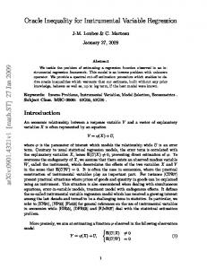
Fig. 1. (a) First sinusoidal source sequence. (b) Second sinusoidal source sequence. (c) Signal Source A + Source B. (d) First-order AR noise ( = 0:6).(e) Raw data sequence = Signal C + noise D. (f) Reconstructed signal using RIVST 2. (g) Corresponding reconstruction error. (h) Reconstructed signal using RIVST 3. (i) Corresponding reconstruction error.

A. Low-Rank IV Parameter Estimation and Adaptive Filtering The modified normal equations of IV parameter estimation are defined as (see, e.g., [20, p. 120]): (30) is the estimated RIV cross covariance vector where with time update (31)

and is the actual sample of a reference signal. is the desired RIV parameter vector of dimension . In the classical system identification literature, the usual represents an invertible matrix. In assumption is that this case, the solution is formally expressed as (32) It is ultimately clear that the invertibility assumption of must limit the practical value of the method. Robust imple-

2716

IEEE TRANSACTIONS ON SIGNAL PROCESSING, VOL. 46, NO. 10, OCTOBER 1998

(a)

(b) Fig. 2. Singular value trajectories for the experiment shown in Fig. 1. (a) Estimated singular value trajectories for the algorithm RIVST 2. (b) Estimated singular value trajectories for the algorithm RIVST 3. Dashed horizontal linesindicate fixed singular value threshold.

mentations of the RIV method require that the dimensions of are determined larger or much larger than the actual number of dominant modes in the signal (overmodeling). Thus, in the following, we consider the overmodeling case, where . The inverse matrix in (32) is formallly replaced by the rank Moore–Penrose pseudoinverse (5b) as

will approximate the Moore–Penrose pseudoinverse sufficiently closely. It can be shown that a Schur pseudoinverse also satisfies the Moore–Penrose conditions [9]. Using the Schur pseudoinverse, an estimate of the low-rank RIV parameter vector at time can be defined as

(33) is easily constructed using the An approximation to elements of a RIV subspace tracker. It can be expected that the following Schur pseudoinverse [9] (34)

(35) The practical computation of

can be accomplished via

back substitution

(36a) (36b)

STROBACH: BI-ITERATION RECURSIVE INSTRUMENTAL VARIABLE SUBSPACE TRACKING AND ADAPTIVE FILTERING

2717

(a)

(b) Fig. 3. Rank trajectories corresponding to the singular value trajectories of Fig. 2. (a) Estimated rank trajectory for RIVST 2. (b) Estimated rank trajectory for RIVST 3.

(36c) can be The estimated low-rank RIV parameter vector used to compute the low-rank RIV subspace adaptive filter as (37) Note, however, that it is not necessary to compute the esexplicitly if timated low-rank RIV parameter vector only adaptive filtering is an issue. Alternatively to (37), we may compute (38a)

vector is avoided. Note that this solution makes a heavy use of “data compression” principles as it is assumed implicitly that both and can be mapped into a subspace of with little or no information loss. dimension A final issue is the efficient computation of the cross covariance compressor (36a). We show that the compressed can also be updated RIV cross covariance vector efficiently in time. To see this, premultiply both sides of the RIV cross covariance vector time update equation (31) by as

(38b) and the explicit quantification of the low-rank RIV parameter

(39)

2718

IEEE TRANSACTIONS ON SIGNAL PROCESSING, VOL. 46, NO. 10, OCTOBER 1998

=

Fig. 4. (a) First sinusoidal source sequence. (b) Second sinusoidal source sequence. (c) Signal Source A + Source B. (d) First-order AR noise ( = 0:9). (e) Raw data sequence = Signal C + noise D. (f) Reconstructed signal using RIVST 2. (g) Corresponding reconstruction error. (h) Reconstructed signal using RIVST 3. (i) Corresponding reconstruction error.

Further, use (23a) to establish the following time updating recursion for the transposed compressor matrix:

Finally, exploit the fact that ing to (25). This yields

accord-

(40) Now, substitute (40) into (39) to obtain (42) B. Low-Rank RIV Adaptive Filtering Without Reference Signal (41)

In some applications, such as time series adaptive filtering, the reference signal is simply a shifted version of the data.

STROBACH: BI-ITERATION RECURSIVE INSTRUMENTAL VARIABLE SUBSPACE TRACKING AND ADAPTIVE FILTERING

2719

(a)

(b) Fig. 5. Singular value trajectories for the experiment shown in Fig. 4. (a) Estimated singular value trajectories for the algorithm RIVST 2. (b) Estimated singular value trajectories for the algorithm RIVST 3. Dashed horizontal linesindicate fixed singular value threshold.

In this case, low-rank adaptive filtering reduces to a simple onto the column orthogonal projection of the data vector . Since the columns of represent space of the fundamental modes of the signal, we can expect that this of the orthogonal projection will produce an estimate desired signal in the data as

estimates of subsequent time steps in a “layered” fashion according to

.. .

(44a) (44b)

(43) of dimension This way, we obtain a signal vector estimate in each time step of the recursion. In time series adaptive filtering, it is convenient to combine these signal vector

is extracted from The actual estimated signal sample via bottom pinning the “layered” signal vector estimate according to (44b). See [9], [11], [18], and the next section for details on layered subspace adaptive filtering.

2720

IEEE TRANSACTIONS ON SIGNAL PROCESSING, VOL. 46, NO. 10, OCTOBER 1998

(a)

(b) Fig. 6. Rank trajectories corresponding to the singular value trajectories of Fig. 5. (a) Estimated rank trajectory for RIVST 2. (b) Estimated rank trajectory for RIVST 3.

C. Rank Adaptivity and Aspects of Practical Implementation A simple fixed rank implementation of the discussed RIV subspace trackers and adaptive filters is usually not the optimal solution in practice because the number of independent sources or dominant fundamental modes in the data may vary with time. A maximum number of dominant fundamental modes that can be expected in a specific application is usually always known from practical side conditions. This suggests that the rank adaptivity problem is solved in the following way. 1) The RIV subspace trackers are always operated with a sufficiently large fixed-rank dimension . 2) The signal-excited dimensions in the preselected subspace of dimension are then identified by comparing

the diagonal elements of the triangular matrix with a fixed threshold. Recall that the diagonal elements are the estimated singular values of the RIV of cross-covariance matrix according to (8). Further, recall that the associated singular values of signal-free subspace dimensions should vanish completely in the ideal case because shifted noise vectors are correlated out in the RIV cross covariance matrix. In practice, we still obtain some nonzero subdominant singular values due to deviations from ideal conditions and finite observation intervals. Experiments have revealed, however, that these subdominant singular values are usually small in magnitude and almost independent from temporal

STROBACH: BI-ITERATION RECURSIVE INSTRUMENTAL VARIABLE SUBSPACE TRACKING AND ADAPTIVE FILTERING

2721

Fig. 7. (a) Sequence of chirp transients. (b) First-order AR noise ( = 0:6). (c) Raw data = chirp sequence A + noise B. (d) Reconstructed chirp sequence using RIVST 3. (e) Reconstruction error.

Fig. 8. Estimated singular value trajectories for the experiment shown in Fig. 7. Dashed line indicates fixed singular value threshold.

variations of the data power. Therefore, it is usually sufficient to suppress these subdominant singular values with a fixed threshold. The following algorithm compares the diagonal elements of with a fixed threshold . A rank estimate is of dimension is computed, and a pinning matrix constructed as

Verify that a generated in this fashion can be used to concentrate the singular vectors of the signal-excited dimencolumns of a compacted subspace basis sions in the first as matrix (46) Hence, in a rank adaptive implementation of the layered RIV subspace adaptive filter, we use only the signal-excited dimensions of the subspace as

for if

then (47)

(45) endif

where

comprises the first

elements of

.

2722

IEEE TRANSACTIONS ON SIGNAL PROCESSING, VOL. 46, NO. 10, OCTOBER 1998

Fig. 9.

Estimated rank trajectory for the experiment shown in Fig. 7.

Fig. 10. (a) Sequence of chirp transients. (b) First-order AR noise ( = 0:9). (c) Raw data = chirp sequence A + noise B. (d) Reconstructed chirp sequence using RIVST 3. (e) Reconstruction error.

In the same fashion, the method can be applied for rank adaptive RIV parameter estimation as well.

V. EXPERIMENTAL VERIFICATION The RIV subspace tracking algorithms proposed in this paper have been tested experimentally. We show results from an application in time series adaptive filtering using the layered RIV subspace adaptive filter described in the previous section. The goal in our experiments is the sequential reconstruction of two superimposed transient sinusoids in additive stationary Gaussian noise with unknown correlation. The reconstruction capability for nonstationary chirp signals in stationary Gauss-

ian noise with unknown correlation is also demonstrated. All experiments shown in this section have been carried out for the case of a square RIV cross covariance matrix, i.e., we throughout all experiments. In all cases, the assume is generated as vector that instrumental variable vector is shifted by time steps relative to the data vector . Fig. 1 shows the data components used in a first series of experiments. Fig. 1(a) is a first transient sinusoidal sequence with normalized frequency . This source is active in the time interval . Fig. 1(b) shows the signal . This of a second source with normalized frequency . Fig. 1(c) source is active in the time interval is the sum of the two source signals. Fig. 1(d) is a first-order

STROBACH: BI-ITERATION RECURSIVE INSTRUMENTAL VARIABLE SUBSPACE TRACKING AND ADAPTIVE FILTERING

Fig. 11.

2723

Estimated singular value trajectories for the experiment shown in Fig. 10. Dashed line indicates fixed singular value threshold.

Fig. 12.

Estimated rank trajectory for the experiment shown in Fig. 10.

AR noise process with correlation . Fig. 1(e) is the sum of the signal in Fig. 1(c) and the noise in Fig. 1(d). The signal-to-noise ratio (SNR) is 0 dB for each source. The algorithms RIVST 2 (Table II) and RIVST 3 (Table III) are used for subspace tracking. Signal reconstruction is accomplished using the rank adaptive layered RIV subspace adaptive filtering concept as described in the previous section. Fig. 1(f) is the reconstructed signal using the algorithm RIVST and . We used an 2 with “advanced” version of the data with a shift of as an instrumental variable sequence. In other words, the data sequence is delayed by 300 time steps relative to the instrumental variable sequence. Fig. 1(g) is the corresponding reconstruction error sequence [difference between curves in

Fig. 1(c) and Fig. 1(f)]. This experiment is repeated using the ultra-fast algorithm RIVST 3 in the same parameter configuration. Fig. 1(h) is the reconstructed signal, and Fig. 1(i) is the corresponding reconstruction error. It can be seen that RIVST 3 produces virtually the same or almost the same reconstruction result as the more complex algorithm RIVST 2. Details about the internal operation of the algorithms are displayed in Fig. 2, where the trajectories of the four estimated dominant singular values (main diagonal elements of ) are shown for the two experiments. Fig. 2(a) shows the estimated singular value trajectories of RIVST 2, and Fig. 2(b) shows the estimated singular value trajectories of RIVST 3. The dashed horizontal lines indicate the fixed threshold that is used for singular value discrimination. It

2724

IEEE TRANSACTIONS ON SIGNAL PROCESSING, VOL. 46, NO. 10, OCTOBER 1998

becomes apparent that the spurious singular values in the silent areas are relatively small in magnitude, as expected. Thus, it is not difficult to discriminate the signal from the noise in this example. Fig. 3 shows the corresponding estimated rank trajectories. The problem becomes more difficult with increasing noise correlation. In a second experiment, the performance of the algorithms is studied using a data set where the superimposed . All other first-order AR noise has a correlation of parameter configurations of the algorithms remain unchanged. Fig. 4 shows the raw data components, the reconstruction results, and the reconstruction errors. Again, we find that the algorithms RIVST 2 and RIVST 3 perform almost identically. Fig. 5 shows the corresponding estimated singular value trajectories. It can be seen that highly correlated noise processes produce larger spurious singular values in the silent areas where the sources are inactive. In general, a reliable operation in highly correlated noise requires that the filter order is chosen sufficiently large. In addition, the observation intervals should be long. This means that practical values for the exponential forgetting factor should be relatively close must be large to ensure a sufficient to 1, and the delay “decoupling” of the shifted noise processes. Fig. 6 finally shows the estimated rank trajectories for this experiment. In a last experiment, we use the layered RIV subspace adaptive filter for reconstruction of a nonstationary transient chirp signal from noisy observations. In this experiment, the main assumption that shifted versions of the signal span identical subspaces is clearly violated for the transient chirp signals. It should be investigated how the algorithms perform under such imperfect conditions. Again, we use an advanced version of the data as an instrumental variable sequence. The critical parameter is the shift . In general, the value of should be chosen sufficiently large to decouple the noise. On must be sufficiently small to ensure that the other hand, the shifted versions of the signal still span at least almost the same subspace. For a nonstationary signal, these are clearly two contradictory demands. Experiments have confirmed that for nonstationary signals like the chirp, it is usually more important to ensure that shifted versions of the signal span almost the same subspace. Thus, the shift parameter should be set to relatively small values. Fig. 7 shows the raw data and the reconstruction results of a first experiment using the chirp signals. Fig. 7(a) is the chirp sequence. Fig. 7(b) is a first-order AR noise sequence . Fig. 7(c) is the raw data [sum of with correlation the signal in Fig. 7(a) and noise in Fig. 7(b)]. Fig. 7(d) is the reconstruction result, and Fig. 7(e) is the reconstruction error using the algorithm RIVST 3 with parameter configuration and . Fig. 8 shows the corresponding estimated singular value trajectories for this experiment. The dashed horizontal line indicates the fixed singular value threshold. The noise correlation is relatively low, and therefore, the spurious singular values in the silent areas stay far below the singular value threshold. Detection and reconstruction of the signal is hence not difficult in this example. Fig. 9 shows the corresponding estimated rank trajectory.

The experiment is repeated with increased noise correlation . Again, we used the algorithm RIVST 3 with an unchanged parameter configuration. Fig. 10 shows the signal, noise, and data components, the reconstruction result, and the corresponding reconstruction error. It is seen that now, it becomes much more difficult to discriminate the transients from the highly correlated noise sequence. This is confirmed by the estimated singular value trajectories displayed in Fig. 11. The spurious singular values are larger. They even exceed the singular value threshold at some places. Fig. 12 is the corresponding estimated rank trajectory. Clearly, a noise sequence would require a much larger value for the shift parameter . On the contrary, the value of must be small to ensure sufficiently close subspaces of the shifted nonstationary signal. These practical constraints mark the limitations of the RIV subspace method in the processing of noisy transient signals.

VI. CONCLUSION In this paper, we introduced a new class of RIV subspace trackers based on the Bi-SVD concept. These algorithms are highly structured and require only standard matrix operations factorization and matrix-vector multiplication, which like are all operations whose numerical properties are now well understood. Moreover, we developed a class of RIV subspace adaptive filters. These algorithms can be used for sequential reconstruction of signals buried in Gaussian noise with unknown correlation. Detailed computer experiments substantiated the theoretical results. REFERENCES [1] R. O. Schmidt, “Multiple emitter location and signal parameter estimation,” in Proc. RADC Spectrum Estimation Workshop, 1979, pp. 243–258. [2] R. Kumaresan and D. W. Tufts, “Estimating the angles of arrival of multiple plane waves,” IEEE Trans. Aerospace Electron. Syst., vol. AES-19, pp. 134–139, 1983. [3] R. Roy and T. Kailath, “ESPRIT—A subspace rotation approach to estimation of parameters of cisoids in noise,” IEEE Trans. Acoust., Speech, Signal Processing, vol. ASSP-34, pp. 1340–1342, Oct. 1986. [4] P. Stoica and K. C. Sharman, “Maximum likelihood methods for direction-of-arrival estimation,” IEEE Trans. Acoust., Speech, Signal Processing, vol. 38, pp. 1132–1143, July 1990. [5] P. Strobach, “Fast recursive orthogonal iteration subspace tracking algorithms and applications,” Signal Process., vol. 59, no. 1, pp. 73–100, May 1997. [6] D. W. Tufts and R. Kumaresan, “Frequency estimation of multiple sinusoids: Making linear prediction perform like maximum likelihood,” Proc. IEEE, vol. 70, pp. 975–989, Sept. 1982. [7] P. Strobach, “Fast recursive low-rank linear prediction frequency estimation algorithms,” IEEE Trans. Signal Processing, vol. 44, pp. 834–847, Apr. 1996. [8] , “Fast recursive eigensubspace adaptive filters,” in Proc. ICASSP, Detroit, MI, May 1995, pp. 1416–1419. [9] , “Low rank adaptive filters,” IEEE Trans. Signal Processing, vol. 44, pp. 2932–2947, Dec. 1996. [10] P. Comon and G. H. Golub, “Tracking a few extreme singular values and vectors in signal processing,” Proc. IEEE, vol. 78, pp. 1327–1343, Aug. 1990. [11] P. Strobach, “Bi-iteration SVD subspace tracking algorithms,” IEEE Trans. Signal Processing, vol. 45, pp. 1222–1240, May 1997. [12] T. S¨oderstr¨om and P. Stoica, Instrumental Variable Methods for System Identification. Berlin, Germany: Springer-Verlag, 1983. [13] , System Identification. London, U.K.: Prentice-Hall, 1989.

STROBACH: BI-ITERATION RECURSIVE INSTRUMENTAL VARIABLE SUBSPACE TRACKING AND ADAPTIVE FILTERING

[14] B. Friedlander, “Instrumental variable methods for ARMA spectral estimation,” IEEE Trans. Acoust., Speech, Signal Processing, vol. ASSP31, pp. 404–414, Apr. 1983. [15] M. Viberg, P. Stoica, and B. Ottersten, “Array processing in correlated noise fields based on instrumental variables and subspace fitting,” IEEE Trans. Signal Processing, vol. 43, pp. 1187–1199, May 1995. [16] F. L. Bauer, “Das Verfahren der Treppeniteration und verwandte Verfahren zur L¨osung algebraischer Eigenwertprobleme,” Z. Angew. Math. Phys., vol. 8, pp. 214–235, 1957. [17] P. Strobach, Linear Prediction Theory: A Mathematical Basis for Adaptive Systems, Springer Series in Information Sciences. New York: Springer-Verlag, 1990, vol. 21. , “Square hankel SVD subspace tracking algorithms,” Signal [18] Process., vol. 57, no. 1, pp. 1–18, Feb. 1997. [19] P. Stoica, M. Viberg, M. Wong, and Q. Wu, “A unified instrumental variable approach to direction finding in colored noise fields,” Tech. Rep. CTH-TE-32, Chalmers Univ. Technol., Gothenburg, Sweden, July 1995; in Digital Signal Processing Handbook. Boca Raton FL: CRC, 1996. [20] T. C. Hsia, System Identification. Lexington, MA: Lexington Books, 1977. [21] T. Gustafsson and M. Viberg, “Instrumental variable subspace tracking with applications to sensor array processing and frequency estimation,” in Proc. 8th IEEE Signal Processing Workshop SSAP, Corfu, Greece, June 1996, pp. 78–81. [22] T. Gustafsson, “On subspace-based instrumental variable methods with applications to time-varying systems,” Tech. Rep. 234L, Dept. Applied Electron., Chalmers Univ. Technol., G¨oteborg, Sweden, 1996.

2725

[23] G. H. Golub and C. F. Van Loan, Matrix Computations, 2nd ed. Baltimore, MD: John Hopkins Univ. Press, 1989. [24] G. W. Stewart, “Methods of simultaneous iteration for calculating eigenvectors of matrices,” in Topics in Numerical Analysis II, J. H. Miller, Ed. New York: Academic, 1975, pp. 169–185. [25] B. N. Parlett and W. G. Poole, “A geometric theory for the QR; LU and power iterations,” SIAM J. Numer. Anal., vol. 10, no. 2, pp. 389–412, Apr. 1973.

Peter Strobach (M’86–SM’91) received the Engineer’s degree in electrical engineering from Fachhochschule Regensburg, Regensburg, Germany, in 1978, the Dipl.-Ing. degree from Technical University Munich, Munich, Germany, in 1983, and the Dr.-Ing. (Ph.D.) degree from Bundeswehr University, Munich, in 1985. From 1976 to 1977, he was with CERN Nuclear Research, Geneva, Switzerland. From 1978 to 1982, he was with Messerschmidt–Boelkow–Blohm GmbH, Munich. From May 1986 to December 1992, he was with Siemens AG, Zentralabteilung Forschung und Entwicklung (ZFE), Munich. Currently, he is with Fachhochschule Furtwangen, R¨ohrnbach, Black Forest, Germany. Dr. Strobach is a member of the IEEE Signal Processing Society and an Editorial Board member of Signal Processing. He is a Member of the New York Academy of Sciences and is listed in Who’s Who in the World.