Paulo R.S. Mendonça, Dirk Padfield, James Miller, and Matt Turek. GE Global Research. One Research Circle. Niskayuna, NY 12309. {mendonca,padfield ...
Bias in the Localization of Curved Edges Paulo R.S. Mendon¸ca, Dirk Padfield, James Miller, and Matt Turek GE Global Research One Research Circle Niskayuna, NY 12309 {mendonca,padfield,millerjv,turek}@research.ge.com
Abstract. This paper presents a theoretical and experimental analysis of the bias in the localization of edges detected from the zeros of the second derivative of the image in the direction of its gradient, such as the Canny edge detector. Its contributions over previous art are: a quantification of the localization bias as a function of the scale σ of the smoothing filter and the radius of curvature R of the edge, which unifies, without any approximation, previous results that independently studied the case of R � σ or σ � R; the determination of an optimal scale at which edge curvature can be accurately recovered for circular objects; and a technique to compensate for the localization bias which can be easily incorporated into existing algorithms for edge detection. The theoretical results are validated by experiments with synthetic data, and the bias correction algorithm introduced here is reduced to practice on real images.
1
Introduction
Edge detection is a basic problem in early vision [16,21], and it is an essential tool to solve many high-level problems in computer vision, such as object recognition [25,20], stereo vision [17,1], image segmentation [13], and optical metrology [7]. In the application of edge detection to such high-level problems the criteria relevant to edge detector performance, as stated by Canny [5], are: 1) low error rate, meaning that image edges should not be missed and that false edges should not be found, and 2) good edge localization, meaning that the detected edge should be close to the true edge. The former criterion is dealt with in works such as [6,14,10]. It is this latter requirement that this research effort seeks to address. In particular, we quantify the error in edge localization as a function of the edge curvature. This error occurs even for noise-free images, and therefore the effect of noise was not considered in this paper. With the exception of non-linear methods such as anisotropic diffusion [19], edge detection can almost invariably be reduced to convolution with a Gaussian kernel with given scale parameter σ and computation of image gradients. For an ideal one-dimensional step [12] or for a two-dimensional step with rectilinear boundary [15], the location of a noise-free isolated edge can be exactly determined, and bounds can be provided for the error in the edge location in the presence of noise. However, when these models are applied to the analysis of the detection of curved edges in two-dimensions, effects due to the interaction between the kernel and the curved edges are not accurately captured. This problem has been tackled in previous works for particular intervals of σ and the T. Pajdla and J. Matas (Eds.): ECCV 2004, LNCS 3022, pp. 554–565, 2004. c Springer-Verlag Berlin Heidelberg 2004 �
Bias in the Localization of Curved Edges
(a) σ = 0.00R
(b) σ = 0.30R
(c) σ = 0.54R
(d) σ = 0.70R
(e) σ = 0.80R
(f) σ = 1.00R
555
Fig. 1. Canny edges, points of which are shown as white asterisks, detected on the images of a circle with constant radius R = 10 smoothed by Gaussian kernels of different standard deviations σ. The true location of the edge is shown as a solid curve. For σ = 0.00R (a), the points along the detected edge coincide with the solid curve. It can be seen that the detected edge moves towards the center of curvature of the true edge as σ increases (b), until it reaches a critical value σ = σc = 0.54R (c) (see section 3.2). It then begins to move away from the center of curvature (d), and intercepts the true edge when σ = σ0 = 0.80R (e) (see, again, section 3.2). The detected edge continues to move outwards as σ grows (f).
edge curvature [2,22,23], but the theoretical and experimental characterization of these effects for the full range of values of the scale σ is first introduced in this paper. The results presented here show that the extent to which detected edges move from their ideal positions can be determined and reduced based on the scale parameter of the smoothing kernel and the radius of curvature of the detected edge. The prescription of an optimal scale for accurate estimation of edge location is also introduced. Section 2 presents the mathematical results which are used throughout the remainder of the paper. An analysis of the bias in the localization of edges as a function of the scale of the smoothing kernel and the curvature of the edge is shown in section 3, which also brings an experimental validation of the theoretical derivations and analyzes effects that occur at certain critical values for the scale parameter σ. Section 4 introduces a method for correcting the localization bias. Experimental results are given in section 5, followed by a conclusion and proposals for future work in section 6.
2 Theoretical Background The simplest 2D model that can be used to analyze errors in the localization of curved edges is a circle, since its border has constant curvature. The limit case of zero curvature
556
P.R.S. Mendon¸ca et al.
corresponds to the analysis of step edges, which can be carried out either implicitly, as in [5], which considered 1D step edges, or explicitly, as in [10]. The main steps common to most algorithms for edge detection, such as the ones cited in section 1, are image smoothing by convolution with an appropriate kernel, usually Gaussian, the computation of derivatives of the image, and the localization of peaks of the first derivative or, equivalently, zeros of the second derivative. Convolution and differentiation commute, and their combined effect is that of convolving the image with derivatives of the Gaussian kernel. The operation of convolution in space is equivalent to multiplication in the frequency domain, and therefore a brief review of some results regarding the Fourier analysis of circularly symmetric signals will be presented. First, recall that the Fourier transform�of a circularly symmetric function is also 2 2 circularly symmetric, i.e., pair, � F (w1 , w2 ) are a Fourier � if f (x, y) = f ( x + y ) ↔ � 2 2 2 2 2 then F (w1 , w2 ) = F ( w1 + w2 ). Moreover, if r = x + y and ρ = w1 + w22 , then � ∞ rf (r)J0 (ρr)dr and (1) F (ρ) = 2π �0 ∞ 1 f (r) = ρF (ρ)J0 (rρ)dρ, (2) 2π 0 where Jn (·) is the nth-order Bessel function of the first kind. Consider the function s : R2 → R given by � 1 if x2 + y 2 ≤ R2 , (x, y) �→ s(x, y) = 0 otherwise.
(3)
This function is a circularly symmetric pulse, and its representation in polar coordinates, s : R+ × [0, 2π) → R, is given by � 1 if r ≤ R, (r, θ) �→ s(r, θ) = s(r) = (4) 0 otherwise. Using (1), the Fourier transform of s(r), denoted by S(ρ), can be found as S(ρ) =
2πR J1 (Rρ). ρ
(5) x2 +y 2
− 2σ2 1 . The function k(x, y) Now let k(x, y) be a Gaussian kernel, i.e., k(x, y) = 2πσ 2e is circularly symmetric, i.e., k(x, y) = k(r), and therefore its Fourier transform can be computed from (1), resulting in K(ρ) given by
K(ρ) = e
−σ 2 ρ2 2
.
(6)
ˆ The product S(ρ) of (5) and (6) is 2πR −σ2 ρ2 ˆ e 2 J1 (Rρ), S(ρ) = ρ
(7)
Bias in the Localization of Curved Edges
557
and, therefore, using (2), the result sˆ(r) of smoothing the function s(r) with the Gaussian kernel k(r) will be given by � sˆ(r) = R
∞
0
e
−σ 2 ρ2 2
J0 (rρ)J1 (Rρ)dρ.
(8)
Although (8) cannot be computed in closed form, its derivatives can [24]. This observation was central for the development of this work. The first and second derivatives of (8) are shown below: � � dˆ s Rr R −(r2 +R2 ) and (9) = − 2 e 2σ2 I1 dr σ σ2 � � � �� � �� 2) d2 sˆ r Rr R Rr R −(r2 +R 1 2σ 2 I − , (10) = − e + I 1 0 2 2 2 2 2 dr σ σ r σ σ σ2 where In (·) is the modified Bessel function of order n. The problem of edge detection can be stated now as the search for the zeros of (10).
3
Bias in Edge Localization
Fig. 1 shows the experimental results of running a Canny edge detector on the image of a circularly symmetric pulse of radius R = 10 at scales σ = 0.00R, 0.30R, 0.54R, 0.70R, 0.80R, and 1.00R. These results were obtained by generating a synthetic image of a disc. Partial volume effects were taken into account by subsampling pixels near the edge of the circle and counting the number of inside and outside samples. For each value of the scale σ of the Gaussian smoothing filter a Canny edge detector with subpixel accuracy was run on the images. The mean distance from these points to the center of the circle was then computed and declared to be the detected radius. It can be seen that, even in the absence of noise, the detection of edges by computing the zeros of the second derivative of an image in the direction of its gradient produces a shift in the localization of the edges, which is a well-known effect [21]. By repeating this experiment at various realistic levels of resolution and quantization, it was found that these parameters have minimal influence on localization accuracy. The results in [22,23] show that, if R � σ, the shift in the location of edges will be towards their center of curvature. In [8,9], a similar result was found by using a pair of straight edges with a common endpoint and varying intersection angle as the model for the analysis. In the case were R � σ, the analysis in [2] shows that the shift will be in the opposite direction, the so called “expansion phenomenon” discussed in section 3.2. These works did either purely numerical or approximate analytical studies and proposed independent remedies to the problem. The analysis in section 3.2 will unify these results, producing an exact result for the shift in edge location that is valid for any value of R/σ. An important observation is that if r0 is a zero of (10), the value of r0 /σ depends only on the ratio R/σ, i.e., if the radius of the pulse and the scale of the smoothing kernel are multiplied by a common factor, the value of r0 will be multiplied by the same factor.
558
P.R.S. Mendon¸ca et al. 1
0.5
s ds/dr d2s/dr2
0.5
s ds/dr d2s/dr2
0.4 0.3 Amplitude
Amplitude
0.2 0
−0.5
0.1 0 −0.1 −0.2
−1
−0.3 −1.5 0
0.5
1
1.5 r
2
2.5
3
−0.4 0
(a) σ = 0.54R
0.5
1
1.5 r
2
2.5
3
(b) σ = 1.00R
Fig. 2. Profiles of a smothed circular pulse and its derivatives along the radial direction. The amplitude of the pulse is 1 and its radius R is 1. The profiles are shown as a function of r, as in (8). The circle marks the ideal location for the edge of the pulse, and the asterisk indicates the location of an edge corresponding to the zero crossing of the second derivative of the pulse. Comparing the position of the zero-crossings with the ideal locations of the edges, it can be seen that when σ = 0.54R the radius of the edge is underestimated by 9.6%, whereas for σ = 1.00R the radius is overestimated by 14.5%. Observe that the full 2D pulse and its derivatives in the direction of its gradient can be obtained by rotating the respective curves around the vertical axis of the plots. The experimental results shown in Fig. 1 produced, for σ = 0.54R, an underestimation of the radius of curvature of 9.7%, and for σ = 1.00R an overestimation of 14.7%. The small deviation from the theoretical predictions are attributable to sampling and quantization.
3.1
Theoretical versus Experimental Bias
Fig. 2 shows a plot of (8) for a pulse with radius R = 1.0 smoothed by a Gaussian kernel with scale σ = 0.54R in (a) and σ = 1.00R in (b). The images also show the first and second derivatives of the pulse as functions of r, as given by (9) and (10). The zero-crossings are, in both cases, indicated by asterisks, and the true positions of the edges are marked by a circle. The location of the detected edge underestimates the true radius by 9.6% when σ = 0.54R, and overestimates it by 14.5% when σ = 1.00R. These results can be compared with the experimental errors obtained for the detected radius in Fig. 1, which were 9.7% of underestimation when σ = 0.54R and 14.7% of overestimation when σ = 1.00R. The small deviation is due to effects not considered in the theoretical model, such as sampling and quantization. It is clear that there is a variable offset in the location of edges obtained by an edge detector based on zero crossings of the second derivative in the gradient direction. Contrary to what is commonly believed, this offset can produce either under- or overestimation of the edge’s radius of curvature, unifying the results in [2,22,23]. 3.2
Critical Values of σ
As σ varies in the interval [0, ∞), which is equivalent to a decrease in the ratio R/σ from ∞ to 0 for a fixed R, it can be seen from Fig. 1 that, initially, the detected edge moves towards the center of curvature of the original edge. As σ increases to a certain
Bias in the Localization of Curved Edges
559
Table 1. Critical values of σ. As σ varies from 0 to 0.543R, the detected edge shifts towards the center of curvature of the true edge, and its radius of curvature r0 varies from R to 0.901R. When σ reaches the critical value of σc = 0.543R, the detected edge begins to move outwards, until it crosses the position of the original edge at σ0 = 0.804R. As σ keeps increasing, the detected edge still moves outwards, until, as σ → ∞, the radius r0 → σ.
σ = σc , the edge reaches a critical point after which it starts moving back towards the location of the original edge. At a particular σ = σ0 > σc , the location of the detected edge coincides with that of the original edge, and as σ keeps increasing, the detected edge continues to shift outwards. The values of R/σ at which these events occur can be directly computed from (9) and (10), as will be shown next. Optimal Scale for Curvature Resolution. The zeros of (10) give the location of the edges of (8). Observe that the function h(r; R, σ) given by � � � � � � r R Rr Rr 1 I1 h(r; R, σ) = − 2 I0 (11) + σ2 r σ2 σ σ2 is the only term that influences the location of the zeros of (10), since the factor −R/σ 2 is constant and the factor exp(−(r2 + R2 )/(2σ 2 )) is positive for all r. The non-zero value of σ that results in minimal bias in edge localization, denoted σ0 , can be found by making r = R in (11) and solving � � 2� � 2� � R R R 1 R I1 − 2 I0 =0 (12) + σ2 R σ2 σ σ2 for σ. Using the substitution R/σ = α, (12) can be rewritten as α2 I0 (α2 ) − (1 + α2 )I1 (α2 ) = 0,
(13)
with solution α ≈ 1.243, i.e., σ0 ≈ 0.804R. The value σ0 is of great importance. The localization of edges with radius R = 1.243σ0 = σ0 /0.804 for any σ0 , although still affected by noise, sampling and quantization, will not be subject to the effect of any curvature-induced bias, according to the theoretical model. This result complements that of [10], which provides a minimum scale σ ˆ at which image gradients can be reliably detected. In that work, however, edges are modeled as steps with rectilinear boundaries, which lead the authors to conclude that [10, section 9] “localization precision improves monotonically as the maximum second derivative filter scale is increased.” This statement is adjusted by the results of this work, which relates localization precision to the curvature of the detected edge.
560
P.R.S. Mendon¸ca et al.
Maximum Shift to the Center of Curvature. To obtain σc it is necessary to find the ∂r simultaneous solution of (11) and ∂σ = 0, i.e., the scale for which the drift velocity [14] of the edge with respect to scale is zero. This condition can be rewritten [11, section 5.6.2] after the appropriate simplification as � � � � � � Rr Rr R σ4 I1 − I = 0. (14) + 3 0 r r R σ2 σ2 By making the substitution R/σ = α and r/σ = β, the simultaneous set of equations given by (11) and (14) becomes � � β 1 I1 (αβ) − I0 (αβ) = 0, (15) + α αβ � � 1 α + I1 (αβ) − I0 (αβ) = 0, (16) β αβ 2 with solution α ≈ 1.842 and β ≈ 1.660. Therefore, the minimum value of r0 is ≈ 0.901R, obtained when σ = σc ≈ 0.543R. The significance of the value σc and the corresponding radius is that they provide a limit to the maximum bias in the direction of the center of curvature, or a one-sided bound to the bias in the localization of an edge as a function of its radius of curvature. Expansion Phenomenon. The expansion phenomenon described in [2] can also be analyzed with the techniques developed here. Assume that σ → ∞, i.e., α → 0, with α and β as in the previous paragraph. The first order Taylor expansion of I1 (x) and I0 (x) are I1 (x) = x/2 and I0 (x) = 1. Substituting these expressions in (15), one obtains � β α
2
αβ β +1 1 + αβ − 1 = 0, producing the result limα→0 β = 1 ⇒ r0 = σ. 2 −1 = 2 This shows that, as σ increases, closed contours will tend to become circles with radius σ, as described in [2]. Table 1 summarizes the critical values of σ and the corresponding values of r0 .
4
Correction of Bias in Edge Localization
Because the value of r0 /σ depends only on the ratio R/σ, it is possible to summarize the relationship between the inputs R and σ and the output r0 in a single one-dimensional plot of (r0 − R)/σ as a function of r0 /σ, shown in Fig. 3. The parameter r0 /σ was chosen as the abscissa for convenience: the curves in Fig. 3 can then be interpreted as a lookup table to correct the position of a point in an edge as a function of the scale σ of the smoothing kernel and the measured radius of curvature of the detected edge at the location of the given point. The dashed and solid curves in the figure represent the theoretical and experimental lookup tables, respectively. This suggests a simple algorithm to correct for curvature-induced bias in the localization of edges. First, edge detection by locating the zero crossings of the second derivative of the image in the direction of its gradient is performed, at a scale σe . Then, the blur parameter σb of the image, sometimes referred to as the point spread function,
Bias in the Localization of Curved Edges
561
Lookup Table to Correct Bias in Edge Localization 1.5 Theoretical Experimental
0.5
0
(r −R)/σ
1
0
−0.5 0 1 2
4
6
8
10 12 r0/σ
14
16
18
20
Fig. 3. Theoretical (dashed line) and experimental (solid line) look up tables to correct the location of edges produced by an edge detector based on finding the zeros of the second derivative of the image in the gradient direction. The theoretical curve was produced by numerically solving (11) for the detected radius r0 , for different values of the ratio R/σ. The experimental curve was obtained by applying a Canny edge detector to an image such as the one shown in Fig. 1(a). The use of this look up table to correct the bias in the localization of edges is described in Alg. 1. The theoretical and experimental curves overlap almost completely.
is estimated by using a method such as the � one in [18]. The combination of σe and σb produces an effective scale σ given by σ = σe2 + σb2 , which represents an estimate of the total smoothing of the image. The radius of curvature r0 of the detected edges is then estimated for each point along the edges by fitting a circle to the point and a number of its closest neighbors. Besides determining the radius of curvature, this procedure also locates the center of curvature, which corresponds to the center of the fitted circle. For each point along the edges, the ratio r0 /σ is computed, and the bias at that point is estimated from the lookup table in Fig. 3. The point is then shifted along the line that connects it to its center of curvature, according to the output of the lookup table. This procedure, summarized in Alg. 1, is repeated for all points in the detected edges.
5
Experimental Results
In order to validate the technique introduced in this paper it is necessary to demonstrate its usefulness for edges of generic shape. The development of the theoretical model assumes circularly symmetric images, and, to put the algorithm to test, an experiment was run on an image with a sinusoidal edge, shown in Fig. 4. The radius of curvature of the ideal sinusoid that separates the light and dark regions spans the interval [2.5, ∞) in pixel units, with the minimum radius being reached at peaks of the edge, and the maximum radius obtained at inflection points. A Canny edge detector was run on the image, and each point along the detected edge was shifted appropriately, according to
562
P.R.S. Mendon¸ca et al.
Algorithm 1 Correction of bias in edge localization. 1: 2: 3: 4: 5: 6: 7: 8: 9:
detect edges as zero-crossings of second derivative in gradient direction with scale σe ; � estimate the image blurring factor σb and the effective scale σ = σe2 + σb2 ; for each point x in detected edges do compute radius of curvature r0 of detected edge at x; compute center of curvature x0 of detected edge at x; compute r0 /σ; determine bias � = (r0 − R)/σ from the lookup table in Fig. 3; correct x by moving it −�σ pixel units in the direction (x − x0 )/�x − x0 �; end for
Alg. 1. The detected edge for σ = 3 is shown as a series of white dots in Fig. 4, and the corresponding corrected points are shown in black. It can be seen that, although still non-zero, the bias has been significantly reduced. To quantify this improvement, the RMS distance between the detected points and the ideal edge was computed before and after correction. For σ = 1, 2, 3 and 4, the original RMS distances were 0.1266, 0.2828, 0.5067 and 0.8097, respectively. After correction, the RMS distances were reduced to 0.1024, 0.1087, 0.2517 and 0.7163. The error is not zero because, even though the curve can be locally approximated by circular patches, the edge is not circularly symmetric as assumed in the model. It is worth noting that, for the commonly used σ values of 1 and 2, the anecdotal standard of 1/10 of a pixel unit in accuracy is achieved only after the application of the technique for bias correction introduced in this paper. An experiment in invariant theory was conducted to evaluate the performance of the algorithm discussed here when applied to real data. Two images of a wrench were acquired at different viewpoints. A Canny edge detector was used to detect edges on the images, each image with a different kernel scale σ = 1.00 and σ = 5.00. The smoothed images and the overlaid edges are shown in Fig. 5. Using the technique developed in
(a)
(b)
Fig. 4. Detection of sinusoidal edges for σ = 3. The radius of curvature of the ideal edge separating the light from dark areas, shown as a solid white line, varies from 2.5 to ∞ in pixel units. The detected and corrected edges are indicated by white and black dots, respectively. Notice the effect of the correction in the zoomed image in (b).
Bias in the Localization of Curved Edges
(a) σ = 1.00
563
(b) σ = 5.00
Fig. 5. Two viewpoints of a wrench used to demonstrate the improvement in accuracy in the detection of edges. Images (a) and (b) were smoothed with scales of 1 and 5, respectively. The detected edge is shown as a thick white line on the border of the wrench. The corrected edges were not shown because, at this resolution, the difference between the detected and corrected edges is not visible.
(a)
(b)
(c)
(d)
Fig. 6. Comparison between the projectively invariant signature of the image contour in Fig. 5(a) (solid line) versus that of Fig. 5(b) (dashed line). Image (a) shows the signatures of the detected edges and image (b) shows the signatures of the corrected edges. Notice that the signatures in image (b) are closer together, indicating that the corrected points are closer to the ideal edge of the wrench. Images (c) and (d) show zoomed in portions of the detected and corrected signatures, respectively. Notice the improvement in image (d) over image (c).
[25], the projectively invariant signatures of the edges of the wrench in each view were computed, as can be seen in Fig. 6(a). Due to the different scales used in the detection of the edges, their invariant signatures are significantly different. This difference is visibly reduced if the edges, before the computation of their respective signatures, are corrected with the algorithm introduced in this paper, as can be seen in Fig. 6(b). Figs. 6(c) and 6(d) show a closer view of the signatures where the improvement is more apparent.
6
Conclusions and Future Work
This paper brings an analysis of the error in the localization of edges detected by computing the zeros of the second derivative of an image in the direction of its gradient. A
564
P.R.S. Mendon¸ca et al.
closed-form expression for the derivative and second derivative of circularly symmetric pulses was presented along with experimental validation. These expressions were used to quantify the bias in the localization of the points of an edge as a function of the edge curvature, and these results were confirmed by experiments with synthetic data. Given the scale and edge curvature, this bias can then be corrected using the lookup table computed as described in this paper. This method of correction was validated using both synthetic and real images. The techniques developed in this paper can be employed in the analysis of other problems in edge detection. A natural candidate would be the analysis of the bias in the localization of edges computed from the zero-crossings of the Laplacian. The Laplacian of any circularly symmetric pulse sˆ(r), as in (8), is given by ∇2 sˆ(r) =
s ∂ 2 sˆ 1 ∂ˆ + . 2 ∂r r ∂r
Substituting (9) and (10) in (17), one easily obtains � � � �� � �� r Rr R Rr R −(r2 +R2 ) 2 I − , + I ∇2 sˆ(r) = − 2 e 2σ2 1 0 σ σ2 r σ2 σ2 σ2
(17)
(18)
an expression which could be used to derive an analysis similar to the one carried out in this paper for the case of the Laplacian detector. Observe that this would be a significant improvement over the methodology used in [4], which provides a closed form solution for the Laplacian response of a disk image only for the central pixel of the pulse, and in [3,8], which model curved edges as two line segments meeting at an angle. Another natural extension of this work is to evaluate the effect of neighboring structures on the localization of edges. Since convolution and derivatives are linear operations, an image composed of any linear combination of concentric pulses si (r), each with its own radius Ri , would have first and second derivatives given by a sum of terms of the form of (9) and (10), respectively, and the techniques developed in this work could again be applied. The effect of noise on the shift in localization should also be studied. The work presented here is primarily theoretical, and further experimentation on real images is needed. The application of this research to the correction of the underestimated area of tubular structures such as airways found by edge detection in CT images is ongoing.
References 1. H. H. Baker and T. O. Binford. Depth from edge and intensity based stereo. In Proc. of the 7th Int. Joint Conf. on Artificial Intell., pages 631–636, Vancouver, Canada, August 1981. 2. F. Bergholm. Edge focusing. IEEE Trans. Pattern Analysis and Machine Intell., 9(6):726–741, November 1987. 3. V. Berzins. Accuracy of laplacian edge detectors. Computer Vision, Graphics and Image Processing, 27(2):195–210, August 1984. 4. D. Blostein and N. Ahuja. A multiscale region detector. Computer Vision, Graphics and Image Processing, 45(1):22–41, January 1989. 5. J. F. Canny. A computational approach to edge detection. IEEE Trans. Pattern Analysis and Machine Intell., 8(6):679–698, November 1986.
Bias in the Localization of Curved Edges
565
6. J. J. Clark. Authenticating edges produced by zero-crossing algorithms. IEEE Trans. Pattern Analysis and Machine Intell., 11(1):43–57, January 1989. 7. D. Cosandier and M. A. Chapman. High-precision target location for industrial metrology. In S. F. El-Hakim, editor, Volumetrics II, number 2067 in Proc. of SPIE, The Int. Soc. for Optical Engineering, pages 111–122, Boston, USA, September 1993. 8. R. Deriche and G. Giraudon. Accurate corner detection: An analytical study. In Proc. 3rd Int. Conf. on Computer Vision, pages 66–70, Osaka, Japan, December 1990. 9. R. Deriche and G. Giraudon. A computational approach for corner and vertex detection. Int. Journal of Computer Vision, 10(2):101–124, April 1993. 10. J. H. Elder and S. W. Zucker. Local scale control for edge detection and blur estimation. IEEE Trans. Pattern Analysis and Machine Intell., 20(7):699–716, July 1998. 11. O. D. Faugeras. Three-Dimensional Computer Vision: A Geometric Viewpoint. Artificial Intelligence Series. MIT Press, Cambridge, USA, 1993. 12. R. Kakarala and A. Hero. On achievable accuracy in edge localization. IEEE Trans. Pattern Analysis and Machine Intell., 14(7):777–781, July 1992. 13. M. Kass, A. Witkin, and D. Terzopoulos. Snakes: Active contour models. Int. Journal of Computer Vision, 1(4):312–331, January 1988. 14. T. Lindeberg. Scale-Space Theory in Computer Vision, volume 256 of The Kluwer International Series in Engineering and Computer Science. Kluwer Academic Publishers, Boston, USA, 1994. 15. E. Lyvers and O. Mitchell. Precision edge contrast and orientation estimation. IEEE Trans. Pattern Analysis and Machine Intell., 10(6):927–937, November 1988. 16. D. Marr and E. Hildreth. Theory of edge detection. Proc. Roy. Soc. London. B., 207:187–217, 1980. 17. D. Marr and T. Poggio. A computational theory of human stereo vision. Proc. Roy. Soc. London B, 204:301–328, 1979. 18. A. P. Pentland. A new sense for depth of field. IEEE Trans. Pattern Analysis and Machine Intell., 9(4):523–531, July 1987. 19. P. Perona and J. Malik. Scale-space and edge detection using anisotropic diffusion. IEEE Trans. Pattern Analysis and Machine Intell., 12(7):629–639, July 1990. 20. C. A. Rothwell, A. Zisserman, D. Forsyth, and J. L. Mundy. Fast recognition using algebraic invariants. In J. L. Mundy and A. Zisserman, editors, Geometric Invariance in Computer Vision, Artificial Intelligence Series, chapter 20, pages 398–407. MIT Press, Cambridge, USA, 1992. 21. V. Torre and T. Poggio. On edge detection. IEEE Trans. Pattern Analysis and Machine Intell., 8(2):147–162, March 1986. 22. L. J. van Vliet and P. W. Verbeek. Edge localization by MoG filters: Multiple-of-Gaussians. Pattern Recognition Letters, 15:485–496, May 1994. 23. P. W. Verbeek and L. J. van Vliet. On the location error of curved edges in low-pass filtered 2-D and 3-D images. IEEE Trans. Pattern Analysis and Machine Intell., 16(7):726–733, July 1994. 24. G. N. Watson. A Treatise on the Theory of Bessel Functions. Cambridge University Press, Cambridge, UK, 1980 reprint of 2nd edition, 1922. 25. A. Zisserman, D. Forsyth, J. L. Mundy, and C. A. Rothwell. Recognizing general curved objects efficiently. In J. L. Mundy and A. Zisserman, editors, Geometric Invariance in Computer Vision, Artificial Intelligence Series, chapter 11, pages 228–251. MIT Press, Cambridge, USA, 1992.