G. Gallo and A. Olkiicii/Bilinear programming: an exact algorithm sufficient condition for optimality is derived. Then an algorithm for finding an optimal solution is ...
Mathematical Programming 12 (1977) 173-194. North-Holland Publishing Company
BILINEAR P R O G R A M M I N G :
AN E X A C T A L G O R I T H M *
Giorgio G A L L O Istituto per le Applicazioni del Calcolo, Rome, Italy
Aydin O L K O C O * * University of California, Berkeley, U.S.A. Received 9 November 1973 Revised manuscript received 27 January 1976 The Bilinear Programming Problem is a structured quadratic programming problem whose objective function is, in general, neither convex nor concave. Making use of the formal linearity of a dual formulation of the problem, we give a necessary and sufficient condition for optimality, and an algorithm to find an optimal solution.
0. Introduction
The Bilinear P r o g r a m m i n g Problem, in its general form, is to determine x, an n-vector, and y, an n'-vector, to maximize
cTx + x-r QXy + dry,
subject to
A x 0,
Bry 0,
where A is an m by n matrix, B T an rn' by n' matrix, QT an n by n' matrix, c, d, a and b are n, n', m m ' - v e c t o r s respectively. We will assume that X = {x [ A x 0} and Y = {y I BTy 10} are bounded and nonempty. It can be easily verified that the set of all optimal solutions of (0.1) contains at least one element (x*, y*), such that x* is a vertex of X and y* is a vertex of Y. It can be directly derived f r o m the Duality T h e o r y that (0.1) is equivalent to the problem of determining x, an n-vector, and u, an m ' - v e c t o r , to maximize
(crx + min b TU),
subject to
Ax0,
Bu>id+Qx,
(0.2)
u~>0.
In this paper, we solve (0.2) directly. First, in Sections 1 and 2, some geometric properties of the solution set are determined, and a necessary and * Research partially supported by the Office of Naval Research under Contract N00014-69-A-02001010 with the University of California. ** Currently with Consultants Computation Bureau, San Francisco, California. 173
174
G. Gallo and A. Olkiicii/Bilinearprogramming: an exact algorithm
sufficient condition for optimality is derived. Then an algorithm for finding an optimal solution is presented in Section 3, and a discussion on the convergence is given in Section 4. Section 5 consists of a cutting-plane version of the algorithm. A numerical example, a comparison with existing algorithms and computational results are included in Appendices A, B and C respectively.
1. Preliminaries
The basic definitions in this paper are the ones which are most commonly used in the literature (e.g. [4]). Let us define P = {(x, u ) l A x 1 d + Qx; (x, u) ~> 0}, A = {(x, u) I (x, u) ~ P ; bru 1 d + Qx; u >1O} is nonempty f o r any x E R".
Proof. Since Y is nonempty and bounded, max {(d + Qx)ry I Y ~ Y} is bounded. The result follows from the Duality Theory. Lemma 1.1.2. A consists of the union of a set of faces of P.
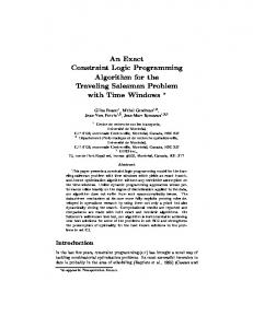
/d×+ du
Fig. 1. The set of optimal solutions of a bilinear programming problem is not necessarily connected.
G. Gallo and A. Ulkiicii/Bilinearprogramming: an exact algorithm
175
Proof. First, we want to show that if a face, F, of P contains, in its relative interior, a point which is in A, then F is included in A. The assertion obviously holds if F is a 0-dimensional face. Let us now assume that F is a d-dimensional face, with d ~> 1, and (x °, u °) is a point in the interior of F belonging to A. Let (x 1, u ~) be an arbitrary point of F ; there exists a point, (x 2, u2), in F such that
( x ° , u ° ) = X ( x l , u~)+(1-;~)(x2, u2);
0~d+Qx,
-bru>~-~.+crx,
u>~O.
(2.1)
Proof. (--~): This part of the proof directly follows from L e m m a 1.1.1 and from the optimality of (2, ti). (~-): Let (2.1) be feasible for all x in X, and (2, ~) be an optimal solution of (1.1), with (2, u*) a feasible solution of (2.1). Since (2, t~) E A, br~ ~ bru *. From optimality of (2, ~) it follows cr2 + brfi i> crg + brti = Z, and by feasibility of (2, u*) ~>~ cr2 +bru*; hence, br~ >~bru *. Then brfi = bru *, and
cr2 + b rl~ --_ cT2 + b Tu * = cr~ + b Ta from which the optimality of (~, ti) follows. Let V = {x 1, x 2. . . . . x k} be a finite set of points in X. Define: d
where z ( V ) = max {crxi + b rui ] x i E V, (x i, u i) ~ A}. Let us define S ( V ) = { x l 3 u > > - O : B u > ~ d ( g ) + Q x } . Theorem 2.1 as follows.
We
can now restate
Theorem 2.1.a. Given V = {x 1. . . . . x k} C_X and U = {(x 1, u 1). . . . . (x k, uk)} C_A, U contains an optimal solution of (1.1) if and only if for each x E X there exists a u
such that Bu>~d(V)+Ox,
u>~O
(2.2)
i.e., S ( V ) D_X. The optimality criterion used in the algorithm of this paper is to check whether X is included in S(V). This is a necessary and sufficient condition of optimality by the above theorem. An obvious property of S ( V ) is the monotonicity (i.e., S(V')D_ S ( V ) whenever V ' _ V) that makes S ( V ) tractable from the algorithmic point of view. There is, however, another set which has similar properties. That is
R ( V ) = {x ]3Ai>~O: d ( V ) + Qx 0, i E I, such that ~;i~rA*wi>0, then R ( V ) D X . Since the existence of such A* can easily be checked by P h a s e I of a linear program, utilizing R ( V ) m a y present a short cut in the algorithm for some problems.
3. The algorithm
In this section an algorithm for solving (0.2) is given, which is based on the optimality condition of T h e o r e m 2.1.a. At each iteration of the algorithm a new vertex of X is found for which a corresponding point in A and the value of the objective function are computed. Then a polyhedral set T is built in such a way that, given the set V of the vertices of X already explored, its intersection with X is contained in S ( V ) . The algorithm terminates when the condition X C_ T, which corresponds to the one stated in T h e o r e m 2.1.a, holds. In Section 5 a different version of this algorithm is given. It is based on the same mathematical tools and makes use of a cutting-plane approach. 3.1. The algorithm Step O. P i c k in X a non-degenerate vertex x °, that is, a vertex with exactly n neighboring vertices x l . . . . . x n. (This assumption on x ° is introduced for the sake of simplicity and will be dropped in the next subsection.) For any vertex x i of X, let us call v i the unit vector defining the halfline emanating from x ° and containing x i. L e t V = { x ° , x ~. . . . . x~}, o~ = { v l . . . . . v ~} and A ={to}. Go to step 1. Step 1. If A = ~, the algorithm terminates, and z(V) is the optimum value of the objective function. Otherwise, select a set to = {v ~', . . . . v i"} in A and go to step 2.
178
G. Gallo and A. Olkiicii/Bilinear programming: an exact algorithm
Step 2. Solving a linear p r o g r a m for each j = 1. . . . .
n, c o m p u t e
{)~)= m a x {0ij I x ° + Oiy ij E S(V)}, and go to step 3. Step 3. Find ( A*~ . . . . , A*~,), an optimal e x t r e m e solution of the linear p r o g r a m n
maximize
~ (llOii)ai,, j=l
subject to
x°+ ~
n
Aiivii E X,
j-1
and go to step 4. Step 4. (a) If g~=~ ( 1 / ~ ) a ~ ~< 1, delete the set o) f r o m A, and go to step 1. Include x q in V and u p d a t e z ( V ) . F o r all J (b) O t h e r w i s e , let x q = xi~+ Y~7=~A*v'). J with A~ > 0, g e n e r a t e a set substituting v ° in o) for v'J; then replace o) in A by these new sets. G o to step 1. R e m a r k 1. In order to c o m p u t e z ( V ) at step 0, the solutions of n + 1 linear p r o g r a m s are required. Solving for each x i, i = 0, 1. . . . . n, a linear p r o g r a m minimize subject to
b ru, u ~ U(x~),
one obtains an optimal primal solution u i and an optimal dual solution y'. T h e n a v e c t o r (x ~, y~), l ~ {0, 1 . . . . . n}, is c h o s e n such that crxl + b ru t = m a x {crxi + b rui l i = O, 1 , . . . , n} = z ( V ) , and is r e c o r d e d as the current optimal solution. During the e x e c u t i o n of the algorithm, each time a new v e c t o r x q is added to V, the current optimal solution, z ( V ) , is updated. R e m a r k 2. By c o n s t r u c t i o n ~ ) > 0, i = 1 . . . . . convention.
n; and if O~i = m then ( 1 / ~ j ) = 0 by
R e m a r k 3. Most of the w o r k in the algorithm involves the e x e c u t i o n of step 2. For each i = 1 . . . . . n the linear p r o g r a m maximize
0~
subject to
/~u - (Ovii)Oij >~ d ( V ) + Qx °,
u I> O,
has to be solved. H o w e v e r , these linear p r o g r a m s differ f r o m each other by only one c o l u m n , and t h e r e f o r e the w o r k required to solve t h e m can be d e c r e a s e d c o n s i d e r a b l y b y p r o p e r l y linking the solutions. Also, it should be noticed that ~, m a y change only if z ( V ) is strictly increased. R e m a r k 4. E v e r y ~o = {v q. . . . .
v i"} in A c o r r e s p o n d s to a nonsingular matrix
G. Gallo and A. Ulkiicii/Bilinear programming: an exact algorithm E ( O ) ) = [V il . . . . .
Din].
179
T h e linear p r o g r a m of step 3 can be r e s t a t e d as
maximize
g ( w ) r (x - x°),
s u b j e c t to
xEX
w h e r e g(oo) r = [1/~, . . . . . 1/Oi,]E(w) -~. T h e feasible set of this p r o g r a m does not change f r o m one iteration to another, while the cost vector, g(~o), changes d e p e n d i n g on ~o. S o m e of the c o m p u t a t i o n a l effort can be s a v e d by varying w slowly, as is the case if ~ differs f r o m the p r e v i o u s iteration by only one vector. R e m a r k 5. As m e n t i o n e d in the p r e v i o u s section, S ( V ) can be r e p l a c e d by R ( V ) in the algorithm. 3.2. Degeneracy So far in the algorithm the v e r t e x x ° has been a s s u m e d to be a n o n d e g e n e r a t e vertex. T h e following two t h e o r e m s allow us to m o d i f y step 0 in order to drop this a s s u m p t i o n . L e t x ° be a v e r t e x of
1
j~N
w h e r e air and ai d e n o t e the e l e m e n t s of the matrix A and the v e c t o r r e s p e c t i v e l y , N = {1 . . . . . n} and M = {1 . . . . . m}. C o n s i d e r
X={(x,s)ER
"+"
~,aijxj+si=ai,
a
iEM;x>~O;s>-O}.
]EN
Clearly ~0 = (x 0, s o) is a v e r t e x of ) ( if s o
=
ai
-
Yqe~raiix °, i = 1 . . . . , m. L e t
J = {j ] x~ > 0 or x~ is non-basic}, I = { i I s ° > 0 or s~ is non-basic}. Define
X'={x~Rnl
~aijxi~O, j E J }. j~N
Clearly X C_ X ' . Theorem 3.1. x ° is a vertex of X ' and is incident to exactly n distinct edges of X'.
Proof. Since (x °, s °) is a basic feasible solution, there exist real n u m b e r s ajh, /~jk, dih, /3ik, such that
j
(h
jo o,hxh+ k
si = s i -
dihXh + h
jo
~ kEM~[O
flikSg , i E IO; /
180
G. G a U o a n d A . O l k i i c i i / B i l i n e a r p r o g r a m m i n g :
an exact algorithm
xj~O,i. EN;s~>~O, i C M } ,
(3.1)
where
J° = {j l x oj is basic},
I sy is
I ° = {i
basic}.
Consider f(' =
(x, s ) ~ R "+" [ xj = x j -
ajhXh + h
jo
[3j~Sk , k
Si=S°--(E~_,oaihXh+ h
] ~ jo;
-I °
~ k@M~l o
~ikSk),iE'o; t
xi>~O,j ~J; si>~O,i ~ I}.
(3.2)
Suppose that (x °, s °) is not a vertex of 3~'. T h e n there must exist two distinct points (x',s'), (x",s") in J(', and h, with 0 < h < l , such that (x°,s°) = h(x', s') + (1 - h)(x", s"). Clearly
x}= x'; = O for all j ~ N ~ J °, si
0
for a l l i ~ M
I°
which imply, by (3.2), (x', s') = (x", s"). H e n c e , by contradiction, x ° is p r o v e n to be a vertex of X'. I n t r o d u c e n halflines defined, for h ~ N ~ jo and 6h >I 0, by o X] = X j - - 6hOlih , Si ~" S O - - 6 h ~ i h ,
]~jo, i E I °, (3.3)
X h -~- 6h,
xi=0, s~ = 0 , and, for k E M - I
jEN iEM ° and
(jo U {h}), I0
by
6k~>0,
X i ~ X io- -
6d3ik, ] E J °,
S i = S~-
6k~ik ,
i E I °, (3.4)
S k -~ 6 k ,
xi=0, sg=0,
]EN iEM
jo,
(I ° U {k}).
F r o m (3.2) it follows that these hairlines intersect )(' for 6h~O}, min {S,/agh o - I alh > 0}},
]El°nJ "
6k ~< 6* = min { min ]EJ°~J
(3.5)
iEINI o
{x~[[3i~[/3ik > 0}, min {sO/~ik [ /3ik > 0}}. ici nl °
(3.6)
G. Gallo and A. Ulkiicii/Bilinearprogramming: an exact algorithm
181
It follows f r o m the definitions of I and J that 6* and 6* cannot be zero, that is each halfline has at least a point distinct from (x °, s °) in .~'. The segments defined by (3.3) to (3.6) are n distinct edges of J(' and are incident to (x °, s°). Since 3(' represents the same polyhedral set as X ' , the theorem is proved. T h e o r e m 3.1, with a geometric proof, was given in Balas [1]. The a b o v e proof uses linear p r o g r a m m i n g notation and is presented in order to provide the reader with insight to how the n distinct edges of X ' are defined.
Theorem 3.2. Given a vertex x ° of X, with (x °, u °) @ A, and a finite set V of points in X such that cTx° + b T u ° < z(V); then in any hairline emanating from x °, there exists a point x, distinct from x °, for which there exists u >i0 such that
~u >i d(V) +
Qx.
Proof. Consider any halfline l emanating f r o m x °, and let x* be a point in l, distinct f r o m x °. By L e m m a 1.1.1 there exists u*/> 0 such that Bu* >I d + Qx*. L e t z * = c r x * + b r u *. The assertion trivally holds if z * ~ z ( V ) . Otherwise ( x , u ) = ~ ( x °,u ° ) + ( 1 - / x ) ( x * , u * ) is a solution of (2.2), where /x= (Z* -- z(V))/(z* - crx ° - b Tu °) and 0 < / z < 1. By T h e o r e m 3.1 x ° can be considered as a non-degenerate vertex of a new polyhedron X ' which contains X. In such a polyhedron x ° has exactly n incident edges defining n unit vectors v 1 , . . . , v". The cone defined by x °, v 1 , . . . , v n contains X. Therefore, provided that for any v i a positive ~. can be determined, the set {v ~. . . . . v"} is a suitable tO to start with. T h e o r e m 3.2 assures the positivity of ~ under assumptions which, except for pathological cases, are very easy to verify. Deleting the nondegeneracy assumption, it is now possible to reformulate step 0 as follows.
Step O. Find a vertex x ° of X with neighboring vertices X 1 . . . . . X r, such that if r > n there exists x j, ] E{1 . . . . . r}, for which crx j+ bru i > crx °+ bru °, with (xJ, ui) E A , ( x ° , u ° ) E A . Let v 1. . . . . v" be unit vectors defining the halflines emanating f r o m x ° and containing the neighboring vertices in X ' (defined as in T h e o r e m 3.1). Let V = { x ° , x ~. . . . . xr}, tO ={V 1. . . . . V"}, and A = {to}. Go to step I.
4. Convergence 4.1. P r o o f of optimality at termination L e t us define an iteration of the algorithm as a sequential execution of steps from 1 to 4, and A ° the set of all to's dropped f r o m A without replacement. Clearly A c is e m p t y at step 0 and is increased each time that the condition of step 4.a is verified. Given a set of vectors to such that I(w) = {i ] v i E ~o}, let us
182
G. Gallo and A. Olkiicii/Bilinear programming: an exact algorithm
introduce the polyhedral sets C ( o ) ) : { x I x = x ° - } - E Aivi; A, ~ O , i ~ 1(~o)}, ,EI(oJ)
H(og)={x[x:x°+
~
A,vi; ~
iEI(w)
(I'~)Ai~I},
iEI(to)
where ~=max{O,lx°+O,vi~S(V)}>O and V is the set of vertices of X already explored at the current iteration of the algorithm. By Theorem 4.1, which will be given below, T C S(V) at any iteration of the algorithm. Moreover, X C T whenever A = 0, by Corollary 4.2.2. This implies that X C_S(V) when the algorithm is terminated. Hence, by Theorem 2.1.a, the termination rule of the algorithm assures that an optimal solution has been obtained. Theorem 4.1. At each iteration of the algorithm T C S(V).
Proof. Since
togAUA~
[C(~)nH(~)],
~o~AU A e
~EA UAc
to complete the proof it is sufficient to show that C(o)) n H(o)) c_ S(V). Let 2 be a point in C ( w ) n H(o)), that is, "~ = x O +
E Air^i /=l(to)
with £i E =41,
/EICo) O,
i,~o,
i ~ I(~).
We can write
2, ~_o+ E ~o]+ /el(to)
y. 2,
ie/'(to) ¢~/ X° -F ,~,~
- i), = /'~oX° + E 12i(xo + Oiv i~l(~o)
0
A uncons.
1
5
10
10
5
10
8
11
9
2 3 4 5 6 7 8
5 5 5 5 5 5 5
10 10 10 10 10 10 10
10 10 l0 10 10 10 10
5 5 5 5 5 5 5
7 23 6 7 15 6 6
7 11 6 7 7 6 6
9 26 7 10 17 8 7
9 13 7 10 10 8 7
A/>0
Total number of iterations before termination A uncons.
At>0
16 9 67 5 12 33 6 5
10 9 22 5 12 15 6 5
Table 2 contains some of the computational results we obtained by using the modified algorithm. Also a comparison of both versions of the algorithm on the s a m e s e t o f p r o b l e m s is p r e s e n t e d in T a b l e 3 w h i c h s h o w s t h a t , at l e a s t f o r t h e s e problems, the modified version dominates the original one.
5. A c u t t i n g - p l a n e
approach
I n this s e c t i o n a c u t t i n g - p l a n e v e r s i o n o f t h e a l g o r i t h m is p r o p o s e d . S u c h an a l t e r n a t i v e a p p r o a c h is b a s e d o n t h e f o l l o w i n g o b s e r v a t i o n . I n t h e a l g o r i t h m o f S e c t i o n 3, t h e first i t e r a t i o n p r o d u c e s a h a l f s p a c e H ( t o ) s u c h t h a t H ( t o ) A X _C S ( V ) . H e n c e , b y t h e o p t i m a l i t y c r i t e r i o n , n o p o i n t in X A H ( t o ) c a n g i v e a n o b j e c t i v e f u n c t i o n v a l u e b e t t e r t h a n z ( V ) . In t h e c u t t i n g - p l a n e a l g o r i t h m , t h e p o r t i o n o f X c o n t a i n e d in H ( t o ) is c u t off, o b t a i n i n g a n e w s m a l l e r X. T h e n , a v e r t e x
186
G. Gallo and A. Olkiicii/Bilinear programming: an exact algorithm
in the new X is f o u n d , and the same type of iteration is p e r f o r m e d successively. The a d v a n t a g e of this a p p r o a c h is that less m e m o r y is required.
5.1. T h e c u t t i n g - p l a n e a l g o r i t h m S t e p O. C h o o s e any vertex x ° in X and define V = {x°}. L e t X0 = X, k = 0. G o to step 1. S t e p 1. Find the neighboring vertices, x k" . . . . . x k'r, of x k in X k and include t h e m in V. F o r each j = l . . . . . r c o m p u t e Z k , i = c r x k J + b r u k'i such that (x ~ ' i , u k ' j ) E A . If either r = n or r > n and there exists /" such that Z k . i > Z k = c r x k + b r u k, with (x k, U k ) ~ A , go to step 2. Otherwise pick an x k's such that Zk,s < Zk, let x k = x k'', find the neighboring vertices of x k, and go to step 2. (For the particular case of r > n and Zk = Zk,~ for all i = 1. . . . . r, see R e m a r k 1 below.) S t e p 2. L e t v k'i . . . . . . v k'" be the unit v e c t o r s defining the halflines e m a n a t i n g f r o m x k and containing the neighboring vertices of x k in X~ (as defined in T h e o r e m 3.1 with X = X k and x ° = xk). Solving linear p r o g r a m s , c o m p u t e , for i = 1. . . . . n, ~ = max {0i] x k + Oiv k'i E S(V)}. G o to step 3. S t e p 3. Define M = [v k'~. . . . . v k'"] and h = [1/01 . . . . . 1/0,] r (0i > 0 b y T h e o r e m 3.2). Solve the linear p r o g r a m
maximize
h rM
subject to
x E Xk.
l ( x - xk),
L e t x* be the optimal solution and ~ the optimal value. If a ~< 1, the algorithm terminates; o t h e r w i s e go to step 4. Step 4. A u g m e n t V by x*. L e t x k+l=x* and Xk+I=Xkfq{X E R" I h r M - ~ ( x - x k) >i 1}; increase k b y 1. If Zk < z ( V ) go to step 2; otherwise go to step 1. R e m a r k 1. If r > n and zk = Zk,i, i = 1 . . . . . r, the h y p o t h e s i s of T h e o r e m 3.2 m a y not hold; hence, the positivity of Ok,i in step 2 is no longer guaranteed. In this case a in step 3 can be r e p l a c e d by a = m a x { ~ r r ( x - - x k ) ] x E X } ; the new constraint of step 4 b e c o m e s ~ r r ( x - X k)/> 1, w h e r e ~r is a solution of r
minimize
~'. ~r rxVk,itX . ki' -- xk), i=l
subject to
1rTOk,i(X k ' i - x g ) > l l ,
i = 1. . . . .
r,
with 0~,i = m a x {O~,i l x k + Ok,i(x k'i - x k) ~ S(V)}. R e m a r k 2. N o t i c e that, if at the beginning of a given iteration the points x k'l . . . . . x k'" are r e c o g n i z e d to belong to the same f a c e t of Xk, the iteration does not need to be completed, and the p r o c e d u r e can terminate. R e m a r k 3. As in the first version of the algorithm, S ( V ) R(V).
can be r e p l a c e d by
G. Gallo and A. UIkiicii/Bilinear programming: an exact algorithm
187
Appendix A A numerical example
Let us consider the followingproblem
[i
maximize E2,0~IxI +~x,,x2~ X2
-iJ [~iJ + [0' 1] [;i] '
subject to xEX, yEY, where X
x ER2[
=
~
,X~0
,
,y~0
.
(A.1)
X2
Yl ~ Y = y E R~] Ya t h31[]
f;l 14
]
The sets X and Y are illustrated in Fig. A.1. The dual formulation of the problem is
Xz
Y2 (0,5)
(0,3)
(0,0)
0,0)
Xl
(o,o) Fig. A . 1.
(2.,~
(9,'2,o) Yl
G. Gallo and A. Olkiicii/Bilinearprogramming: an exact algorithm
188
~x~m~ze ~0~[ ~']
+ min [8, 14, 9, 3]
~
X2
s u b j e c t to
) ,
U3
x EX,
[~32 ~] u2 [°,]+[ i -i][~i] 1
u3
0
(A.2)
u~>0.
In o r d e r to find an o p t i m a l solution, the a l g o r i t h m of S e c t i o n 3 m u s t go t h r o u g h the f o l l o w i n g iterations.
Initialization (Step 0). C h o o s e x ° = [0]. T h e n e i g h b o r i n g v e r t i c e s are x 1 = [~] a n d x z = [0]. S o l v e (A.2) letting x = x ,i i = 0, 1, 2. T h e c o r r e s p o n d i n g o p t i m a l v a l u e s are
z(x °)=3,
z(x ~)= ~,
z(x 2)=18.
L e t v = {x °, x l, x2}, z ( V ) = 18, w 1 = {v 1, v 2} a n d A = {to1}, w h e r e V
~
,
I)
=
.
Iteration 1 Step 1. A # ~. P i c k the set ~o~. Step 2. S o l v e the f o l l o w i n g t w o linear p r o g r a m s : maximize
0~,
1
s u b j e c t to -14 u~>0, maximize
0
-9
u2
-
_
01/>
u3
1 ,
18
01~>0;
02,
s u b j e c t to
1
-14 u/>0,
0
-9
0~>~0.
III El Ii u2
-
u3
_
02 ~
1
,
G. Gallo and A. (Jlkiicii/Bilinear programming: an exact algorithm
189
The optimal solutions are 01 = .,36 ~2 -- 5.
Step 3. Solve maximize
13 l + ~A2, 1 ~A
subject to
( [ ; ] AI + [01] A2)
The optimal solution is A*=2,
I;
A*=3.
(1/o9;~* = ~119- >
1, let
x3 = [:] + 2 [;] + 3 [:] = [:],
v
Step 4. Since (I/Ol)A* +
L3/~/~J"
Insert x 3 in V, and replace coI in za by o~2 = {v ~, v 3} and £03 = {v3 v2}. In order to update z(V), let x = x 3 in (A.2) and solve the resulting linear program. The optimal value is 10, i.e., less than z(V). Therefore, z(V) remains unchanged. Iteration 2
Step 1. A~fJ. Choose £02={/.) 1, /)3}. Step 2. t~l is unchanged; 03 is the optimal value of the linear program maximize
subject to
[!3 03,
1
-14 u~>O,
0 _
-9
u3
L 4/~/]3J
03
03/>0,
i°e.,
Step 3. Solve maximize
subject to
13 7 ~AI+15X/T~A3,
2/V'i3 A3 ) 0;
02, U~
s u b j e c t to
1
-14
0
-9
-
i--liV~l,~ × ([37+"~< ,/v~J,,' u,
02 ~ O.
I,l + 1
G. Gallo and A. Ulkiicii/Bilinear programming: an exact algorithm
192
The optimal solutions are 01
37
Step 3.
[ l/v M = L-2/V'5 and
I/V'2-1'
M-': [ -V~ -2X/2
h r = [31/37X/5, 1/2X/2]. Evaluate
{
r
= max [31/37X/5, 1/2~/2] 1--2N/2 by solving the linear program maximize
-3~xl - -
subject to
x ~X1.
99 ~4X2 t , ~569 -,
The optimum solution is x* = [396/173] k150[173J' with a = 9803/640l. Since a > 1, go to step 4. Step 4. Let V = {x °, x °'1, x °'2, x 1, x m, x 1'2, x*}, x 2 = x* and X 2
=
X 1 (-'1 {X ~ R 2 I
- ~68x l - y n99x 2 t ~,
569 --
1}.
Since z 2 < z ( V ) , go to step 2. Iteration 3. Step 2. The neighboring vertices of x 2 are
x2,1:[~],
x 2 , 2 : [ 1089/433] L 669/433J' Since both them belong to the same facet of X2, namely to the cut generated at the preceding iteration, the algorithm is terminated (see Remark 2 of Section 5). The optimal solution for the bilinear programming problem is
,,[03j ' where the optimal value of the objective function is 18.
Appendix B
Comparison with existing algorithms The only ad hoc algorithm for the Bilinear Programming Problem, that the authors were able to find in the literature, is Konno's algorithm [5]. His
G. Gallo and A. (Ilkiicii/Bilinear programming: an exact algorithm
193
algorithm, which is completely different f r o m ours, solves directly (0.1) and finds, in a finite n u m b e r of steps, an e-optimal solution, i.e., a solution whose objective value differs f r o m the exact one by at most e, a given positive number. Since the number of iterations depends on e and m a y increase if e a p p r o a c h e s zero, any meaningful comparison of our algorithm to K o n n o ' s will require computational experience. Since the set of all optimal solutions of (0,1) contains at least a point (x*, y*) such that x* is a vertex of X and y* is a vertex of Y, the bilinear programming problem can be solved by enumerating all the vertices of X and solving a linear p r o g r a m m i n g problem for each one. We have already shown in Appendix A that the algorithm of this p a p e r does not necessarily explore all the vertices of X. In fact, in our computational experience the n u m b e r of vertices visited has been low with respect to the expected number of vertices (see Appendix C). The algorithm presented in this paper bears a strong resemblance to Tui's algorithm for c o n c a v e programming [7], which has been proven to cycle on a particular problem by Zwart [8]. Nevertheless, as shown in [2] by one of the authors, our algorithm, if properly modified in order to solve general concave programming problems and applied to Zwart's counterexample, finds the optimum in a few n u m b e r of iterations without cycling.
Appendix C Computational
results
The algorithm of Section 3 was coded in F O R T R A N using Land and Powell's Simplex routine given in [6] and has been run on a Univac 1110 computer. It was tested on more than 70 problems, most of which were randomly generated. In these problems the elements of A, B, Q, c and d were generated by uniform distribution between - 1 and 1 while the elements of a and b were generated by uniform distribution between 0 and 5. Constraints of the f o r m Y,i xi ~< 100 and Zi y~ ~< 100 were introduced in order to assure the boundedness of the problems. Some typical results are given in Tables 1-3. (For a discussion on the results, see Subsection 4.2.) We also checked the behavior of the algorithm in case of degeneracy by means of a few properly constructed problems.
References [1] E. Balas, "Intersection Cuts - A new type of cutting planes for integer programming", Operations Research 19 (1971) 19-39. [2] G. Gallo, "On Hoang Tui's concave programming algorithm", Nota Scientifica S-76-1, Instituto di Scienze dell'Informazione, University of Pisa Italy (1975). [3] F. Glover, "Convexity cuts and cut search", Operations Research 21 (1973) 123-134. [4] B. Grfinbaum, Convex polytopes (Wiley, New York, 1967). [5] H. Konno, "Bilinear programming: Part I. Algorithm for solving bilinear programs", Tech. Rept. No. 71-9, Stanford University, Stanford, CA (1971).
194
G. Gallo and A. (Jlkiicii/Bilinear programming: an exact algorithm
[6] A. H. Land and S. Powell, Fortran codes .for mathematical programming: linear, quadratic and discrete (Wiley, New York, 1973). [7] Hoang Tui, "Concave programming under Linear constraints", Doklady Akademii Nauk SSR 159 (1964) 32-35. [English translation: Soviet Mathematics 5 (1964) 1437-1440.] [8] P. B. Zwart, "Nonlinear programming: counterexamples to two global optimization algorithms", Operations Research 21 (1973) 1260-1266.