Aug 28, 2008 - AdaBoost.M1. Randomization. Trees. CS4. Rules may ... ensemble classifiers not explained in this ppt. Other Machine Learning Approaches ...
For written notes on this lecture, please read chapter 3 of The Practical Bioinformatician. Alternatively, please read “Rule-Based Data Mining Methods for Classification Problems in Biomedical Domains”, a tutorial at PKDD04 by Jinyan Li and Limsoon Wong, September 2004. http://www.comp.nus.edu.sg/~wongls/talks/pkdd04/
Bioinformatics and Biomarker Discovery Part 2: Tools Limsoon Wong 28 August 2008
2
Outline • Overview of Supervised Learning • Decision Trees Ensembles – Bagging • Other Methods – K-Nearest Neighbour – Bayesian Approach
Copyright 2008 © Limsoon Wong
1
Overview of Supervised Learning
4
Computational Supervised Learning • Also called classification • Learn from past experience, and use the learned knowledge to classify new data • Knowledge learned by intelligent algorithms • Examples: – Clinical diagnosis for patients – Cell type classification
Copyright 2008 © Limsoon Wong
2
5
Data • Classification application involves > 1 class of data. E.g., – Normal vs disease cells for a diagnosis problem • Training data is a set of instances (samples, points) with known class labels • Test data is a set of instances whose class labels are to be predicted
Copyright 2008 © Limsoon Wong
6
Process f(X) Training data: X
Class labels Y
f(•): A classifier, a mapping, a hypothesis f(U) Test data: U
Predicted class labels
Copyright 2008 © Limsoon Wong
3
7
Relational Representation of Patient Data n features (order of 1000) gene1 gene2 gene3 gene4 … genen
m samples
x11 x12 x13 x14 … x1n x21 x22 x23 x24 … x2n x31 x32 x33 x34 … x3n …………………………………. xm1 xm2 xm3 xm4 … xmn
class P N P N
Copyright 2008 © Limsoon Wong
8
Requirements of Biomedical Classification • High accuracy/sensitivity/specificity/precision • High comprehensibility
Copyright 2008 © Limsoon Wong
4
9
Importance of Rule-Based Methods • Systematic selection of a small number of features used for the decision making ⇒ Increase the comprehensibility of the knowledge patterns • C4.5 and CART are two commonly used rule induction algorithms---a.k.a. decision tree induction algorithms
Copyright 2008 © Limsoon Wong
10
Structure of Decision Trees x1
Root node
> a1
x2
x3
Internal nodes
> a2
x4
A B
B
A
B Leaf nodes A
A
• Every path from root to a leaf forms a decision rule – If x1 > a1 & x2 > a2, then it’s A class • C4.5, CART, two of the most widely used • Easy interpretation, but accuracy generally unattractive Copyright 2008 © Limsoon Wong
5
11
A Simple Dataset
9 Play samples 5 Don’t A total of 14.
Copyright 2008 © Limsoon Wong
12
A Decision Tree outlook sunny humidity 75 Don’t 3
windy
false Play Play 4
true
3 Don’t 2
• Construction of a tree is equivalent to determination of the root node of the tree and the root node of its sub-trees Exercise: What is the accuracy of this tree? Copyright 2008 © Limsoon Wong
6
13 Outlook Temperature Humidity Wind PlayTennis Sunny Hot High Weak ?No Outlook Sunny
Overcast
An Example
Rain
Source: Anthony Tung
Humidity High No
Yes
Normal Yes
Wind Strong No
Weak Yes
Copyright 2008 © Limsoon Wong
14
Most Discriminatory Feature • Every feature can be used to partition the training data • If the partitions contain a pure class of training instances, then this feature is most discriminatory
Copyright 2008 © Limsoon Wong
7
15
Example of Partitions • Categorical feature – Number of partitions of the training data is equal to the number of values of this feature • Numerical feature – Two partitions
Copyright 2008 © Limsoon Wong
16 Categorical feature
Instance # 1 2 3 4 5 6 7 8 9 10 11 12 13 14
Outlook Sunny Sunny Sunny Sunny Sunny Overcast Overcast Overcast Overcast Rain Rain Rain Rain Rain
Numerical feature
Temp 75 80 85 72 69 72 83 64 81 71 65 75 68 70
Humidity 70 90 85 95 70 90 78 65 75 80 70 80 80 96
Windy class true Play true Don’t false Don’t true Don’t false Play true Play false Play true Play false Play true Don’t true Don’t false Play false Play false Play Copyright 2008 © Limsoon Wong
8
17
Outlook = sunny
Total 14 training instances
Outlook = overcast
A categorical feature is partitioned based on its number of possible values
Outlook = rain
1,2,3,4,5 P,D,D,D,P
6,7,8,9 P,P,P,P
10,11,12,13,14 D, D, P, P, P Copyright 2008 © Limsoon Wong
18
Temperature 70 A numerical feature is generally partitioned by choosing a “cutting point” Copyright 2008 © Limsoon Wong
9
19
Steps of Decision Tree Construction • Select the “best” feature as the root node of the whole tree • Partition the dataset into subsets using this feature so that the subsets are as “pure” as possible • After partition by this feature, select the best feature (wrt the subset of training data) as the root node of this sub-tree • Recursively, until the partitions become pure or almost pure Copyright 2008 © Limsoon Wong
20
Measures to Evaluate Which Feature is Best • Gini index • Information gain • Information gain ratio • T-statistics • χ2 • … Copyright 2008 © Limsoon Wong
10
21
Gini Index
Gini index can be thought of as the expected value of the ratio of the diff of two arbitrary specimens to the mean value of all specimens. Thus the closer it is to 1, the closer you are to the expected “background distribution” of that feature. Conversely, the closer it is to 0, the more “unexpected” the feature is. Copyright 2008 © Limsoon Wong
22
gini ( S ) = = = =
diff of two arbitrary specimen in S mean specimen in S prob ( getting two specimen of diff class in S ) prob ( getting specimen of same class in S ) ∑ prob ( getting specimen of class i in S )∗ prob ( getting specimen of class j in S )
i≠ j
1
1 − ∑ prob( getting specimen of class i in S ) 2
Gini index can be thought of as the expected value of the ratio of the diff of two arbitrary specimens to the mean value of all specimens. Thus the closer it is to 1, the closer you are to the expected “background distribution” of that feature. Conversely, the closer it is to 0, the more “unexpected” the feature is. Copyright 2008 © Limsoon Wong
11
23
Information Gain
The more partitions S has, the bigger this sum is
Copyright 2008 © Limsoon Wong
24
Information Gain Ratio
Copyright 2008 © Limsoon Wong
12
25
Proteomics Approaches to Biomarker Discovery Example Use of Decision Tree Methods:
• In prostate and bladder cancers (Adam et al. Proteomics, 2001) • In serum samples to detect breast cancer (Zhang et al. Clinical Chemistry, 2002) • In serum samples to detect ovarian cancer (Petricoin et al. Lancet; Li & Rao, PAKDD 2004)
Copyright 2008 © Limsoon Wong
Decision Tree Ensembles
13
27
Motivating Example • • • • •
h1, h2, h3 are indep classifiers w/ accuracy = 60% C1, C2 are the only classes t is a test instance in C1 h(t) = argmaxC∈{C1,C2} |{hj ∈{h1, h2, h3} | hj(t) = C}| Then prob(h(t) = C1) = prob(h1(t)=C1 & h2(t)=C1 & h3(t)=C1) + prob(h1(t)=C1 & h2(t)=C1 & h3(t)=C2) + prob(h1(t)=C1 & h2(t)=C2 & h3(t)=C1) + prob(h1(t)=C2 & h2(t)=C1 & h3(t)=C1) = 60% * 60% * 60% + 60% * 60% * 40% + 60% * 40% * 60% + 40% * 60% * 60% = 64.8% Copyright 2008 © Limsoon Wong
28
Bagging • Proposed by Breiman (1996) • Also called Bootstrap aggregating • Make use of randomness injected to training data
Copyright 2008 © Limsoon Wong
14
29
Main Ideas Original training set
50 p + 50 n Draw 100 samples with replacement
48 p + 52 n
49 p + 51 n
…
53 p + 47 n
A base inducer such as C4.5
A committee H of classifiers: h1 h2
….
hk Copyright 2008 © Limsoon Wong
30
Decision Making by Bagging
Given a new test sample T
Exercise: What does the above formula mean? Copyright 2008 © Limsoon Wong
15
31
Summary of Ensemble Classifiers Bagging
Random Forest
AdaBoost.M1
Randomization Trees
CS4
Rules may not be correct when applied to training data
Rules correct
Exercise: Describe the 3 decision tree ensemble classifiers not explained in this ppt Copyright 2008 © Limsoon Wong
Other Machine Learning Approaches
16
33
Outline • K-Nearest Neighbour • Bayesian Approach
Exercise: Name and describe one other commonly used machine learning method Copyright 2008 © Limsoon Wong
K-Nearest Neighbours
17
35
How kNN Works • Given a new case • Find k “nearest” neighbours, i.e., k most similar points in the training data set • Assign new case to the same class to which most of these neighbours belong
• A common “distance” measure betw samples x and y is
where f ranges over features of the samples
Exercise: What does the formula above mean? Copyright 2008 © Limsoon Wong
36
Illustration of kNN (k=8) Neighborhood 5 of class 3 of class =
Image credit: Zaki
Copyright 2008 © Limsoon Wong
18
37
Some Issues • Simple to implement • But need to compare new case against all training cases ⇒ May be slow during prediction • No need to train • But need to design distance measure properly ⇒ may need expert for this • Can’t explain prediction outcome ⇒ Can’t provide a model of the data Copyright 2008 © Limsoon Wong
Bayesian Approach
19
39
Bayes Theorem
• P(h) = prior prob that hypothesis h holds • P(d|h) = prob of observing data d given h holds • P(h|d) = posterior prob that h holds given observed data d
Copyright 2008 © Limsoon Wong
40
Bayesian Approach • Let H be all possible classes. Given a test instance w/ feature vector {f1 = v1, …, fn = vn}, the most probable classification is given by • Using Bayes Theorem, rewrites to
• Since denominator is independent of hj, this simplifies to
Copyright 2008 © Limsoon Wong
20
41
Naïve Bayes • But estimating P(f1=v1, …, fn=vn|hj) accurately may not be feasible unless training data set is sufficiently large • “Solved” by assuming f1, …, fn are conditionally independent of each other • Then
• where P(hj) and P(fi=vi|hj) can often be estimated reliably from typical training data set Exercise: How do you estimate P(hj) and P(fj=vj|hj)? Copyright 2008 © Limsoon Wong
42
Independence vs Conditional Independence • Independence: P(A,B) = P(A) * P(B) • Conditional Independence: P(A,B|C) = P(A|C) * P(B|C) • Indep does not imply conditional indep – Consider tossing a fair coin twice • A is event of getting head in 1st toss • B is event of getting head in 2nd toss • C is event of getting exactly one head
– – – –
Then A={HT, HH}, B={HH, TH} and C={HT, TH} P(A,B|C) =P({HH}|C)=0 P(A|C) = P(A,C)/P(C) =P({HT})/P(C)=(1/4)/(1/2) =1/2 Similarly, P(B|C) =1/2 Copyright 2008 © Limsoon Wong
21
Concluding Remarks…
44
What have we learned? • Decision Trees • Decision Trees Ensembles – Bagging • Other Methods – K-Nearest Neighbour – Bayesian Approach
Copyright 2008 © Limsoon Wong
22
Any Question?
46
Acknowledgements • The “indep vs conditional indep” example came from Kwok Pui Choi
Copyright 2008 © Limsoon Wong
23
47
References • L. Breiman, et al. Classification and Regression Trees. Wadsworth and Brooks, 1984 • L. Breiman, Bagging predictors, Machine Learning, 24:123-140, 1996 • L. Breiman, Random forests, Machine Learning, 45:5-32, 2001 • J. R. Quinlan, Induction of decision trees, Machine Learning, 1:81--106, 1986 • J. R. Quinlan, C4.5: Program for Machine Learning. Morgan Kaufmann, 1993 • C. Gini, Measurement of inequality of incomes, The Economic Journal, 31:124--126, 1921 • Jinyan Li et al., Data Mining Techniques for the Practical Bioinformatician, The Practical Bioinformatician, Chapter 3, pages 35—70, WSPC, 2004 Copyright 2008 © Limsoon Wong
48
References • Y. Freund, et al. Experiments with a new boosting algorithm, ICML 1996, pages 148--156 • T. G. Dietterich, An experimental comparison of three methods for constructing ensembles of decision trees: Bagging, boosting, and randomization, Machine Learning, 40:139--157, 2000 • J. Li, et al. Ensembles of cascading trees, ICDM 2003, pages 585—588 • Naïve Bayesian Classification, Wikipedia, http://en.wikipedia.org/wiki/Naive_Bayesian_classification • Hidden Markov Model, Wikipedia, http://en.wikipedia.org/wiki/Hidden_Markov_model
Copyright 2008 © Limsoon Wong
24


![[PDF] Download Bioinformatics and Biomarker Discovery:](https://m.moam.info/img/260x300/pdf-download-bioinformatics-and-biomarker-discover_64778dad097c47a9708bd722.jpg)