Black hole excision with matching

Black hole excision with matching R. G´ omez, R. L. Marsa and J. Winicour Department of Physics and Astronomy, University of Pittsburgh, Pittsburgh, PA 15260 (August 1, 1997)

arXiv:gr-qc/9708002v1 1 Aug 1997

We present a new method for treating the inner Cauchy boundary of a black hole spacetime by matching to a characteristic evolution. We discuss the advantages and disadvantages of such a scheme relative to Cauchy-only approaches. A prototype code, for the spherically symmetric collapse of a self-gravitating scalar field, shows that matching performs at least as well as other approaches to handling the inner boundary.

Thus truncation of the interior spacetime at the apparent horizon does not affect the gravitational waves radiated to infinity. This is the physical rationale behind the apparent horizon boundary condition. There is a gauge ambiguity in the inner boundary defined by an apparent horizon which is associated with the choice of Cauchy foliation. Such an ambiguity is not associated with the event horizon. However, the event horizon is of no practical use in a Cauchy evolution since it can only be constructed in retrospect, after the global geometry of the spacetime has been determined. A better alternative is the trapping horizon [16], defined as the boundary of the spacetime region containing trapped surfaces. Here the reference to Cauchy hypersurfaces is dropped while retaining the quasilocal concept of trapped surfaces. Trapping horizons exist in any black hole spacetime whereas the existence of apparent horizons is dependent on the choice of Cauchy foliation. In practice, the problem of locating trapped surfaces is partially solved in the process of setting initial data. For the 3-dimensional problem of two inspiraling black holes, there are several numerical approaches for determining appropriate initial Cauchy data [17]. An apparent horizon, when it exists, is a marginally trapped surface and lies on the trapping horizon. Once the initial Cauchy hypersurface cuts across a trapping horizon in this way, the scenario for pathological foliations is not present initially; and a reasonable choice of lapse should guarantee that future Cauchy hypersurfaces continue to contain that component of the apparent horizon. However, in the two black hole problem, besides the two disjoint apparent horizons present initially, an outer apparent horizon (surrounding them) is expected to form at a later time. Finding and locating this outer apparent horizon can make the computational problem enormously easier by using it as the new inner boundary at this stage. Excellent progress has been made in designing apparent horizon finders and trackers for this purpose. However, it is not known what lapse condition on a Cauchy foliation would guarantee that an outer apparent horizon form at the earliest possible time. Besides these geometrical issues there are a number of serious computational difficulties in implementing an apparent horizon boundary condition. In order to obtain gravitational waveforms, the computational domain

I. INTRODUCTION

In many physical systems, boundary conditions are both the most important and the most difficult part of a theoretical treatment. In computational approaches, boundaries pose further difficulties. Even with an analytic form of the correct physical boundary condition in hand, there are usually many more unstable numerical implementations than stable ones. Nowhere is the boundary problem more acute than in the computation of gravitational radiation produced in the coalescence of two black holes. In order to avoid the topological complications introduced by the black holes, the proposed strategy for attacking this problem, initially suggested by W. Unruh [1], is to excise an interior region surrounded by an apparent horizon. These are uncharted waters and there are many different tactics that can be pursued to attain an apparent horizon boundary condition. [2–13] One common feature of all current approaches to this problem is the use of a Cauchy evolution algorithm in the interior region bordering the apparent horizon. In this paper we present an alternative tactic based upon a characteristic evolution in that inner region; and we present a simple model of its global implementation. In order to provide orientation, we begin with a synopsis of the apparent horizon boundary condition and its computational difficulties. An apparent horizon is the boundary of the region on a Cauchy hypersurface containing trapped surfaces [14]. This explicit reference to a Cauchy hypersurface in the definition gives an apparent horizon an elusive nature. Indeed, there are Cauchy hypersurfaces in the extended Schwarzschild spacetime which come arbitrarily close to the final singularity but do not contain an apparent horizon [15]. There is strong reason to believe that the same is true in any spherically symmetric black hole spacetime. On the other hand, when they exist, apparent horizons are useful spacetime markers because they must lie inside the true event horizon [14]. Consequently, signals cannot propagate causally from the apparent horizon to future null infinity I + . 1

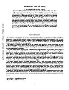
It is the inner boundary condition for the characteristic evolution which is then given by a null hypersurface version of the apparent horizon boundary condition. In the case of two black holes, the inner boundary would consist of two disjoint topological spheres, chosen so that their inner directed null normals are converging. FIG 1 provides a schematic picture of the global strategy. Two disjoint characteristic evolutions, based upon ingoing null hypersurfaces, are matched across worldtubes A and B to a Cauchy evolution of the shaded region. The interior boundary of each of these characteristic evolutions borders a region containing trapped surfaces. The outer boundary of the Cauchy region is another worldtube C, which matches to an exterior characteristic evolution based upon outgoing null hypersurfaces extending to null infinity. This strategy offers several advantages in addition to the possibility of restricting the Cauchy evolution to the region outside the black holes. Although, finding a marginally trapped surface on the ingoing null hypersurfaces remains an elliptic problem, there is a natural radial coordinate system (r, θ, φ) to facilitate its solution. However it is also possible to locate a trapped surface on the ingoing null hypersurface by a purely algebraic condition. Since this trapped surface (when it exists) lies in the region invisible to I + it can be used to replace the trapping horizon as the inner boundary. In either case, moving the black hole through the grid reduces to a 1-dimensional radial motion, leaving the angular grid intact and thus reducing the complexity of the computational masks which excise the inner region. (The angular coordinates can even rotate relative to the Cauchy coordinates in order to accommodate spinning black holes). The chief problem of this approach is that a caustic may be encountered on the ingoing null hypersurface before entering the trapped region. This is again a problem whose solution lies in choosing the right initial data and also the right geometric shape of the two-surface across which the Cauchy and characteristic evolutions are matched. There is a great deal of flexibility here because of the important feature that initial data can be posed on a null hypersurface without constraints. The strategy of matching an interior Cauchy evolution to an exterior outgoing characteristic evolution has been described [19–21] and implemented to provide a computational Cauchy outer boundary condition in various cases, ranging from 1 and 2 dimensional simulations [22–25] to 3-dimensional simulations that include I + [26,27]. A slight modification allows changing an outgoing null formalism (and its evolution code) to an ingoing one. This is briefly reviewed in Sec. II. By matching Cauchy and characteristic algorithms at both an inner and outer boundary, the ability to include I + facilitates locating the true event horizon while excising an interior trapped region. In Sec. III, we discuss the problem of locating trapped surfaces on an ingoing null hypersurface. In Sec. IV, we present an implementation of these ideas to the global evolution of spherically symmetric,

must cover a time interval of the order of several hundred M in the exterior region whereas typically a singularity forms on a time of order M in the region close to the apparent horizon. Thus a slicing which avoids the singularity for several hundred M will necessarily develop coordinate singularities. In addition, the inner boundary traced out by an apparent horizon is generically spacelike (at best lightlike). Thus if the coordinates defining the numerical grid were to remain constant in time on the boundary (“apparent horizon locking”) then the coordinate trajectories would have to be superluminal. While horizon locking works in the spherically symmetric case [2–5], it is difficult to implement in a Cartesian 3-dimensional grid. The alternative is to let the apparent horizon move through the coordinate grid. At the same time, the location of the apparent horizon must be determined by solving an elliptic equation or an equivalent extremum problem. The requirements on the grid are further complicated when the black hole is spinning. On top of all these difficulties, the computational techniques must ensure that the strong fields inside the apparent horizon boundary do not severely leak into the exterior due to finite difference approximations. Causal differencing [2] and algorithms based upon a strictly hyperbolic version of the initial value problem [18] have been proposed to avoid this. However, no 3-dimensional Cauchy code has yet been successful in evolving a Schwarzschild black hole.

C

A

B

FIG. 1. A schematic of how matching to ingoing null cones could be used with two black holes. The inner Cauchy evolution is matched at an outer world tube C to a null evolution on outgoing null cones; and at two interior world tubes A and B, to null evolutions on ingoing null cones. The evolutions on the ingoing null cones stop at the apparent horizons (dotted lines) which surround the two black holes.

It is clear that the 3-dimensional coalescence of black holes challenges the limits of computational know-how. We wish to present here a new approach for excising an interior trapped region which might provide enhanced flexibility in tackling this important problem. In this approach, we locate the interior boundary of the Cauchy evolution outside the apparent horizon. Across this inner Cauchy boundary we match to a characteristic evolution based upon an ingoing family of null hypersurfaces. 2

consistent because β contains a free integration constant which can be chosen to be complex (as long as it leads to a real metric). In order to see how this works consider the outgoing version of the null hypersurface equations [31,32]:

self gravitating scalar waves propagating in a black hole spacetime. In this case, the performance of the matching approach equals that of previous Cauchy-only schemes that have been applied to this problem [3–5,28].

1 AC BD rh h hAB,r hCD,r 16 +2πrTrr , (2.5)
B (r4 e−2β hAB U,r ),r = 2r4 r−2 β,A ,r − r2 hBC DC hAB,r

II. CAUCHY-CHARACTERISTIC MATCHING

β,r =

A. The null formalism

We introduce a unified formalism for coordinates based upon either ingoing or outgoing null hypersurfaces. Let w label these hypersurfaces, xA (A = 2, 3), be labels for the null rays and r be a surface area distance. In the resulting xα = (w, r, xA ) coordinates, the metric has the Bondi-Sachs form [29,30] ds2 = gww dw2 + 2gwr dwdr + 2gwAdwdxA +gAB dxA dxB ,

2e

(2.1)

1 AC BD rh h hAB,r hCD,r 16 +2πrTrr , (2.8)
2 BC −2 4 −2β B 4 −(r e hAB U,r ),r = 2r r β,A ,r − r h DC hAB,r β,r =

(2.2)

+16πr2 TrA (2.9) −2β A A −2e V,r = R − 2D DA β − 2D βDA β −r−2 e−2β DA (r4 U A ),r 1 A B − r4 e−4β hAB U,r U,r 2 +8πr2 (T − g AB TAB ).

(2.3)

in the outgoing form of the metric. The substitution (2.3) can also be used in the curved space case to switch from outgoing to ingoing coordinates, in which case it is equivalent to an imaginary shift in the integration constant for the Einstein equation determining β (see equation (2.5) below). This leads to the ingoing version of the metric   V ds2 = e2β + r2 hAB U A U B dv 2 + 2e2β dvdr r −2r2 hAB U B dvdxA + r2 hAB dxA dxB .

(2.7)

where DA is the covariant derivative and R the curvature scalar of the 2-metric hAB . The β-equation (2.5) allows the substitution (2.3) to be regarded as a change in integration constant. Then carrying out this substitution in equations (2.5)-(2.7) leads to the ingoing version of the null hypersurface equations:

A where hAB hBC = δC . This yields the standard outgoing null coordinate version of the Minkowski metric by setting β = U A = V − r = hAB − qAB = 0. In the ingoing case, writing w = v, the only component of the Minkowski metric which differs is gvr = −gur . This can be effected by the substitution

β → β + iπ/2

+16πr2 TrA (2.6) V,r = R − 2DA DA β − 2DA βDA β +r−2 e−2β DA (r4 U A ),r 1 A B − r4 e−4β hAB U,r U,r 2 +8πr2 (T − g AB TAB ),

where det(gAB ) = r2 det(qAB ) = r2 q, with qAB a unit sphere metric. In the outgoing case, writing w = u, it is convenient to express the metric variables in the form   V ds2 = − e2β − r2 hAB U A U B du2 − 2e2β dudr r − 2r2 hAB U B dudxA + r2 hAB dxA dxB ,

−2β

(2.10)

This formal substitution also applies to the dynamical equations and provides a simple means to switch between evolution algorithms based upon ingoing and outgoing null cones. As we have already noted, although the same coordinate labels r and xA are used for notational simplicity in both the outgoing metric (2.2) and the ingoing metric (2.4), they represent different fields. An exception occurs for spherical symmetry where the the surface area coordinate r can be defined uniquely in terms of the same 2-spheres of symmetry used in both the ingoing and the outgoing coordinates. In this case, the spacelike or timelike character of the r = const hypersurfaces is consistent under the substitution (2.3) because the change involved in going from (2.7) to (2.10) implies that V changes sign in switching from outgoing to ingoing coordinates. As a result we obtain a consistent value for g αβ r,α r,β = ±e−2β V /r, with the + (−) sign holding for outgoing (ingoing) coordinates.

(2.4)

Of course, at a given space-time point the values of the coordinates r and xA and the metric quantities β, U A , V and hAB are not the same in the ingoing and outgoing cases; but since we do not consider transformations between outgoing and ingoing coordinates there is no need to introduce any special notation to distinguish between them. This same substitution also provides a simple switch from the outgoing to the ingoing version of Einstein equations Gαβ = 8πTαβ written in null coordinates. This is 3

null hypersurfaces vt on an inner boundary Q whose location is determined by a trapping condition, as discussed below. This inner boundary plays a role analogous to an apparent horizon inner boundary in a pure Cauchy evolution. The region inside Q is causally disjoint from the domain of dependence which is evolved from the initial data. In the implementation of this strategy in the model spherically symmetric problem of Sec. IV, we describe in detail how data is passed back and forth across W to supply an outer boundary value for the null evolution and an inner boundary value for the Cauchy evolution. In the remainder of this section, we discuss how some of the key underlying issues might be handled in the absence of symmetry. In order to ensure that an inner trapping boundary exists it is necessary to choose initial data which guarantees black hole formation. Such data can be obtained from initial Cauchy data on t0 for a black hole. However, rather than extending the Cauchy hypersurface inward to the apparent horizon it could instead be truncated at an initial matching surface S0 located sufficiently far outside the apparent horizon to avoid computational problems with the Cauchy evolution. The initial Cauchy data would then be extended into the interior of S0 as null data on v0 until a trapping boundary is reached. Two ingredients are essential in order to arrange this. First, S0 must be chosen to be convex, in the sense that its outward null normals uniformly diverge and its inner null normals uniformly converge. Given any physically reasonable matter source, the focusing theorem then guarantees that the null hypersurface v0 emanating inward from S0 continues to converge until reaching a caustic. Second, initial null data must be found which leads to trapped surfaces on v0 before such a caustic is encountered. The existence of trapped surfaces depends upon the divergence of the outward normals to slices of v0 . Given the appropriate choice of S0 the existence of such null data is guaranteed by the evolution of the extended Cauchy problem. However, it is not necessary to actually carry out such a Cauchy evolution to determine this null data. It is the data on S0 which is most critical in determining whether a black hole can form. This can be phrased in terms of the trapping gravity of S0 , introduced below. In the spherically symmetric Einstein-Klein-Gordon model (see Sec. IV), if S0 has sufficient trapping gravity to form a trapped surface on v0 in the absence of scalar waves crossing v0 then a trapped surface also forms in the presence of scalar waves. In the absence of symmetry, this suggests that given appropriate initial Cauchy data for horizon formation that the simplest and perhaps physically most relevant initial null data for a black hole would correspond to no gravitational waves crossing v0 . The initial null data on v0 can be posed freely, i.e. it is not subject to any elliptic or algebraic constraints other than continuity requirements with the Cauchy data at S0 . In the vacuum case, the absence of gravitational waves in the null data has a natural (although approximate) formulation in terms of setting the ingoing null component

In the absence of spherical symmetry, the surface area coordinate r used in the Bondi-Sachs formalism has a gauge ambiguity associated with the changes in ray labels xA → y A (xB ), under which it transforms as a scalar density. On any null hypersurface with a preferred compact spacelike slice S0 , this coordinate freedom in r may be fixed by requiring that r = const on S0 . This then determines a unique r = const foliation on either the ingoing or outgoing null hypersurface emanating from S0 . B. Matching

Cauchy-characteristic matching can be used to replace artificial boundary conditions which are otherwise necessary at the outer boundary of a finite Cauchy domain. The exterior characteristic evolution can then be extended to null infinity to form a globally well-posed initial value problem. In tests of nonlinear 3-dimensional scalar waves, Cauchy-characteristic matching dramatically outperforms the best available artificial boundary condition both in accuracy and computational efficiency [26,27]. We now describe how this matching strategy can be used at the inner boundary of a Cauchy evolution which is joined to an ingoing null evolution. On the initial Cauchy hypersurface, denoted by time t0 , let S0 be a (topological) 2-sphere forming the inner boundary of the region being evolved by Cauchy evolution. Let W represent the future evolution of S0 under the flow of the vector field ta = αna + β a , where na is the unit vector field normal to the Cauchy hypersurfaces t = const and α and β a are the lapse and shift. Given the initial Cauchy data on t0 , boundary data must be given on the world tube W in order to determine its future evolution. The Cauchy hypersurfaces foliate this world tube into spheres St . The boundary data is obtained by matching across W to an interior null evolution based upon the null hypersurfaces v = const emanating inward from from the spheres St . The evolutions are synchronized by setting v = t on W. W

Q

v0 t0

v0 t0

FIG. 2. The shaded region is the domain of dependence of initial data which is given on a Cauchy slice t0 and an ingoing null slice v0 . Q is the apparent horizon. W is the matching world tube.

The combination of initial null data on v0 and initial Cauchy data on t0 determine the future evolution in their combined domain of dependence as illustrated in FIG 2. In order to avoid dealing with caustics we terminate the

4

of the Weyl tensor to zero on v0 . Key to the success of this approach is the proper trapping behavior, i.e. the convergence of both sets of null vectors normal to a set of slices of v0 located between the caustics and the matching boundary. By construction, the ingoing null hypersurface N0 , given by v = v0 , is converging along all rays xA leaving the initial slice S0 coordinatized by r = R0 . (Here (v, r, xA ) are ingoing null coordinates.) In order to investigate the trapping of N0 we must determine the divergence of slices S of N0 defined by r = R(xA ). Let nα be tangent to the generators of N0 , with normalization nα = −gvr v,α . Then α nα v,α = nα xA ,α = 0 and n r,α = −1. Let lα be the outgoing normal to S, normalized by nα lα = −1. Then lα = −lv,α + r,α − R,A xA ,α

III. TRAPPING

A slice of N0 is trapped if Θl < 0. In terms of the ingoing Bondi metric variables defined in (2.4), equation (2.16) gives 1 √ r2 e2β Θl = − V − √ [ q(e2β hAB R,B − r2 U A )],A 2 q A − r(r−1 e2β hAB ),r R,A R,B + r2 R,A U,r . (3.1)

Setting Θl = 0 in equation (3.1) gives a 2-dimensional Laplace equation for the function R(xA ) which locates a marginally trapped surface A. Such a surface lies on a trapping horizon and is (a component of) the apparent horizon of any Cauchy hypersurface which contains it. For a marginal surface to lie on an outer trapping horizon its trapping gravity, defined as [16] r 1 κ = − Ln Θl , (3.2) 8

(2.11)

where l=

1 gvr (g rr − 2g rAR,A + g AB R,A R,B ). 2

(2.12)

Its contravariant components are v

l =g

lr =

vr

1 rr 1 AB g − g R,A R,B 2 2

must be real and positive, so that κ ≥ 0. The trapping gravity generalizes the concept of the surface gravity of an event horizon to trapping horizons. In our coordinate system, nα ∂α = −∂r . Thus if the surface r = R(xA ) is marginally trapped then positive trapping gravity implies that the surface r = R(xA ) − ∆r is trapped for small ∆r. We use equation (3.2) to generalize the definition of trapping gravity to an arbitrary slice of a inwardly converging null hypersurface. Then slices of positive trapping gravity tend toward trapping as r decreases. However, in general, there seems to be no purely local criterion which guarantees the existence of a trapped surface before encountering a caustic as r → 0. In the special case of a spherically symmetric slice of a spherically symmetric null cone, the Laplace equation for a marginally trapped slice reduces to the algebraic condition that V = 0, which is satisfied where the r = const hypersurface becomes null. The vacuum Schwarzschild metric in ingoing null coordinates (which are equivalent to ingoing Eddington-Finkelstein (IEF) coordinates) is given by β = 0, V = −(r−2M ), U A = 0 and hAB = qAB . In this case, V = 0 determines the location of the event horizon (which coincides with the apparent horizon) and the surface gravity reduces to κ = (4M )−1 . In the nonvacuum spherically symmetric case, V = 0 determines the apparent horizon. In the absence of spherical symmetry, Θl vanishes on a slice of the form R = const at points for which Q = 0, where

(2.13)

(2.14)

and lA = g rA − g AB R,B .

(2.15)

Let γβα = gβα + nα lβ + lα nβ be the projection tensor into the tangent space of S and define γ αβ and γαβ by raising and lowering indices with gαβ . Its contravariant components are γ αv = 0, γ AB = g AB , γ rA = g AB R,B and γ rr = g AB R,A R,B ; and its covariant components are γαr = 0, γAB = gAB , γvA = gvr R,A + gvA and γvv = g AB (gvr R,A + gvA )(gvr R,B + gvB ). The outward divergence of S is given by Θl = 2γ αβ ∇α lβ . (The conventions are chosen so that Θ = 2/r for a r = const slice of an outgoing null cone in Minkowski space.) Then a straightforward calculation yields 1 1 g vr √ Θl = g rr − √ [ qg AB (gvr R,B + gvB )],A 2 r q g vr − (rgvr g AB ),r R,A R,B r −g vr R,B (g AB gvA ),r , (2.16)

r2 √ Q = −V + √ ( qU A ),A . q

which is to be evaluated on S after the derivatives are taken. The divergence of the generators tangent to N0 is given by Θn = γ αβ ∇α nβ . Then Θn = −2/r so that N0 is converging in accord with our construction.

(3.3)

We will refer to the largest r = const slice of N0 on which Q ≤ 0 as a “Q-boundary” Q, relative to S0 . (S0 enters here because it provides the reference for r = const slices). Such a slice is everywhere trapped or marginally 5

Our purpose here is to present a spherically symmetric model demonstrating the feasibility of a stable global algorithm based upon three regions which cover the spacetime exterior to a single black hole. FIG 3 illustrates 1-dimensional radial geometry. The innermost region is evolved using an ingoing null algorithm whose inner boundary Q lies at the apparent horizon and whose outer boundary R0 lies outside the black hole at the inner boundary of a region evolved by a Cauchy algorithm. Data is passed between these regions using a matching procedure which is detailed below. The outer boundary R1 of the Cauchy region is handled by matching to an outgoing null evolution. The details of the outgoing null algorithm [33] and of the Cauchy evolution [5] are not discussed since they have been presented elsewhere. We will discuss the matching conditions since they differ from those used previously [25] due to different choices of gauge conditions. We will also present the field equations since they are important for understanding the matching procedure. The Cauchy evolution is carried out in IEF coordinates. The metric in this coordinate system is   ˜ t˜d˜ r+a ˜2 d˜ r2 + r˜2 dΩ2 . a2 βd ds2 = a ˜2 2β˜ − 1 dt˜2 + 2˜

trapped so that the Q-boundary provides a simple algebraic procedure for locating an inner boundary inside an event horizon. A Q-boundary, when it exists, will always lie inside (smaller r) or tangent to the trapping horizon. Let r = RQ describe the Q-boundary and let Rmin (Rmax ) be the smallest (largest) value of r on the trapping horizon. Then on the trapping horizon R,A = 0 at Rmin and Rmax so that equation (2.16) implies Q ≥ 0 at Rmin (and Q ≤ 0 at Rmax ). Consequently, RQ ≤ Rmin , with equality holding only when D2 R = 0 at Rmin . There are thus two possible strategies for positioning an inner boundary, both of which ensure that the ignored portion of spacetime cannot causally effect the exterior spacetime: (I) Use the trapping horizon, in which case the 2D elliptic equation (2.16) must be solved on a sphere in order to determine its location; or (II) use the Q-boundary which is determined by a simple algebraic condition. Strategy (I) is similar to approaches used to locate an apparent horizon on a Cauchy hypersurface. The advantage in the null cone case is that there is a natural radial coordinate defined by the coordinate system to reduce the elliptic problem to 2 angular dimensions and to define a mask for moving the excised region through the computational grid. Strategy (II) carries no essential computational burden since the quantities V and U are obtained by means of an inward radial integral as part of the evolution scheme. One merely stops the integration when the inequality defining the Q-boundary is satisfied. Thus strategy (II) is preferable unless either caustics or singularities appear before reaching the Q-boundary. It is easy to choose black hole initial data so that the Qboundary and trapping horizon agree at the beginning of the evolution but whether the Q-boundary will move too far inward to be useful is a critical question which would depend upon choices of lapse, shift and the geometry of the matching world tube. Further research is necessary to decide if strategy (II) is viable on geometric grounds in a highly asymmetric spacetime.

(4.1)

The set of equations used in the evolution are K θ′θ +

β˜ =

v 0

(4.2)

(4.3)

(4.4)

 
˜ θ′ + a K˙θ θ = βK ˜ 1 − β˜ K θ θ K r r + 2K θ θ θ   β˜′ 1 1 − β˜ + , a ˜− + 2 (4.5) r˜ a ˜ a ˜r˜

Q

R

r˜a ˜K θ θ , 1 + r˜a ˜K θ θ

   ′ ˜β˜ , a ˜˙ = −˜ a2 1 − β˜ K r r + a

IV. COLLAPSE OF A SPHERICALLY SYMMETRIC SCALAR WAVE

R 0

4πΦΠ Kθθ − Krr − = 0, r˜ a ˜

   ′ ˜ + 1 − β˜ Π , Φ˙ = βΦ

1

(4.6)

h    i′ ˜ + 1 − β˜ Φ ˙ = 1 r˜2 βΠ , Π 2 r˜

(4.7)

1  ˙ ˜ ′ φ − βφ . 1 − β˜

(4.8)

where the over-dot represents partial with respect to t˜, prime denotes partial with respect to r˜ and the scalar field variables are defined by

u0

t0

FIG. 3. This figure shows the two matching world tubes and the three coordinate patches.

Φ ≡ φ′ 6

Π≡

i h φ = A˜ r exp − (˜ r − c)d /σ d , " # d−1 1 d (˜ r − c) Φ=φ , − r˜ σd   d−1 ˜ 2 − β d (˜ r − c) , − Π = φ  σd r˜ 1 − β˜

The outgoing-null metric is ds2 = −e2β

V 2 du − 2e2β dudr + r2 dΩ2 , r

(4.9)

The outgoing hypersurface equations (2.5) - (2.7) reduce to β,r =

2πrφ2,r , 2β

V,r = e ,

(4.10) (4.11)

1 (rV φ,r ),r . r

V 2 dv + 2e2β dvdr + r2 dΩ2 , r

B. Matching conditions

Since the IEF coordinate system is based on ingoing null cones, it is possible to construct a simple coordinate transformation which maps the IEF Cauchy metric to the ingoing null metric, namely

(4.13)

t˜ = v − r,

an independent set of equations are the hypersurface equations β,r = 2πrφ2,r , 2β

V,r = −e , 1 (rV φ,r ),r . r

(4.14) (4.15)

2β˜ − 1 1 − β˜ V +r β˜ = V + 2r p a ˜ = eβ V /r + 2.

V =r (4.16)

Given data for φ on N0 and on the world tube R0 , defined by r = R0 , and integration constants for β and V on R0 evolution proceeds to null hypersurfaces Nv , defined by v = const, by an inward radial march along the null rays emanating inward from R0 .

(4.23)

(4.25) (4.26) (4.27)

The extrinsic curvature components can be found using only the Cauchy metric,

The initial data consists of a Schwarzschild black hole of mass M which is well separated from a Gaussian pulse of (mostly) ingoing scalar radiation. Initially there is no scalar field present on the ingoing-null patch, so the initial data there is simply

β˜   r˜a ˜ 1 − β˜   1 a ˜′ a ˜˙  β˜′ + β˜ − =  . ˜a a ˜ a ˜ 1 − β˜

Kθθ =

(4.28)

Krr

(4.29)

A. Initial data

φ = 0, β = 0, V = 2M − r.

r˜ = r.

This results in the following transformations between the two metrics. i h  (4.24) β = 1/2 log a ˜2 1 − β˜

and the scalar wave equation 2(rφ),rv =

(4.22)

(4.12)

An ingoing null evolution algorithm can be obtained from the outgoing algorithm by the procedure described in Sec. II. Given the ingoing null metric ds2 = e2β

(4.21)

where A, c, d, and σ are scalars representing the pulse’s amplitude, center, shape, and width, respectively. The geometric variables are initialized using an iterative procedure, as detailed in [5].

with U A = 0 and hAB = qAB , and the outgoing version of the scalar wave equation is 2(rφ),ru =

(4.20)

Note that these transformation equations are valid everywhere in the spacetime, not just at the world tube. The matching conditions at the outer world tube are more complicated. Both the Cauchy and characteristic systems share the same surface area coordinate r but there is no universal transformation between their corresponding time coordinates. However, we can construct a coordinate transformation which is valid everywhere on the world tube. To do this, we start with a general, differential coordinate transformation, whose unknown function F is to be determined from the matching conditions:

(4.17) (4.18) (4.19)

Similarly, initially there is no scalar field on the outgoing-null patch, so we have φ = 0. The values for β and V are determined by matching to the Cauchy data at the world tube (see below) and integrating the hypersurface equations (4.14) and (4.15). In the Cauchy region, the scalar field is given by

d¯ u = F (t˜)dt˜ − d˜ r, 7

dr = d˜ r.

(4.30)

To keep the notation simpler, we will write the Cauchy metric as ds2 = g00 dt˜2 + 2g01 dt˜d˜ r + g11 d˜ r2 + r˜2 dΩ2 . Inverting (4.30) and substituting, we get   1 1 1 2 2 udr u +2 g01 + 2 g00 d¯ ds = g00 2 d¯ F F F   2 1 + g11 + g01 + 2 g00 dr2 + r2 dΩ2 . F F

R

(4.31)

1 N -2 i

n n-1 N -1 i N i FIG. 4. This diagram shows the finite difference grids around the inner world tube. The squares represent the Cauchy grid, while the circles are the null grid. The diagonal lines are the ingoing null cones, and the vertical line R0 is the inner world tube. The innermost points of the Cauchy grid lie on the world tube, while the null grid extends outside the world tube. Notice that the grids align in space and time.

(4.34)

Upon substitution of the IEF metric functions, this determines that ˜ F = 1 − 2β. The matching conditions are then i h  β = 1/2 log a ˜2 1 − β˜ 1 − 2β˜ 1 − β˜ V −r β˜ = V − 2r p a ˜ = eβ 2 − V /r.

V =r

3

n+1

(4.32)

The condition that the r-direction be null implies that 2 1 g01 + 2 g00 = 0. F F

2

n+2

On the world tube, we require u = t˜, sothat du = dt˜. Thus, we set du = d¯ u/F . For the metric, we get   1 2 2 ds = g00 du + 2 g01 + g00 dudr F   1 2 + g11 + g01 + 2 g00 dr2 + r2 dΩ2 . (4.33) F F

g11 +

0

In addition to the spatial discretization, each function needs two or more time levels. While both the Cauchy and null evolution schemes use only two time levels, we keep an extra level in each to facilitate the matching. FIG 4 shows how the finite difference grids match at the inner world tube. The two grids are aligned in both r and t˜. This means no interpolations are necessary. The world tube is at i = 1 on the Cauchy grid and i = Ni − 1 on the ingoing null grid. The Cauchy variables need boundary values on time level n + 1 at i = 1. The metric values come from the null variables at level n + 1, with i = Ni − 1, using the transformation equations (4.26) and (4.27). These relations are algebraic and straightforward to implement. Boundary values for the extrinsic curvature components come from equations (4.28) and (4.29). K θ θ is computed algebraically and K r r is computed using second-order, centered-in-time, forward-inspace derivatives in the Cauchy grid. The transformation of the scalar field requires transforming derivatives between the two coordinate patches. At the world tube, the relationships among the derivatives are

(4.35)

(4.36) (4.37) (4.38) (4.39)

C. Finite difference implementation

As is typical with finite difference calculations, the continuum functions are discretized spatially and placed on grids with N points. In our case we have three regions. The inner-null variables are placed on grids with Ni points, the Cauchy variables on grids with Nc points, and the outer-null variables on grids with No points. On each grid, the spatial index i runs from 1 to Ni , Nc or No , respectively, with 1 representing the smallest r value.

∂r = ∂r˜ − ∂t ∂r˜ = ∂r + ∂v ∂v = ∂t .

(4.40) (4.41) (4.42)

These lead to the following equations for Φ and Π: Φn+1 = 1

n+2 n+1 n+1 n g n+1 1 gNi −1 − gN 1 gNi − gNi −2 i −1 + − Ni2−1 r˜1 2dv r˜1 2dr r˜1

(4.43) 8

to get an evolution equation for φ at the world tube. We then set Φ and Π using their definitions (4.8) and backward second-order derivatives. The boundary values for the null variables must be interpolated in time using the Cauchy variables at n and n − 1. Given values for a function f at time levels n and n − 1, we can get its value f s at the beginning of the null cone using ! dr 1 fs = fn 3 − n+2 dt 1 − 2β˜N c −1 ! dr 1 n−1 . (4.47) −2 + +f dt 1 − 2β˜n+2

and Πn+1 = 1

1 1 − β˜1n+1

!

n+2 n 1 gNi −1 − gN i −1 . − β˜1n+1 Φn+1 1 r˜1 2dv

(4.44) The null variables need boundary values at n + 2, i = Ni . The metric values come from the Cauchy variables at level n, with i = 2, using (4.24) and (4.25). The evolution equation for g at the world tube is " ! β˜2n + β˜2n−1 Πn2 + Π2n−1 n+2 n+2 1− gNi = gNi + rNi dv 2 2 # β˜n + β˜2n−1 Φn2 + Φ2n−1 + 2 . (4.45) 2 2

Nc −1

Notice that this expression requires a value for β˜ at level n+ 2, something that won’t be known until the next time step. We have found it sufficient to extrapolate from the previous time levels using n+2 n+1 n−1 n β˜N = 3β˜N − 3β˜N + β˜N . c −1 c −1 c −1 c −1

N -2 c

Nc-1

Thus, to get values for β and V we use the matching conditions (4.36) and (4.37) along with the above interpolation. For the scalar field, we interpolate the value of g from the Cauchy grid, using g = rφ. The apparent horizon is found on the ingoing null cones using the apparent horizon equation which reduces simply to V = 0. When the scalar field passes into the black hole, the horizon grows outward and we simply stop evolving the grid points that are now inside.

Nc

n+2

3

n+1 n

(4.48)

2

n-1 D. Performance

R

1

To evaluate the performance of this approach, we compare it to a second order accurate, purely Cauchy evolution in IEF coordinates, as presented in [5]. For the comparison shown here, we place the outer boundary of the Cauchy evolution at r = 62M and evolve to t = 40M to prevent any outer boundary effects from influencing the comparison. The scalar field pulse is centered at r = 22M and has a mass of 0.5M . FIG 6 shows the mutual convergence between the Cauchy variables in the two codes. This demonstrates that the two programs are solving the same problem, and provides evidence that the matching approach generates the correct spacetime.

1 FIG. 5. This diagram shows the finite difference grids around the outer world tube. The squares represent the Cauchy grid, while the circles are the null grid. The diagonal curves are the outgoing null cones, and the vertical line R1 is the outer world tube. The outermost points of the Cauchy grid lie on the world tube, while the null grid extends inside the world tube. Notice that the the grids align in time only on the world tube, but in space at the world tube and just inside.

The situation at the outer world tube is shown in FIG 5. Here, the grids align in space at two values of r but in time only at the world tube. The Cauchy metric boundary values at i = Nc come directly from the null variables at i = 2 using the transformation equations (4.38) and (4.39). Since the grids don’t align in time as they do at the inner world tube, we use a different procedure for the scalar field boundary values. We use the derivative transformation ∂r =

1 ∂t + ∂r˜ 1 − 2β˜

(4.46)

9

6

the matching may be tricky, especially in higher dimensions. Whether it is easier than implementing Cauchy differencing near the horizon remains to be seen. Also, using the ingoing null formulation, we have achieved the stable evolution of a Schwarzschild black hole in 3-dimensions (the details will be presented elsewhere) and are working on rotating and moving black holes. Long term stable evolution of a 3D black hole has yet to be demonstrated with a Cauchy evolution.

Convergence Factor

α 5

∼ β

4

Κ

3

Φ

2

φ

θ θ

Π 1

ACKNOWLEDGMENTS

0 0

5

10

15

20 t

25

30

35

40

FIG. 6. This plot shows the mutual convergence of the Cauchy variables from the matching evolution and the pure Cauchy evolution. The evolutions are for a strong, ingoing scalar pulse (0.5M ) outside a black hole. A convergence factor near four indicates second order convergence, while one near two indicates first order convergence.

This work has been supported by NSF PHY 9510895 to the University of Pittsburgh and by the Binary Black Hole Grand Challenge Alliance, NSF PHY/ASC 9318152 (ARPA supplemented). Computer time for this project has been provided by the Pittsburgh Supercomputing Center under grant PHY860023P. We thank R. A. Isaacson for helpful comments on the manuscript.

The reason that the convergence rate appears to drop to first order when the scalar field hits the horizon is an artifact arising from the motion of the horizon. As mass falls into the hole, there is a critical amount which causes the horizon to move out by one grid point. If at the coarsest resolution the horizon moves a distance dr then on the next finer grid it only moves by dr/2, and so on. Thus, at different resolutions, the black holes have slightly different locations. The resulting shift in the location of the inner boundary causes convergence between successively finer numerical solutions to drop from second order to first order. This is an unavoidable diagnostic effect due to the comparison of numerical solutions. We believe that the numerical solution would converge at second order to an exact solution of the physical problem. No exact solutions are known to use for a check of this, but for a weak scalar field the horizon does not move and we do measure second order convergence throughout the evolution. Further, we see the same convergence order drop for strong fields in Cauchy-only or null-only evolutions, and thus are certain it is not due to the matching procedure.

[1] [2] [3] [4] [5] [6] [7] [8] [9] [10] [11] [12]

[13]

V. CONCLUSIONS

Our work shows that the matching approach provides as good a solution to the black hole excision problem in spherical symmetry as previous treatments [3–5,28]. It also has some advantages over the pure Cauchy approach, namely, it is computationally more efficient (fewer variables), and is much easier to implement. We achieved a stable evolution simply by transforming the outgoing-null evolution scheme to work on ingoing null cones, and implementing it. Achieving stability with a purely Cauchy scheme in the region of the apparent horizon is trickier, involving much trial and error in choosing difference schemes. It should be noted, however, that implementing

[14] [15] [16] [17]

[18] [19] [20] [21]

10

J. Thornburg, Class. Quantum Grav. 4, 1119 (1987). E. Seidel and W. Suen., Phys. Rev. Lett. 69, 1845 (1992). M. A. Scheel et al., Phys. Rev. D 51, 4208 (1995). M. A. Scheel et al., Phys. Rev. D 51, 4236 (1995). R. L. Marsa and M. W. Choptuik, Phys. Rev. D 54, 4929 (1996). J. Thornburg, Phys. Rev. D 54, 4899 (1996) G. Cook and J. W. York, Phys. Rev. D 41, 1077 (1990). K. P. Tod, Class. Quantum Grav. 8, L115 (1991). T. Nakamura, Y. Kojima and K. Oohara, Phys. Lett. 106A, 235 (1984). A. J. Kemball and N. T. Bishop, Class. Quantum Grav. 8, 1361 (1991). M. F. Huq, S. A. Klasky, M. W. Choptuik and R. A. Matzner, (unpublished). P. Anninos, K. Camarda, J. Libson, J. Mass´ o, E. Seidel and W. Suen, “Finding Apparent Horizons in Dynamic 3D Numerical Spacetimes”, gr-qc 9609059. T. W. Baumgarte, G. B. Cook, M. A. Scheel, S. L. Shapiro and S. A. Teukolsky, Phys. Rev. D 54, 4849 (1996). Robert M. Wald, General Relativity. (1984). Robert M. Wald and Vivek Iyer, Phys. Rev. D 44, R3719 (1991). S. A. Hayward, Phys. Rev. D 49 6467 (1994). G. B. Cook, M. W. Choptuik, M. R. Dubal, S. Klasky, R. A. Matzner and S. R. Oliveira, Phys. Rev. D, 47, 1471 (1993). A. Abrahams, A. Anderson, Y. Choquet-Bruhat and J. W. York, Phys. Rev. Lett. 75, 3377 (1995) J. Anderson, J. Comput. Phys. 75, 288 (1988). N. T. Bishop, in Approaches to Numerical Relativity (1992). N. T. Bishop, Class. Quantum Grav. 10, 333 (1993).

[22] C.J.S. Clarke and R.A. d’Inverno, Class. Quantum Grav. 11, 1463 (1994). [23] C.J.S. Clarke and R.A. d’Inverno, and J.A. Vickers, Phys. Rev. D 52, 6863 (1995). [24] M. R. Dubal, A. d’Inverno and C.J.S. Clarke, Phys. Rev. D 52, 6868 (1995) [25] R. G´ omez, P. Laguna, P. Papadopoulos and J. Winicour., Phys. Rev. D 54, 4719 (1996). [26] N. T. Bishop et al., Phys. Rev. Lett. 76, 4303 (1996). [27] N. T. Bishop et al., submitted to J. Comput. Phys. (1996). [28] P. Anninos et. al., Phys. Rev. D 51 5562 (1995). [29] H. Bondi, et al., Proc. R. Soc. Ser. A 269, 21 (1962). [30] R. Sachs, Proc. R. Soc. Ser. A 270, 103 (1962). [31] J. Winicour, J. Math. Phys. 24, 1193 (1983). [32] J. Winicour, J. Math. Phys. 25, 2506 (1984). [33] R. G´ omez and J. Winicour, J. Math. Phys. 33, 1445 (1992).

11