BUREAU OF RECLAMATION AUTOMATED MODIFIED EINSTEIN PROCEDURE (BORAMEP) PROGRAM FOR COMPUTING TOTAL SEDIMENT LOAD Christopher L. Holmquist-Johnson, Hydraulic Engineer, Sedimentation and River Hydraulics Group, Technical Service Center, Bureau of Reclamation, Denver, CO,
[email protected] David Raff PhD, PE, Hydraulic Engineer, Flood Hydrology Group, Technical Service Center, Bureau of Reclamation, Denver, CO,
[email protected] INTRODUCTION Developing a reliable and consistent method of computing total sediment discharge within a river is one of the most important practical objectives of research in fluvial processes (Burkham and Dawdy, 1980). Current techniques for suspended sediment collection do not allow sampling throughout the entire depth of flow and therefore the concentration and particle size distribution in only part of the flow can be determined from the suspended-sediment samples. The unsampled flow near the stream bed normally contains higher concentrations and coarser particle-size distributions than the flow in the sampled zone. Thus, the concentration of suspended-sediment samples is usually lower than the suspended-sediment concentration for the entire depth, and the particle sizes of the samples are usually smaller that the particle sizes for the entire depth. In 1950, Einstein presented a procedure for computing the total discharge of sediment of sizes found in appreciable quantities in the stream bed for a long reach of a stream channel. However, acquiring the data required by Einstein’s procedure was very labor intensive and time consuming. In 1955, Colby and Hembree presented a modified version of Einstein’s procedure (MEP) that used data from a single cross section to calculate the total sediment discharge for a particular reach. The MEP is considered an improvement over the original Einstein method because it is simpler in computation and it uses parameters more readily available from actual stream measurements. The modified method, however, requires a great deal of experience and judgment to obtain reliable results and often times the results are not easily replicated by multiple users. Computations are made for several ranges of particle sizes and involve many variables resulting in a very complex process of computing total sediment load. As a result, a more simplified and automated method of computing total sediment discharge for a given reach that can be reproduced by numerous users is of great interest. The primary objective of this manuscript is to present a reliable and readily automated algorithm for computing total sediment load using Reclamations version of the MEP procedure as described in Reclamations 1955 and 1966 publications. The algorithm has been developed and deployed through a computer program that is applicable to a wide range of flow and sediment conditions and provides information to identify areas where additional research might be needed. This paper describes the Bureau of Reclamation Automated Modified Einstein Procedure (BORAMEP) program and procedures (Holmquist-Johnson and Raff, 2005) that were used to automate the process of calculating total sediment load using the MEP procedure.
METHODS Modified Einstein Equations and Procedure The following presents the basic steps required during the calculation of total load using the Modified Einstein Procedure with additional information provided in areas where calculations have been automated. 1) Compute the measured suspended load. Qs = 0.0027 Q Conc (tons / day )
(1)
2) Compute the product of the hydraulic radius and friction slope assuming x = 1. 2a) First, compute the value of ( RS f using Colby and Hembree ‘s (1955) equation E.
( RS f =
Vavg ⎡ h 32.63 log ⎢12.27 ks ⎣
⎤ x⎥ ⎦
(2)
2b) Compute the shear velocity.
U * = g ( RS f )
(3)
2c) Compute the laminar sublayer thickness δ. 11.6v δ= U*
(4)
2d) Recheck x to make sure that the initial guess of x = 1 is valid. Step 2 becomes an iterative process utilizing a newly fit equation to Colby and Hembree ‘s k (1955) Plate 3 describing the relationship between x and s . The equation presented in Figure 1
δ
is considered valid for 0.2 ≤
ks
δ
≤ 40 .
3) Compute the value of P.
⎡ hx ⎤ P = 2.303 log ⎢30.2 ⎥ ks ⎦ ⎣ 4) Compute the fraction of the flow depth not sampled (A’). d A' = n ds
(5)
(6)
5) Compute the sediment discharge Q’s through the sampled zone. This is calculated using a percentage of the flow sampled determined from the appropriate equation for the value of A’ and P. Equations 8 – 11 were calculated by fitting equations to Colby and Hembree ‘s (1955) Plate 4 and are used to automate the calculations of % flow sampled. Qs' total = Qs * % flow sampled (7)
x=
1.8
1 .5
2
⎛k ⎞ ⎛k ⎞ ⎛k ⎞ + 2.88.37⎜ s ⎟ − 195.25⎜ s ⎟ + 57.6⎜ s ⎟ ⎝δ ⎠ ⎝δ ⎠ ⎝δ ⎠ 1 .5 2 2 .5 ks ks ⎛ ks ⎞ ⎛ ks ⎞ ⎛ ks ⎞ − 139.12 + 237.35⎜ ⎟ − 181⎜ ⎟ + 56.7⎜ ⎟ 1 + 33.96 δ δ ⎝δ ⎠ ⎝δ ⎠ ⎝δ ⎠
− 9.95 + 75.30
ks
δ
− 201.73
ks
2 .5
δ
( Plate#3)
1.6
1.4 Smooth Wall x 1.2
Rough Wall
1
0.8
0.6 0.1
1
10
100
ks/δ
Figure 1 – Correction x in the logarithmic friction formula in terms of ks/δ. For P=4, % flow sampled= 100 − 2941.79 A' 2 +265357.48 A' 4 +64219.08 A' 6 −325482.24 A'8 1 − 29.38 A' 2 +2621.48 A' 4 +5407.23 A' 6 +157.44 A'8 +1272.32 A'10 For P=8, % flow sampled= 100 + 30991.16 A' 2 +21184.18 A' 4 +211800.14 A' 6 −263775.36 A'8 1 + 325.87 A' 2 +1201.21A' 4 +1872.11A' 6 +5759.38 A'8 −2976.45 A'10 For P=11, % flow sampled= 100.19 + 31425.83 A' 2 −54359.86 A' 4 +1566703.2 A' 6 −1543898.1A'8 1 + 336.12 A' 2 +444.29 A' 4 +15662.05 A' 6 +18936.5 A'8 −5820.32 A'10 For P=14, % flow sampled= 100.31 + 45744.98 A' 2 +103307.39 A' 4 +635604.51A' 6 −784215.44 A'8 1 + 485 A' 2 +2934.57 A' 4 +7640.27 A' 6 +11737.99 A'8 −3015.81A'10
(8)
(9)
(10)
(11)
6) Compute the bed-load for each size fraction. 6a) The first step in computing the bedload is to calculate the shear intensity (ψ) for all particle sizes in the analysis by using the minimum of the following two equations, where di is the geometric mean for each size class: ⎛ d 35 ⎝ RS f
ψ = 1.65⎜⎜
⎛ ⎞ ⎟ or 0.66⎜ d i ⎜ RS ⎟ ⎝ f ⎠
⎞ ⎟ ⎟ ⎠
(12)
6b) Colby and Hembree ‘s (1955) Plate#2 was used to determine the intensity of bed-load transport for each calculated shear intensity. In order to automate the calculations of the intensity of the bed-load transport (φ), the following equation was used (Yang, 1996): 0.023 p φ* = (13) (1 − p ) Where p is the probability a sediment particle is entrained in the flow and is calculated using the following version of the Error Function (Yang,1996): 1 b −t 2 p = 1− (14) ∫ e dt
π
a
Note: The Error Function is numerically computed within BORAMEP as the following integral. 2 b −t 2 ERF = (15) ∫ e dt
π
a
Where: a
= −
b
=
B*
ψ
B*
ψ
−
−
1
η0
1
η0
; and
.
and B* is equal to a value of 0.143 and η0 is equal to a value of 0.5. Therefore, to compute the probability “p”, equations 14 and 15 are combined to give: 1 p = 1 − ERF 2 6c) Compute the unit bed-load for each size fraction. 3
iB qB = 1200d i 2 iB
φ*
2 6d) Compute the bed-load for each size fraction in Tons/Day. iBQB = iB qB ( 43.2W )
(16)
(17)
(18)
7) Compute Suspended Load ( Qs' ) for each size fraction by multiplying the total sampled suspended load ( Qs' total ) by the suspended load fractions for the sample. Qs' = is Q ' s total
(19)
8) Compute the theoretical exponent for vertical distribution of sediment (Z). The original Reclamation MEP method from 1955 used Colby and Hembree’s (1955) Plate 8 to determine Z (termed Z’ in the initial calculations) by computing the ratio of the suspended load ( Qs' ) to the bed-load (iBQB) for each size class. However, Plate 8 was based solely on data from the Niobrara River near Cody, Nebraska. A subsequent study completed by Reclamation in 1966 determined that using the regression line in Plate 8 produced errors on the order of 20% for the total load. Therefore, the following process determines the Z-values by trial and error. Reasonable assumptions should be bound between approximately 0.01 and 1.8 as this was the range of Z’ from the original Plate 8.
Qs' 8a) Compute the ratio for all size classes with suspended load transport. iBQB 8b) Size classes that have calculated values for the ratio of the suspended load to the bedload are used as the reference ranges for Z-value computations. However, if any of the ratios is for a size range less than a sand/silt split of 0.0625mm it is not used since the sediment in this size range is considered wash load and usually not found in large quantities in the bed. The ratio of suspended load to bed-load is set equal to a function with the parameters I 1" , J 1" , J 1'' , J 2' (Reclamation,1955).
Due to the lack of computer resources available in 1955 to explicitly solve the integral form of the equations for I 1" , J 1" , J 1'' , J 2' , these values were read from Plates 9-11 (Colby and Hembree 1955). However, current computer technology allows for an explicit solution to these integrals, which results in a more precise answer to the parameters compared to reading the values off the plates. For each size class an initial Z-value must be assumed and then the equations given below are used to determine the parameters contained in plates 9-11. To provide some guidance in the initial guess of the Z-value, the equation from Colby and Hembree ‘s (1955) Plate 8 is used. ⎛ Q' ⎞ Z guess = −0.1465 ln⎜⎜ s ⎟⎟ + 1.0844 ⎝ iBQB ⎠
(20)
Using the initial guess for the Z-values and the equations given below for I 1" , J 1" , J 1'' , J 2' , a trial and error process is carried out for each size class using a solver routine to determine I '' Qs' and 1'' (PJ 1' + J 2' ) . the value of Z by minimizing the difference between the ratio iB QB J1 I 1" = 0.216
A"( z −1) J 1" " z (1 − A ) z
⎛1− y ⎞ J = ∫ ⎜⎜ ⎟⎟ dy A' ⎝ y ⎠ 1
' 1
1
1
(24)
z
⎛1− y ⎞ − J = ∫ ⎜⎜ ⎟⎟ log e ( y )dy A" ⎝ y ⎠ " 2
(23)
z
⎛1− y ⎞ − J = ∫ ⎜⎜ ⎟⎟ log e ( y )dy A' ⎝ y ⎠ ' 2
(22)
z
⎛1 − y ⎞ J = ∫ ⎜⎜ ⎟⎟ log e ( y )dy A" ⎝ y ⎠ 1
" 1
(21)
(25)
8c) Once the Z-values have been determined for the suspended load, a log-log plot is made of the relationship between Z and the fall velocity for each size class. A power function equation is then developed such that Z = a ω b . The remaining Z-values for the bed-load are computed using this relationship. The fall velocity is computed using Rubey’s Equation. ⎡ ⎛γ − γ ω = F ⎢d i g ⎜⎜ s ⎝ γ ⎣ Where F is a mathematical abbreviation for ⎡ ⎤ ⎢ ⎥ 36ν 2 2 ⎢ ⎥ + F= ⎢3 ⎥ ⎛ ⎞ γ g d 3 ⎜⎜ s − 1⎟⎟ ⎥ ⎢ ⎢⎣ ⎝γ ⎠ ⎥⎦
1
2
⎞⎤ ⎟⎟⎥ ⎠⎦
1
2
⎡ ⎤ ⎢ ⎥ 36ν 2 ⎢ ⎥ − ⎢ ⎥ γ ⎛ ⎞ 3 s ⎢ g d ⎜⎜ − 1⎟⎟ ⎥ ⎢⎣ ⎝γ ⎠ ⎥⎦
9) Compute the total sediment load. Qstotal = Qstotal suspended + Qstotal bed Where: Qstotal suspended = Qs' Qstotal bed = iBQB
(26)
1
2
.
(27)
(28)
(P J + J ) ; and (P J + J ) (P I + I + 1) . " 1 ' 1
" 1
" 2 ' 2
" 2
BORAMEP Program To automate the process of calculating the total load using the modified Einstein procedure presented above, a visual basic program was written to calculate the total load for multiple samples at one time. The following sections describe the input to the program and the output that is generated by the program. Program Input The BORAMEP program can be used either for a single sample entered by the user or an input file containing multiple samples. A sample of the input data that is required for the program is presented in Figure 2. Additionally, a value for the minimum percent of sediment contained in a size class that should be used in calculating the z-values must also be specified.
The input file option allows the user to generate a comma separated file that contains the input data for multiple samples and run the program for all the samples at one time. To use the input file option, an input file must be generated prior to running the BORAMEP program and follow a specified format (Holmquist-Johnson and Raff, 2005).
Constants/Properties:
Sediment: 2
g=
32.17
ft/s
Cs =
2560
PPM
ν=
1.35E-05
ft2/s
d65 =
0.235
mm
γw =
62.4
lb/ft3
d35 =
0.199
mm
γs =
165
lb/ft
dn =
0.3
ft
3
Hydraulics: 3
ds =
1.6
ft
Particle Size
Susp
Bed
(mm)
%
%
Q= Vavg = h= W=
777 3.6 1.6 130
ft /s ft/s ft ft
0.001 - 0.0625 0.0625 - 0.125 0.125 - 0.25 0.25 - 0.5
65.00 12.00 18.00 5.00
0.00 5.00 76.00 18.00
A=
208
ft2
0.5 - 1
0.00
1.00
51.8
o
1-2
0.00
0.00
T=
F
Figure 2 – Input data for BORAMEP program Program Output The BORAMEP program generates three output files: .txt, .txt.sum, and .txt.err. The first file called filename.txt contains output in a format that is similar to output from a previous single sample program, PSANDS (Reclamation, 1969), used by Reclamation. This output allows previous users of the Psands program to view the output in a format that they are familiar with as well as new users to view the input data for a sample and the results generated from the MEP calculations.
The second file called filename.txt.sum (Figure 3) contains a comma separated summary of the output data that was generated by the program. This file can easily be imported into a spreadsheet program such as Microsoft Excel and used to view the results of the MEP calculations. The summary file provides data for conducting additional water-sediment discharge analysis such as discharge vs. total load, discharge vs. total load within a specified grain size, suspended vs. total load, etc. *** Discharge Conc Suspended d65 d35 Temp Computed total load by size fraction (tons/day) Location Date (cfs) (PPM) Sample (tons/day) (mm) (mm) F 0.001 - 0.0625 0.0625 - 0.125 0.125 - 0.25 0.25 - 0.5 0.5 - 1 Trial1 5/24/1968 445 7660 9203.49 0.22 0.17 64.4 6408.83 312.12 181.82 7.06 0.00 Trial2 10/1/1968 38 200 20.52 0.23 0.18 66.2 4.32 1.98 4.93 0.92 0.02 Trial3 10/16/1968 71 250 47.93 0.23 0.19 59 41.99 5.92 7.66 0.41 0.01 Trial4 4/14/1969 632 8500 14504.40 0.19 0.13 64.4 8977.30 1229.82 944.07 18.15 0.00 Trial6 5/19/1969 817 6500 14338.35 0.18 0.12 69.8 7623.59 3023.25 1070.93 43.56 0.00
Total Load (tons/day) 6909.83 12.16 55.98 11169.34 11761.32
Figure 3 – Example filename.sum.txt output
The third file called filename.txt.err contains a comma separated summary of any errors that were generated by the program as well as output for samples that did not meet the MEP criteria but might be able to be used with additional analysis (Figure 4). The most common error encountered in the MEP calculation is “Not enough overlapping bins for MEP”. This error occurs when the overlap between the suspended and bed material samples for a given grain size do not meet the minimum percent of sediment contained in a size class entered by the user to be used in calculating the z-values. This occurs frequently in fine-grained systems when the overlap between suspended and bed sediment for a given grain size is very small or non-existent.
*** Discharge Conc Suspended d65 d35 Temp Computed total load by size fraction (tons/day) Location Date (cfs) (PPM) Sample (tons/day) (mm) (mm) F 0.001 - 0.0625 0.0625 - 0.125 0.125 - 0.25 0.25 - 0.5 0.5 - 1 Trial5 5/5/1969 -9999 THERE WAS AN ERROR DURING FILE INPUT Trial7 5/14/1968 -9999 NOT ENOUGH OVERLAPPING BINS FOR MEP
Total Load (tons/day)
Figure 4 – Example filename.error.txt.err output.
The output files generated from the BORAMEP program facilitates engineering judgment by calculating results for all possible samples while calling attention to those that may be questionable. Additionally, BORAMEP provides standardizes results and reduces calculation time from 4 samples per hour to ~2000 samples per hour. CONCLUSIONS
This manuscript has presented revisions to the Modified Einstein Procedure for calculation of total load. The revisions have focused on making the procedure automated, accurate, and reproducible. Key features include the fitting of equations to Plates from the original Einstein documents as well as placing criteria on overlapping bins during the calculation of Z values. The new procedure has been developed into a software packaged named BORAMEP. To further ease the implementation of BORAMEP, Reclamation is working with the USGS to make downloads of key variables in the input format of BORAMEP readily accessible. This cost-effective automated method of computing total sediment load, which can be reproduced by numerous users, provides a tool that could be used by other government agencies and the private sector and could decrease technical disagreements. REFERENCES
Burckham, D.E., and Dawdy, D.R. (1980). General Study of the Modified Einstein Method of Computing Total Sediment Discharge. USGS Water Supply Paper 2066. Colby, B.R., and Hembree, C.H. (1955). Computations of Total Sediment Discharge Niobrara River Near Cody, Nebraska. USGS Water Supply Paper 1357. Einstein, H.A. (1950). The bed-load function for sediment transportation in open channel flows. U.S. Department of Agriculture, Soil Conservation Service, Technical Bulletin No. 1026. Holmquist-Johnson, C. L. and Raff, D., (2005 draft). Bureau of Reclamation Automated Modified Einstein Procedure (BORAMEP) Program for Computing Total Sediment Load Manual. U.S. Department of the Interior, Bureau of Reclamation (Reclamation), Sedimentation and River Hydraulics Group, Denver, CO. United States Bureau of Reclamation. (1955 revised). Step Method for Computing Total Sediment Load by the Modified Einstein Procedure. Prepared by Sedimentation Section Hydrology Branch Project Investigation Division Bureau of Reclamation. United States Bureau of Reclamation. (1966). Computation of “Z’s” for Use in the Modified Einstein Procedure. Prepared by Joe Lara, Hydraulic Engineer. Division of Project Investigations Hydrology Branch Sedimentation Section. United States Bureau of Reclamation. (1969). Guide for Application of Total Sediment Load Computer Program. Prepared by Sedimentation Section Hydrology Branch Project Investigation Division Bureau of Reclamation.