Bose-Einstein condensation dynamics from the numerical solution of ...

arXiv:cond-mat/0205172v1 [cond-mat.soft] 8 May 2002

Bose-Einstein condensation dynamics from the numerical solution of the Gross-Pitaevskii equation Sadhan K. Adhikari and Paulsamy Muruganandam Instituto de F´ısica Te´ orica, Universidade Estadual Paulista, 01.405-900 S˜ ao Paulo, S˜ ao Paulo, Brazil Abstract. We study certain stationary and time-evolution problems of trapped Bose-Einstein condensates using the numerical solution of the Gross-Pitaevskii equation with both spherical and axial symmetries. We consider time-evolution problems initiated by changing the interatomic scattering length or harmonic trapping potential suddenly in a stationary condensate. These changes introduce oscillations in the condensate which are studied in detail. We use a time iterative split-step method for the solution of the time-dependent Gross-Pitaevskii equation, where all nonlinear and linear nonderivative terms are treated separately from the time propagation with the kinetic energy terms. Even for an arbitrarily strong nonlinear term this leads to extremely accurate and stable results after millions of time iterations of the original equation.

PACS numbers: 03.75.Fi

Submitted to: J. Phys. B: At. Mol. Opt. Phys.

Bose-Einstein condensation dynamics

2

1. Introduction Since the successful detection [1] of Bose-Einstein condensates in dilute weaklyinteracting bosonic atoms employing magnetic trap at ultra-low temperature, there have been intense theoretical studies on different aspects of the condensate [2–13]. The experimental magnetic trap could be either spherically symmetric or axially symmetric. The properties of an ideal condensate at zero temperature are usually described by the time-dependent, nonlinear, mean-field Gross-Pitaevskii (GP) equation [14] which incorporates appropriately the trap potential as well as the interaction between the atoms forming the condensate. There are many numerical methods for the solution of the GP equation [3–10]. The effect of the interatomic interaction leads to the nonlinear term in the GP equation which complicates the solution procedure. Also, to simulate the proper experimental situation one should be prepared to deal with an axially-symmetric harmonic oscillator trap in addition to a spherically symmetric one [7–10]. A numerical study of the time-dependent GP equation is extremely interesting from a physical point of view, as this can provide solution to many stationary as well as timeevolution problems involving the condensate. The stationary problems are governed by a wave function with trivial time (τ ) dependence Ψ(r, τ ) = Ψ(r) exp(−iµτ /¯ h), so that |Ψ(r, τ )| = |Ψ(r)|, where µ is a real energy parameter. Such problems with trivial time dependence and under the action of a spherically symmetric trap can be treated by time-independent Runge-Kutta integration method [3]. The solution of these problems can also be extracted from the solution of the time-dependent GP equation [4,5]. In the presence of an axially-symmetric trap, there is a time-independent expansion scheme for the solution of the stationary problem [6]. However, for most applications one solves the time-dependent GP equation and extract the stationary wave function Ψ(r) and the parametric energy µ [9, 10]. In addition to obtaining the solution of the stationary problem, the time-dependent GP equation can be used to study the intrinsic timeevolution problems with nontrivial time dependence. There are several methods for the numerical solution of the time-dependent GP equation. Most of them adopt a similar time-iteration procedure in execution, although the details could be different. The time-dependent GP equation is first discretized in space and time and then solved iteratively with an initial input solution [4,5,9,10]. In the spherically symmetric case the GP equation is solved by discretization with the CrankNicholson scheme [15, 16] for time propagation complimented by the known boundary conditions [5]. However, in the axially symmetric case a two-step procedure [15] is first used to separate the radial and axial parts of the Hamiltonian before applying the the explicit [7] or the Crank-Nicholson scheme [8–10] for time propagation in each step. In all these approaches the nonlinear term is treated together with the explicit or the Crank-Nicholson scheme [4, 5, 8–10]. It is well known that such a Crank-Nicholson method may suffer from a possible numerical amplification of random numerical noise, due to nonlinearity, leading to spurious input of kinetic energy and limiting the stability of the algorithm to short time (small number of iterations) [8]. This also limits the

3

Bose-Einstein condensation dynamics

applicability of the method only to small values of the nonlinearity [4]. In this paper we suggest a different split-step time-iteration method for the solution of the time-dependent GP equation where the full Hamiltonian is split into three parts [15]. The nonlinear as well as the different linear (nonderivative) terms (excluding spatial derivatives) are treated in one step. In the spherical case the spatial derivative is treated in another step. In the axially symmetric case the radial and axial derivatives are dealt with in two separate steps. In the treatment of nonderivative terms the numerical error is kept to a minimum. In dealing with the derivative kinetic energy terms the GP equation is solved by discretization using the Crank-Nicholson scheme for time propagation complimented by the known boundary conditions [10,16,17]. The advantage of the present split-step procedure is that the nonlinear and other linear nonderivative terms can be treated very precisely and this improves the accuracy and the stability of the method compared to previous ones [10]. Consequently, we could easily find accurate solution of the GP equation for very large nonlinearity, which remains stable even after millions of iterations. This will be of advantage in using the present approach for the study of time-evolution problems during a large interval of time. As an application of the present approach in studying time-evolution problems we consider in the spherically symmetric case the following two types of problems: (1) On a previously formed condensate the harmonic oscillator trapping potential is increased or decreased suddenly by a factor of two. This can be achieved in the laboratory by changing the current in the coil responsible for the magnetic field responsible for trapping. (2) On a previously formed condensate the atomic scattering length is increased or decreased suddenly by a factor of two. Case (2) above is of interest as recently it has been possible to modify the scattering length in a controlled fashion by exploiting a Feshbach resonance [18,19]. In both cases we study the resultant oscillation of the root mean square radius of the condensate and its first time derivative. In the axially symmetric case we also consider the time-evolution problems above and study the resultant oscillation of the root mean square sizes in radial and axial directions. In section 2 we describe briefly the time-dependent GP equation with spherical and axial traps. The split-step Crank-Nicholson method for time propagation is described in section 3. In sections 4 and 5 we report the numerical results of the present investigation for the spherically and axially symmetric cases, respectively. Finally, in sections 6 and 7 we present a discussion and summary of our study. 2. Nonlinear Gross-Pitaevskii Equation At zero temperature, the time-dependent Bose-Einstein condensate wave function Ψ(r; τ ) at position r and time τ may be described by the following mean-field nonlinear GP equation [2, 14] 

−

∂ h ¯ 2 ∇2 Ψ(r; τ ) = 0. + V (r) + gN|Ψ(r; τ )|2 − i¯ h 2m ∂τ 

(2.1)

4

Bose-Einstein condensation dynamics

Here m is the mass and N the number of atoms in the condensate, g = 4π¯ h2 a/m the strength of interatomic interaction, with a the atomic scattering length. The R normalization condition of the wave function is dr|Ψ(r; τ )|2 = 1. 2.1. Spherically Symmetric Case In this case the trap potential is given by V (r) = 12 mω 2 r 2 , where ω is the angular frequency and r the radial distance. The wave function can be written as Ψ(r; τ ) = ψ(r, τ ). After a transformation of variables to dimensionless quantities defined by q √ h/mω) and φ(x, t) ≡ ϕ(x, t)/x = ψ(r, τ )(4πl3 )1/2 , the x = 2r/l, t = τ ω, l ≡ (¯ GP equation in this case becomes 

x2 ∂2 − + +N ∂x2 4

ϕ(x, t) 2 x



∂ − i  ϕ(x, t) = 0, ∂t

where N = Na/l. The normalization condition for the wave function is Z ∞ √ dx|ϕ(x, t)|2 = 2 2. 0

(2.2)

(2.3)

2.2. Axially Symmetric Case The trap potential is given by V (r) = 21 mω 2 (ρ2 + λ2z 2 ) where ω is the angular frequency in the radial direction ρ and λω that in the axial direction z. We are using the cylindrical coordinate system r ≡ (ρ, θ, z) with θ the azimuthal angle. In this case one can have quantized vortex states with rotational motion around the z axis. In such a vortex the atoms flow with tangential velocity h ¯ L/(mr) such that each atom has quantized angular momentum h ¯ L along z axis. The wave function can then be written as: Ψ(r; τ ) = ψ(r, z; τ ) exp(iLθ), with L = 0, ±1, ±2, .... Using the above angular distribution of the wave function in (2.1), in terms q √ √ ¯ /(mω), and of dimensionless variables x = 2r/l, y = 2z/l, t = τ ω, l ≡ h √ φ(x, y; t) ≡ ϕ(x, y; t)/x = 4πl3 ψ(r, z; τ ), we get 

4 1 ∂ ∂2 L2 1 2 ∂2 x + λ2 y 2 − 2 − 2+ 2 + − 2+ ∂x x ∂x ∂y x 4 x 



+N

ϕ(x, y; t) 2 x 

−i The normalization condition of the wave function is Z ∞ Z ∞ √ dy|ϕ(x, y; t)|2x−1 = 2 2. dx 0

0

∂ ϕ(x, y; t) = 0. ∂t

(2.4)

(2.5)

3. Split-Step Crank-Nicholson Method The GP equation in both spherically symmetric and axially symmetric cases can be formally written as ∂ϕ = Hϕ, (3.1) i ∂t

5

Bose-Einstein condensation dynamics

where the Hamiltonian H contains the different nonlinear and linear terms including the spatial derivatives. We solve this equation by iteration [15–17]. A given trial input solution is propagated in time over small time steps until a stable final solution is reached. The GP equation is discretized in space and time using the finite difference scheme. This procedure results in a set of algebraic equation which can be solved by time iteration using an input solution consistent with the known boundary condition. In the present split-step method [15] this iteration is conveniently done in several steps by breaking up the full Hamiltonian into different derivative and non-derivative parts. In the spherically symmetric case we split H in to three parts: H = H1 + H2 + H3 , where 

1 x2 H1 =  + N 2 4

∂2 , ∂x2 H3 = H1 .

H2 = −

 ϕ(x, t) 2  , x

(3.2) (3.3) (3.4)

The time variable is discretized as tn = n∆ where ∆ is the time step. The solution is advanced first over the time step ∆ at time tn by solving the GP equation (3.1) with H = H1 to produce an intermediate solution ϕn+1/3 from ϕn , where ϕn is the discretized wave function at time tn . As there is no derivative in H1 this propagation is performed essentially exactly for small ∆ through the operation ϕn+1/3 = Ond (H1 )ϕn ≡ e−i∆H1 ϕn ,

(3.5)

where Ond (H1 ) denotes time-evolution operation with H1 and the suffix ‘nd’ denotes non-derivative. Next we perform the time propagation corresponding to the operator H2 numerically by the following semi-implicit Crank-Nicholson scheme [16]: 1 ϕn+2/3 − ϕn+1/3 = H2 (ϕn+2/3 + ϕn+1/3 ). −i∆ 2 The formal solution to (3.6) is ϕn+2/3 = OCN (H2 )ϕn+1/3 ≡

1 − i∆H2 /2 n+1/3 ϕ , 1 + i∆H2 /2

(3.6)

(3.7)

where OCN denotes time-evolution operation with H2 and the suffix ‘CN’ refers to the Crank-Nicholson algorithm. Operation OCN is used to propagate the intermediate solution ϕn+1/3 by time step ∆ to generate the second intermediate solution ϕn+2/3 . The final solution is obtained from ϕn+1 = Ond (H3 )OCN (H2 )Ond (H1 )ϕn .

(3.8)

The break-up of the nonderivative term in two parts −H1 and H3 − symmetrically around the derivative term H2 , increases enormously the stability of the method and reduces the numerical error.

6

Bose-Einstein condensation dynamics

In the axially symmetric case H is split into three parts: H = H1 + H2 + H3 , where

2

ϕ(x, y, t) 4 L2 1 2 x + λ2 y 2 − 2 + 2 + N , (3.9) H1 = 4 x x x 1 ∂ ∂2 , (3.10) H2 = − 2 + ∂x x ∂x ∂2 H3 = − 2 . (3.11) ∂y The strategy is now obvious. The solution is advanced first over the time step ∆ at time tn using the Hamiltonian H1 above to produce an intermediate solution ϕn+1/3 from ϕn . For small ∆ this propagation is performed essentially exactly via (3.5). Next we perform two successive time propagations corresponding to the operators H2 and H3 numerically by the Crank-Nicholson scheme (3.7). Consequently, a single time iteration from tn to tn+1 is performed via the following three-step operation: 



ϕn+1 = OCN (H3 )OCN (H2 )Ond (H1 )ϕn .

(3.12)

In the axially symmetric case due to the intrinsic asymmetry of the kinetic energy terms in x and y directions, the complete symmetrization as in the spherically symmetric case (3.8) is nontrivial and we did not attempt such a symmetrization. The advantage of the above split-step method with small time step ∆ is due to the following three factors [15, 16]. First, all iterations conserve normalization of the wave function. Second, the error involved in splitting the Hamiltonian is proportional to ∆2 and can be neglected and the method preserves the symplectic structure of the Hamiltonian formulation. Finally, as a major part of the Hamiltonian including the nonlinear term is treated fairly accurately without mixing with the Crank-Nicholson propagation, the method can deal with an arbitrarily large nonlinear term and lead to stable and accurate converged result. Now we describe the Crank-Nicholson algorithm in the spherically- and axiallysymmetric cases. In the spherically symmetric case the GP equation is mapped on to Nx one-dimensional grid points in x. Equation (3.1) is discretized with H = H2 of (3.3) by the following Crank-Nicholson scheme [15–17]:   i(ϕn+1 − ϕnj ) 1 j n+1 n+1 n+1 n n n = − 2 (ϕj+1 − 2ϕj + ϕj−1 ) + (ϕj+1 − 2ϕj + ϕj−1) , (3.13) ∆ 2h where ϕnj = ϕ(xj , tn ) refers to x = xj = jh, j = 1, 2, ..., Nx and h is the space step. This scheme is constructed by approximating ∂/∂t by a two-point formula and ∂ 2 /∂x2 by a three-point formula. This procedure results in a series of tridiagonal sets of equations n+1 (3.13) in ϕn+1 , and ϕn+1 j+1 , ϕj j−1 at time tn+1 , which are solved using the proper boundary conditions. The Crank-Nicholson scheme (3.13) possesses certain properties worth mentioning [15, 16]. This error in this scheme is both second order in space and time steps so that for small ∆ and h the error is negligible. This scheme is also unconditionally stable. The boundary condition at infinity is preserved for small values of ∆/h2 [16].

7

Bose-Einstein condensation dynamics

In the axially symmetric case the time-dependent GP equation (2.4) is mapped on a two-dimensional grid of points Nx × Ny in x and y. Equation (3.1) with H = H2 of (3.10) is discretized using the following Crank-Nicholson scheme [15–17]:   n i(ϕn+1 1 j,p − ϕj,p ) n+1 n+1 n+1 n n n = − 2 (ϕj+1,p − 2ϕj,p + ϕj−1,p ) + (ϕj+1,p − 2ϕj,p + ϕj−1,p) ∆ 2h i 1 h n+1 n n + (ϕj+1,p − ϕn+1 ) + (ϕ − ϕ ) j−1,p j+1,p j−1,p , 4xj h

(3.14)

where the discretized wave function ϕnj,p ≡ ϕ(xj , yp , tn ) refers to a fixed y = yp = ph, p = 1, 2, ..., Ny at different x = xj = jh, j = 1, 2, ..., Nx , and h is the space step. The error in scheme (3.14) is also second order in both space and time steps. This procedure n+1 n+1 results in a tridiagonal set of equations (3.14) in ϕn+1 j+1,p , ϕj,p , and ϕj−1,p at time tn+1 for each yp , which are solved consistent with the boundary conditions [17]. Equation (3.1) with H = H3 of (3.11) is discretized similarly:   n i(ϕn+1 1 j,p − ϕj,p ) n+1 n+1 n+1 n n n = − 2 (ϕj,p+1 − 2ϕj,p + ϕj,p−1) + (ϕj,p+1 − 2ϕj,p + ϕj,p−1) , (3.15) ∆ 2h where now ϕnj,p refers to a fixed xj = jh for all yp = ph. Using the solution obtained after x iteration as input, the discretized tridiagonal equations (3.15) along the y direction for constant x are solved similarly. The iteration is started with the following normalized analytic solution corresponding to the ground states of (2.2) and (2.4) for spherical and axial symmetry, respectively, with the coefficient of the nonlinear term set to zero

ϕ(x) = π −0.25 2x exp(−x2 /4)

(3.16)

and "

λ ϕ(x, y) = 2|L| π2 (|L|!)2

#0.25

x1+|L| exp[−(x2 + λy 2)/4]. 2π

(3.17)

The GP equation was discretized with space step h = 0.1 and time step ∆ = 0.001. For small nonlinearity the largest values of x and y are xmax = 8, |y|max = 8. However, for stronger nonlinearity, larger values of xmax and |y|max (up to 25) are employed. The norm of the wave function is conserved after each iteration due to the unitarity of the time evolution operator. However, it is of advantage to reinforce numerically the proper normalization of the wave function given by (2.3) or (2.5) after each complete time iteration in order to improve the precision of the result. During the iteration the coefficient of the nonlinear term is increased from 0 at each step by ∆1 = 0.0001 for both spherical and axial symmetry until the final value of nonlinearity N is attained at a time called time t = 0. This corresponds to the final solution. Then about a million time iterations of the equation were performed which shows the stability of the result at t = 1000. The numerical values of the different steps and parameters were fixed after some experimentation in order to reduce the numerical error. The maximum fluctuation of the result was found to be below few percent in the course of a million iterations. The final wave function was found to be very smooth

Bose-Einstein condensation dynamics

8

at a specific time in the course of time iteration. Consistent with the dynamics, small and steady oscillation of the result appears as the nonlinear term is increased by step ∆1 = 0.0001. This dynamical oscillation mostly accounts for the error in the result, which can be reduced by reducing the parameter ∆1 . We verified that there was no increase of this numerical error with time iteration. For large nonlinearity, the Thomas-Fermi (TF) solution of the GP equation is a better approximation to the exact result [2] than the harmonic oscillator solutions (3.16) and (3.17). In that case it is advisable to use the TF solution as the initial trial input to the GP equation with full nonlinearity and consider time iteration of this equation without changing the nonlinearity [9]. This time iteration is to be continued until a converged solution is obtained. However, in all the calculations reported in this paper only (3.16) and (3.17) are used as trial inputs. 4. Result for Spherically Symmetric Trap 4.1. Stationary Problem First, we study the stationary problem in the spherically symmetric case. In figure 1 (a) we plot the wave function φ(x, t) for four different values of nonlinearity N = 5, 100, 1000 R and 5000. The plotted wave functions are normalized according to 0∞ dx x2 |φ(x, t)|2 = √ 2 2N and not according to (2.3). The corresponding statistical error in the wave function is plotted in figure 1 (b). The error was calculated through the course of 106 time iterations with time step ∆ = 0.001 of the final solution generating a time interval of 1000 units of time t. A sample of the wave function was chosen after 1000 iterations each. The percentage statistical error E was calculated from these samples of wave function via  J   1/2 100 1 X 2 2 ¯ |φj (x)| − φ(x) , E= ¯ φ(x) J j=1

(4.1)

where φ¯ is the average of |φ| over total number of samples J = 1000. From figure 1 (b) we find that the percentage error is less than about 0.5% for the central part of the condensate where the wave function is sizable. It increases to about 2% near the boundary where the wave function is almost zero. The most interesting feature of the present calculation is that the solution remains stable even after a million iterations. We calculated the statistical error for the first and last 100 of the 1000 samples above. The errors so calculated were the same as those in figure 1 (b), which shows that error does not increase with time. In other previous approaches it was not possible to obtain stable result after such a large number of iterations of the GP equations [5, 10, 11]. The stability with time iteration in the present approach will be an asset in the study of time evolution problems which we undertake next.

9

Bose-Einstein condensation dynamics

t=1000

6

| (x)|

n=5000 4

1000 100

2 5 0

0

(a) 4

8

12

16

x

5000

1

1000

100

1.5

5

Error (in %)

2

0.5 0

(b) 0

4

8

12

16

x Figure 1. The wave function in the spherically symmetric case (a) |φ(x)| vs. x at time t = 1000 for nonlinearity N = 5, 100, 1000, 5000 after a million time iterations of step ∆ = 0.001 of the solution at t = 0 and (b) the corresponding average statistical error vs. x during this interval. The plots R ∞ are labeled by√the respective n values and the wave functions are normalized as 0 dxx2 |φ(x)|2 = 2 2N .

4.2. Time Evolution Problems There are several interesting time evolution studies that one can pursue. After the generation of a stable condensate one can reduce or increase suddenly the strength of the harmonic oscillator trap by a factor and study the oscillation of the condensate thereafter. Also, now it is possible to manipulate the effective strength of interatomic interaction through a Feshbach resonance after a stable condensate has been formed by changing the surrounding electromagnetic field [18, 19]. So one can increase or reduce suddenly the strength of the nonlinear term through a change of the scattering length

10

Bose-Einstein condensation dynamics

in this fashion and study the oscillation of the condensate thereafter. In both these cases one observes the time evolution of the root mean square (rms) radius X of the condensate. This steady oscillation is best studied theoretically by plotting ‘velocity’ X˙ vs. ‘position’ X, where dot denotes time derivative in the course of time evolution.

3 2 .

X

1 0 -1 -2

(d)

(b)

(a)

(c)

-3 6

7

8

9

10

X Figure 2. Root mean square velocity X˙ vs. X during sustained regular periodic oscillation of the spherically symmetric condensate with N = 2000 initiated at t = 0 by suddenly (a) increasing or (b) decreasing the harmonic oscillator term by a factor of 2, and by suddenly (c) increasing or (b) decreasing the nonlinear term by a factor of 2.

For the time evolution study we consider a previously formed condensate with N = 2000 prepared at t = 0 as in the study of the stationary problem. We then inflict the four following changes in the system. At t = 0 we (a) increase or (b) decrease suddenly the coefficient of the harmonic oscillator x2 /4 term in (2.2) by a factor of 2. Next at t = 0 we (c) increase or (d) decrease suddenly the coefficient of the nonlinear term N in (2.2) by a factor of 2. In all these four cases we iterate the GP equation in time with time step ∆ = 0.001 and observe the system for an interval of 1000 units of time over 106 iterations. The maximum radial distance was taken to be xmax = 25. In figure 2 we plot velocity X˙ vs. radius X in the above four cases. We obtain a closed curve in the phase space which confirms the periodic nature of a sustained oscillation of the condensate over 1000 units of time. The clean closed curve over such a long interval of time assures of the low numerical error in the calculation. When the harmonic oscillator term is doubled or the nonlinearity halved, the system is compressed and the rms radius oscillates between its initial value and a smaller final value. When the harmonic oscillator term is halved or the nonlinearity doubled, the system expands and the rms radius oscillates between its initial value and a larger final value. The four curves of figure 2 should originate at a central point as the initial condition on all of them is at t = 0, X˙ = 0 and X = constant. However, the intersection of the pair of curves at the other extremities is accidental. This periodic oscillation of the wave

11

Bose-Einstein condensation dynamics

8

|φ(x,t)|

6 4 2 6

0

4

4 8

x

2

12 16

t

0

Figure 3. The wave function |φ(x, t)| of the spherically symmetric condensate vs. x and t for N = 2000 during breathing oscillation in case of figure 2 (a).

function is clear from the phase space diagram presented in figure 2. This oscillation is explicitly shown in figure 3 where we plot |φ(x, t)| vs. x and t in case (a) above when the harmonic oscillator term is doubled suddenly at t = 0 on a previously formed condensate with N = 2000. The regular breathing-mode-type pattern of oscillation of figure 3 apparently continues for ever. The periodic increase and decrease in central density are accompanied, respectively, by a periodic decrease and increase in radius. Similar oscillation exists in the three other cases considered in figure 2 above. We also calculated the frequency of oscillation of the rms radius X in the four cases considered in figure 2. The frequencies of simulation in cases (a), (b), (c), and (d) above are 0.50, 0.25, 0.35, and 0.35. We are measuring time in units of ω −1 or (2πν)−1 , where ν is the frequency of the harmonic trapping potential. Hence in present units with ω = 1 the trap frequency corresponding to (2.2) is ν = 1/(2π). We studied similar oscillation as in cases (a) and (b) above for nonlinearity N = 0. In both cases the frequency of oscillation was two times the existing harmonic oscillator frequency. As the frequencies √ are increased and reduced by 2 in cases (a) and (b), two times the existing frequency √ √ for (a) is 2ν = 2/π ≃ 0.45 and for (b) is 2ν = 1/( 2π) ≃ 0.23. In case of (c) and (d) the frequency is unchanged and 2ν = 1/π ≃ 0.32. These numbers compare well with the respective results of simulation, e.g., 0.50, 0.25, and 0.35. The difference between the two sets is due to the large nonlinearity (N = 2000) present in simulation. 5. Result for Axially Symmetric Trap 5.1. Stationary Problem We study the stationary problem in the axially symmetric case. All results reported in √ this section are calculated with λ = 8. For L = 0, we calculated the wave function

12

Bose-Einstein condensation dynamics

φ(x, y) for nonlinearities up to N = 500 and normalized according to (2.5). We also calculated the percentage statistical error over 100 units of time calculated from 100 samples via (4.1). For all values of nonlinearities, the error is found to be smaller than few percentage points almost over the entire region. As in the spherically symmetric case, the error in the central region remained much less than near the peripheries. Even for the largest nonlinearity the convergence is smooth and the error remained small.

3

|φ(x,y)|

0.09

Error (in %)

0.12

(a)

0.06 0.03 -6

12

-3

9

0

6

x

3

3 0

6

y

2

(b) 1

-6

12

-3

9

x

0

6

3

3 0

6

y

Figure 4. The vortex wave function in the axially symmetric case (a) |φ(x, y)| vs. x and y at time t = 100 for N = 100 and L = 2 after 100000 time iterations of step ∆ = 0.001 after forming the solution at t = 0 and (b) the corresponding average statistical error vs. x and y during this interval. The wave function is normalized according to (2.5).

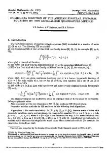
We also tested our approach for vortex states, which could be more difficult to calculate numerically due to the 1/x2 term. In figure 4 (a) we plot the vortex wave function for L = 2 and N = 100. The corresponding numerical error calculated with 100 samples over 100 units of time is plotted in figure 4 (b). Even for the vortex state L = 2, with a nonlinearity as large as N = 100 the error is very small as we can see in figure 4. 5.2. Time Evolution Problem Next we study time evolution problems with an axially symmetric trap. We take an √ initial state with N = 50 and λ = 8 which is prepared as usual at time t = 0 when we reduce suddenly the strength of the nonlinear term by a factor of 2. This corresponds to reducing the scattering length by the same factor, which can be realized in experiments [18, 19]. The system then starts to oscillate which may continue for ever as in the spherically symmetric case, albeit with different frequencies in radial and axial directions. We calculate the time evolution of the rms values of x and y: X and Y . The oscillation is more involved and in figure 5 we plot X and Y vs. t. Finally, we consider

13

Bose-Einstein condensation dynamics

again the same initial state with N = 50 at t = 0 and we double suddenly both the radial and axial harmonic oscillator trapping terms. The system starts to oscillate after the change. This is clearly exhibited by plotting X and Y vs. t in figure 6.

X, Y

4

X 2.5Y

3

2 300

305

310

t

315

320

325

Figure 5. Root mean square sizes X and Y vs. t during the oscillation of a previously formed axially symmetric condensate with N = 50 when the nonlinearity is suddenly reduced by a factor of 2.

We calculated the frequency of oscillation of rms sizes X and Y . In case of the simulation corresponding to figure 5 the principal frequency of oscillation along X direction is ν1 ≃ 0.29 and that in Y direction is ν2 ≃ 0.84. In case of simulation of figure 6 these frequencies are ν1 ≃ 0.42 and ν2 ≃ 1.16, respectively. We also considered the frequency spectrum of the time variations represented in figures 5 and 6 and we noted several frequencies, of which the principal in each case are, ν1 , ν2 , 2ν1 , 2ν2 , |ν2 ± ν1 | and q 2 (ν1 + ν22 ). Similar oscillation has been observed in a recent experiment [19] for a dynamically changing axially symmetric condensate with small nonlinearity − the observed frequencies being twice the existing harmonic oscillator trap frequencies νradial and νaxial along radial and axial directions. We repeated the simulation of figure 6 with nonlinearity zero and find that the resultant frequencies of simulation are exactly double the existing harmonic oscillator trap frequencies νradial and νaxial along radial and axial directions. In case of figure 5 these frequencies are 2νradial = 1/π ≃ 0.32 and √ √ 2νaxial = 8/π ≃ 0.90 (νaxial /νradial = 8 ≈ 2.83), which are to be compared with the frequencies ν1 ≈ 0.29 and ν2 ≈ 0.84 (ν2 /ν1 ≈ 2.90) obtained in the present simulation, respectively. The small disagreement between the two sets is due to the large nonlinearity of the present simulation. In case of figure 6 the existing trap √ frequencies are increased by 2 and hence the expected frequencies of oscillation are √ 2νradial = 2/π ≈ 0.45 and 2νaxial = 4/π ≈ 1.27, which compare well with the following results of simulation with large nonlinearity: ν1 ≈ 0.42 and ν2 ≈ 1.16, respectively (ν2 /ν1 ≈ 2.76), again the difference being due to the strong nonlinearity.

14

Bose-Einstein condensation dynamics

X, Y

4

X 2.5Y

3

2 300

305

310

t

315

320

325

Figure 6. Root mean square sizes X and Y vs. t during the oscillation of a previously formed axially symmetric condensate with N = 50 when the harmonic oscillator terms are suddenly increased by a factor of 2.

Although, we could not relate the present frequencies of numerical simulation to those of the low-energy elementary excitations of a Bose-Einstein condensate in qan axially symmetric trap [20], it is interesting to note that the nonlinear combination (ν12 + ν22 ) appears in both the cases. 6. Discussion In this paper we have presented an account of the split-step Crank-Nicholson method for the solution of the GP equation, where the nonlinear and all nonderivative terms are treated in a separate step essentially exactly via (3.5). In previous applications [4,5,7–10] of the Crank-Nicholson method to the GP equation these terms were included in the finite-difference scheme for the space derivatives. In the pioneering application of this approach Ruprecht et al [4] noted that the presence of the nonlinear potential sets a limit to the numerical stability of the method and limits the ability to find the wave function for large nonlinearity. For the spherically symmetric case, Ruprecht et al [4] produced √ results for values of nonlinearity N ≡ Na/l upto 25 2. For the axially symmetric case, the maximum of N employed by Dalfovo and Modugno [8] and by Holland and Cooper [9] were 20 and 5, respectively. Using a different method Chiofalo et al [13] produced results for values of N upto 6. However, unlike in these other methods, in the present method the results remain stable for large N , At this point we must comment on the potentially powerful split-operator method with a pseudo-spectral scheme for derivatives [21], often used in solving nonlinear Schr¨odinger-type equations. In the pseudo-spectral scheme the unknown function is expanded accurately in terms of some known polynomial (e. g. Chebyshev polynomial) over a set of grid points. As the number of terms in this expansion increases, the discrete

Bose-Einstein condensation dynamics

15

representation of the function and its derivatives becomes increasingly accurate. In the present Crank-Nicholson method the space derivative is approximated by a simple threepoint finite-difference scheme. To the best of our knowledge so far there has been no systematic application of the pseudo-spectral method to the solution of the GP equation, specially for the axially symmetric case [22]. Whether the added numerical effort in the pseudo-spectral method is compensated by the increased accuracy can only be found after a systematic comparison of the two approaches. This remains a problem of future interest. 7. Summary In this paper we propose and implement a split-step method for the numerical solution of the time-dependent nonlinear GP equation under the action of a trap with both spherical and cylindrical symmetries by time propagation starting with the initial input solution for the harmonic oscillator problem. The full Hamiltonian is split into the derivative and nonderivative parts. In this fashion the time propagation with the nonderivative parts can be treated very accurately. The spatial derivative parts are treated by the Crank-Nicholson method. In the axially symmetric case the spatial derivatives in the radial and axial directions are dealt with in two independent steps. This split-step method leads to highly stable and accurate results. The final result remains stable for millions of time iteration of the GP equation. We applied the above method for the numerical study of certain stationary and time-evolution problems with spherical and axial traps. In the spherical case stationary solutions with nonlinearity N ≡ Na/l = 5, 100, 1000, and 5000 showed accurate result with small numerical error. For a condensate with N = 2000 we studied certain timeevolution problems. We studied the resulting oscillation of the condensate when at t = 0 the trap frequency or the scattering length is altered suddenly. In all cases a clean periodic motion of the root mean square radius was noted. In the axially symmetric case the stationary solutions for L = 0 with nonlinearity N ≡ Na/l = 50 and 300 showed accurate result. A calculation of the vortex state for L = 2 with nonlinearity N = 100 showed equally precise and stable results. The numerical error was less than one percent in the central region and a couple of percents in the peripheral region. We also performed two time-evolution studies for N = 50 when the harmonic oscillator trap is doubled or the scattering length is reduced suddenly. The root mean square sizes along radial and axial directions showed clean periodic oscillation which is studied in detail. The present method seems to be very attractive for studying various dynamical evolution problems with dissipative (imaginary) interaction, which can not be handled efficiently by other methods such as variational and Thomas-Fermi methods. We have already made such an application in the study of chaotic dynamics of the Bose-Einstein condensate using the Gross-Pitaevskii equation with dissipative interaction [23].

Bose-Einstein condensation dynamics

16

Acknowledgments The work is supported in part by the Conselho Nacional de Desenvolvimento Cient´ıfico e Tecnol´ogico and Funda¸c˜ao de Amparo `a Pesquisa do Estado de S˜ao Paulo of Brazil. References [1] Ensher J R, Jin D S, Matthews M R, Wieman C E and Cornell E A 1996 Phys. Rev. Lett. 77 4984 Dadic K B, Mewes M O, Andrews M R, van Druten N J, Durfee D S, Kurn D M and Ketterle W 1995 Phys. Rev. Lett. 75 3969 Fried D G, Killian T C, Willmann L, Landhuis D, Moss S C, Kleppner D and Greytak T J 1998 Phys. Rev. Lett. 81 3811 Pereira Dos Santos F, L´eonard J, Junmin Wang, Barrelet C J, Perales F, Rasel E, Unnikrishnan C S, Leduc M and Cohen-Tannoudji C 2001 Phys. Rev. Lett. 86 3459 Bradley C C, Sackett C A, Tolett J Jand and Hulet R G 1995 Phys. Rev. Lett. 75 1687 [2] Dalfovo F, Giorgini S, Pitaevskii L P and Stringari S 1999 Rev. Mod. Phys. 71 463 [3] Edwards M and Burnett K 1995 Phys. Rev. A 51 1382 Gammal A, Frederico T and Tomio L 1999 Phys. Rev. E 60 2421 Adhikari S K 2000 Phys. Lett. A 265 91 [4] Ruprecht P A, Holland M J, Burnett K and Edwards M 1995 Phys. Rev. A 51 4704 [5] Adhikari S K 2000 Phys. Rev. E 62 2937 Adhikari S K 2001 Phys. Rev. E 63 054502 [6] Schneider B I and Feder D L 1999 Phys. Rev. A 59 2232 [7] Dalfovo F and Stringari S 1996 Phys. Rev. . A 53 2477 [8] Dalfovo F and Modugno M 2000 Phys. Rev. A 61 023605 [9] Holland M and Cooper J 1996 Phys. Rev. A 53 R1954 [10] Adhikari S K 2002 Phys. Rev. E 65 016703 Adhikari S K 2002 Phys. Rev. A 65 033616 [11] Adhikari S K 2001 Phys. Lett. A 281 265 Adhikari S K 2001 Phys. Rev. A 63 043611 Gammal A, Frederico T, Tomio L and Abdullaev F Kh 2000 Phys. Lett. A 267 305 Gammal A, Frederico T and Tomio L 2001 Phys. Rev. A 64 055602 [12] Holland M J, Jin D S, Chiofalo M L and Cooper J, 1997 Phys. Rev. Lett. 78 3801 Edwards M, Ruprecht P A, Burnett, K Dodd R J and Clark C W 1996 Phys. Rev. Lett. 77 1671 [13] Cerimele M M, Chiofalo M L, Pistella F, Succi S and Tosi M P 2000 Phys. Rev. E 62 1382 [14] Gross E P 1961 Nuovo Cimento 20 454 Pitaevskii L P 1961 Zh. Eksp. Teor. Fiz. 40 646 (Sov. Phys.-JETP 13 451) [15] Ames W F 1992 Numerical Methods for Partial Differential Equations, 3rd Ed (New York: Academic Press) [16] Dautray R and Lions J -L 1993 Mathematical Analysis and Numerical Methods for Science and Technology vol 6 (Berlin: Springer-Verlag) p 46 [17] Koonin S E and Meredith D C 1990 Computational Physics Fortran Version (Reading: AddisonWesley Pub. Co.) p 169 [18] Roberts J L, Claussen N R, Cornish S L, Donley E A, Cornell E A and Wieman C E 2001 Phys. Rev. Lett. 86, 4211 [19] Donley E A, Claussen N R, Cornish S L, Roberts J L, Cornell E A and Wieman C E 2001 Nature 412 295 ¨ [20] Ohberg P, Surkov E L, Tittonen I, Stenholm S, Wilkens M and Shlyapnikov 1997 Phys. Rev. A 56 R3346 [21] Fleck J A, Morris J R and Feit M D 1976 App. Phys. 10 129

Bose-Einstein condensation dynamics

17

Feit M D, Fleck J A and Steiger A 1982 J. Comput. Phys. 47 412 Chen J-B and Qin M-Z 2001 Electronic Transactions on Numerical Analysis (Kent State University) 12 193 Wallace R and Sloan D M 1994 Siam J. Sci. Comput. 15 776 [22] Andersson E, Calarco T, Folman R, Andersson M, Hessmo B and Schmiedmayer J 2002 Phys. Rev. Lett. 88 100401 Huepe C, M´etens S, Dewel G, Borckmans P and Brachet M E 1999 Phys. Rev. Lett. 82 1616 [23] Muruganandam P and Adhikari S K 2002 Phys. Rev. A 65 043608