arXiv:nucl-th/0101020v2 30 Apr 2001. Boundary and expansion effects on two-pion correlation functions in relativistic heavy-ion collisions. Alejandro Ayala and ...
Boundary and expansion effects on two-pion correlation functions in relativistic heavy-ion collisions Alejandro Ayala and Angel S´ anchez
arXiv:nucl-th/0101020v2 30 Apr 2001
Instituto de Ciencias Nucleares Universidad Nacional Aut´ onoma de M´exico Apartado Postal 70-543, M´exico Distrito Federal 04510, M´ exico. We examine the effects that a confining boundary together with hydrodynamical expansion play on two-pion distributions in relativistic heavy-ion collisions. We show that the effects arise from the introduction of further correlations due both to collective motion and the system’s finite size. As is well known, the former leads to a reduction in the apparent source radius with increasing average pair momentum K. However, for small K, the presence of the boundary leads to a decrease of the apparent source radius with decreasing K. These two competing effects produce a maximum for the effective source radius as a function of K. PACS numbers: 25.75.-q, 25.75.Gz, 25.75.Ld
istics of liquids is the appearance of a surface tension, such state of hadron matter could give rise to a confining boundary that acted as a reflecting surface that could affect the pion distributions just before freeze out. More recently [3], it has been proposed that the equation of state of pion matter could give rise to a phase transition from a gas phase to a more dense phase as the temperature rises close to the temperatures expected to be achieved in relativistic heavy-ion collisions, thus introducing the concept of a hot pion liquid. From a phenomenological point of view and disregarding the details of the reflection processes (which presumably depend on the energy of the incident particle), the development of a surface tension can be incorporated by imposing a sharp boundary for the pion wave functions to evolve just before freeze out. As a consequence of the finite size of the system during this stage of its evolution, the energy states form a discrete set. An important difference between statistical systems with and without a boundary is the different density of states at increasing energies, being larger in the case of the former, as illustrated in Fig. 1. The density of states of a finite system approaches that of an unbound one as the size of the system is increased. The above characteristic implies that the transverse inclusive spectrum calculated within a boundary model will exhibit a concave shape at high transverse momentum and could potentially explain the increase of the pion transverse distribution [4] in this kinematical region [5]. The increase of the pion distribution at low transverse momentum could also be explained within the same context by considering the finite chemical potential associated with the mean pion multiplicity per event [6]. More recently, it was realized that an important missing ingredient in the description of the transverse pion spectra within a boundary model was the proper inclusion of hydrodynamical expansion. The phenomenological description in terms of a bound, expanding pion system has been named the expanding pion liquid model
I. INTRODUCTION
In recent years, much experimental effort has been devoted to the production of a state of matter under the extreme conditions of high baryonic densities and/or temperatures in relativistic heavy-ion collisions. The main drive for such effort is the expectation to produce the so called quark-gluon plasma (QGP) where the fundamental QCD degrees of freedom are not confined within a single nucleon but rather over a larger volume of the order of the dimensions of a nucleus. While the properties of the QGP have been the subject of intense theoretical study and debate, much less attention has been paid to the hadronization process, or to the properties of hadronic matter at high temperatures and densities. An understanding of these is needed for a correct interpretation of the signals originating from the different stages of the collision, both for a clear distinction of a possible QGP formation but also as an interesting subject of study on its own. The most abundantly produced hadrons in relativistic heavy-ion collisions are pions. Typically, the number of pions produced one unit around central rapidity in central Au+Au collisions at energies of order 10A GeV is dNπ /dy ∼ 300 [1]. Under the assumption that the transverse dimensions of the system formed at freeze out are of order of the transverse size of an Au nucleus and that the typical pion formation time is of order 1 fm, this multiplicity implies that the average pion separation d at freeze out in the central rapidity region is of order d ∼ 0.6 fm which is less than the average range of the pion strong interaction, ds ∼ 1.4 fm. Some of the possible consequences of this large pion density produced in relativistic heavy-ion collisions where first studied by Shuryak [2] who coined the term pion liquid to refer to the situation where the pion system could not be thought of as existing as a hadron gas but rather, that its properties resembled more those of a liquid of quasipions. In particular, as one of the main character1
perform a systematic analysis of the two-pion correlation function in terms of the different parameters involved. We pay particular attention to the behavior of the effective system’s radius as a function of the average pair momentum comparing the results to what would be expected in the case of an expanding and unbound system and a pure boundary model. Finally we conclude and discuss our results in Sec. V.
and was developed in Refs. [7] and successfully applied to the description of the experimental mid-rapidity, transverse pion spectra in central Au+Au collisions at 11.6A GeV/c [1]. A further natural test ground for the model is the study of multiparticle correlations, in particular two-pion correlations.
R = 6 fm
1200
Number of States
1000
II. THE EXPANDING PION LIQUID 800
When the system of pions can be considered as confined, its wave functions satisfy a given condition a the boundary. In order to compare the results with the observed particle distributions, the shape of the assumed confining volume could play an important role. It has long been known that the particle momentum distributions are somewhat forward-backward peaked, particularly at energies of the SPS [11], even in the case of central collisions. Nevertheless, for the sake of simplicity and concreteness, here we will assume that the confining volume is spherical. Comparison of the model with data will become better in the central rapidity region where an asymmetry between longitudinal and transverse expansion is less important than in the fragmentation region. Let us emphasize that an spherically symmetric model is not essential to the basic physics discussed here and can thus be relaxed at the expense of additional computing time. This could however be necessary when comparing to data away from mid-rapidity. To incorporate the effects of an hydrodynamical flow, we notice that this ordered motion can be represented by a four-velocity field uµ = γ(r)[1, v(r)], where γ is the Lorentz-gamma factor and v(r) is the velocity vector. This field represents a redistribution of momentum in each of the fluid cells, as viewed from a given reference frame (the center of mass in this case), becoming centered around the momentum associated with the velocity of the fluid element. This behavior can be described by the substitution pµ → pµ − muµ , where m is the pion mass. The term muµ represents the collective momentum of the given pion fluid element. The eigenfunctions of the confined, expanding system of pions are thus obtained as the solutions to the equation �2 h n � ∂ i2 − i − mγ(r) + − i∇ − mγ(r)v(r) ∂t o (1) + m2 ψ(r, t) = 0
600 400 200 0
400
600
800
1000
1200
1400
E (MeV)
1600
1800
2000
2200
FIG. 1. Number of states for a spherically symmetric system with a sharp boundary at R = 6 fm (solid line) compared to a system without boundary (dotted line). Notice how the presence of the boundary makes the number of states grow faster at large energies.
A step in this direction has been taken in Ref. [8] where the effects of a pure boundary model (i.e. without collective expansion) have been introduced in the description of the two-pion correlation function. In this work, we incorporate also the effects of hydrodynamical expansion in the calculation of the two-pion correlation function. It is well known that in the study of two-particle correlation functions, the effective size of a system without a boundary decreases as the average pair momentum is increased [9] when considering the effects of hydrodynamical expansion. Physically, this effect is due to the fact that as the average pair momentum increases, the particles in the pair are more likely to be emitted from points close in space. This can also be regarded as the introduction of a further correlation in phase space for the emitted particles that effectively reduces the size of the emission region [10]. On the other hand, as emphasized in Ref. [8], for emission volumes of order of a few average pair wavelengths it is imperative to consider a full quantum density matrix in the description of particle distributions since as the average pair momentum decreases, the correlation region as a function of relative momentum increases thus effectively reducing the apparent size of the system. As we will show in this work, these two competing effects produce a maximum in the effective size of the system at a finite value of the average pair momentum. This paper is organized as follows: Section II is devoted to a recollection of the description of a bound, expanding pion system at freeze out. In Sec. III, we write the two-pion correlation function in terms of the discrete set of eigenfunctions for this kind of systems. In Sec. IV we
where we look for the stationary states subject to the boundary condition ψ(|r| = R, t) = 0 .
(2)
We consider a parametrization of the velocity vector v(r) that scales with the distance from the center of the fireball 2
v(r) = β
r ˆ r, R
statistical distribution for the ensemble is thermal. For the purposes of this section, we closely follow Ref. [8] to where we refer the reader for details. Let λ represent the set of quantum numbers {nlm′ }. The corresponding occupation number Nλ for a given state is written as
(3)
where the parameter 0 < β < 1 represents the surface fireball hydrodynamical velocity. Correspondingly, the explicit expression for γ(r) becomes 1 γ(r) = p . 1 − β 2 r2 /R2
N=
2
β r , 2 R2
(5)
d3 N d3 p 1 X = 2Eλ Nλ ψλ∗ (p)ψλ (p) . (2π)3
P1 (p) ≡
Similarly, and under the assumption of a complete factorization of the two-particle density matrix, the two pion momentum distribution can be written as
(7)
d6 N d3 p1 d3 p2 = P1 (p1 )P1 (p2 ) 2 1 X ∗ + 2E N ψ (p )ψ (p ) λ λ λ 1 λ 2 , (2π)3
P2 (p1 , p2 ) ≡
The parameters αnl and εnl are related to the energy eigenvalues Enl by
with Enl given as the solutions to � � ε2nl (l + 3/2) 2 2 − 2 , l + 3/2; αnl R = 0 . 1 F1 2 4αnl
(13)
λ
↔
α4nl = m(Enl − m)β 2 /R2 , ε2nl = Enl (Enl − 2m) ,
(11)
With the normalization adopted in Eq. (6), the one-pion momentum distribution can be written as
where 1 F1 is a confluent hypergeometric function and ′ Ylm is a spherical harmonic. The quantities Anl are the normalization constants and are found from the condition ∂ ψnlm′ (r, t) = 1 . ∂t
1 . exp(Eλ − µ)/T − 1
Let ψλ (p) represent the Fourier transformed wave function for the state with quantum numbers λ, namely Z ψλ (p) = d3 r e−ip·r ψλ (r) . (12)
2 2 Anl −iEnl t+imβr2 /(2R) m′ e Yl (ˆr)e−αnl r /2 rl ψnlm′ (r, t) = √ 2Enl � � (l + 3/2) ε2 × 1 F1 − nl2 , l + 3/2; α2nl r2 , (6) 2 4αnl
∗ d3 rψnlm ′ (r, t)
X λ
which is valid for not too large values of β. With this approximation, Eq. (1) becomes an equation for particles moving in a spherical harmonic well with rigid boundaries and can be solved analytically. The stationary states are
Z
(10)
where T is the system’s temperature and µ the chemical potential, related to the average total multiplicity N by
Since Eq. (1), with the gamma factor given by Eq. (4), can only be solved numerically, we resort to approximate the function γ by the first terms of its Taylor expansion γ(r) ≃ 1 +
1 , exp(Eλ − µ)/T − 1
Nλ =
(4)
(8)
(14)
λ
from where the two-pion correlation function C2 can be written, in terms of P1 and P2 , as (9) C2 (p1 , p2 ) =
Equation (6), along with the energy eigenvalues and definitions in Eqs. (8), (9), constitute the set of (properly normalized) eigenfunctions in terms of which the various multi-particle distributions can be expressed. The system’s finite size and the strength of the collective expansion are given in terms of the parameters R and β, respectively. In order to further proceed, it is necessary to specify the kind of ensemble that describes the statistical properties of the pion system.
P2 (p1 , p2 ) P1 (p1 )P1 (p2 ) X 2 Eλ Nλ ψλ∗ (p1 )ψλ (p2 )
= 1+ X λ
λ
2
Eλ Nλ |ψλ (p1 )|
X λ
2
Eλ Nλ |ψλ (p2 )|
.
(15) Notice that as a consequence of the factorization assumption, the correlation function is such that C2 (p, p) = 2. This is usually referred to as the completely chaotic pion production scenario [12], which is the situation expected to occur in a heavy ion collision, given the considerable rescattering experienced by pions in the production region. In contrast, if the particles were produced completely coherently, they would occupy a pure quantum
III. TWO-PION CORRELATION FUNCTION
In order to describe the situation where equilibrium has been attained (which we assume here), the proper 3
state and the two-pion momentum distribution would be simply the product of two single-pion momentum distributions, leading to the absence of the HBT effect.
IV. THE EFFECTIVE RADIUS
Armed with the eigenfunctions describing the confined and expanding pion system, Eq. (6) and with the explicit expression for the two-pion correlation function in Eq. (15), it is possible to perform an analysis to describe the behavior of C2 as a function of the several variables and parameters involved. For the spherically symmetric problem described here, the correlation function depends on the angle between the pion pair momenta. For the sake of simplicity, let us consider the case in which both momenta p1 and p2 are parallel. In this case, the summation in the numerator of the second term in Eq. (15) can be simplified, with the aid of the addition theorem for the spherical harmonics
2.5
a
K = 500 MeV
( )
C2 (q )
2
1.5
1
R = 6 fm R = 10 fm
0.5
0
0
50
100
150
200
q (MeV)
250
300
350
400
l X
2.5
b
R = 6 fm
( )
m′ =−l
2
C2 (q )
1
0
K = 300 MeV K = 500 MeV K = 700 MeV 0
50
100
150
200
q (MeV)
250
300
350
400
2.5
R = 6 fm
( ) 2
C2 (q )
1.5
1
K = 50 MeV K = 100 MeV K = 200 MeV
0.5
0
0
50
100
150
200
q (MeV)
250
300
350
′
2l + 1 . 4π
(16)
Figure 2 shows the behavior of C2 (q) as a function of q, the magnitude of the pair momentum difference q = p2 − p1 . Figure 2a shows C2 (q) for a fixed value of the magnitude K = 500 MeV of the average pair momentum K = (K2 + K1 )/2 for two values of the system radius R = 6, 10 fm. Notice that for a fixed K the width of the correlation function decreases as R is increased. Figure 2b shows C2 (q) for a fixed value of R = 6 fm and three values of K = 300, 500, 700 MeV. For the chosen values of K, the width of the correlation function increases as K is increased. Figure 2c shows C2 (q) for a fixed value of R = 6 fm and three values of K = 50, 100, 200 MeV. Notice that in this case, the width of the correlation function decreases as K is increased. In all these figures, the temperature and surface expansion velocity have been held fixed to T = 120 MeV and β = 0.5c. These values for T and β are chosen in accordance to the analysis in Ref. [13] where a correlation between the transverse flow velocity and the freeze out temperature is found in such a way that higher temperatures imply lower expansion velocities and vice versa. Since, at least for AGS energies, not too high temperatures are reached during the collision, the above value for T implies that for β, thus, the free parameters for the model can be taken either as R and T or R and β. It is also worth mentioning that in both of the above figures, the value of the chemical potential µ appearing in Eq. (15) has been fixed to µ = 0. The behavior of C2 (q) for different values of the chemical potential is shown in Fig. 3. Notice that varying the chemical potential up to values below the onset of Bose-Einstein condensation (BEC) [6] does not introduce changes in the shape of the correlation function. This can be understood by noticing that even when we increase the system’s density and thus the value of µ, we are not introducing any further correlation among the bound but otherwise non-interacting set of particles. This situation changes when, for a given temperature and system’s size, µ is beyond the value to
1.5
0.5
′
Ylm (ˆ p1 )Ylm ∗ (ˆ p2 ) =
400
FIG. 2. (a): C2 (q) for a fixed value of K = 500 MeV and for R = 6 fm (solid line) and R = 10 fm (dotted line). The width of C2 decreases as R is increased. (b): C2 (q) for a fixed value of R = 6 fm and for K = 300 MeV (solid line), K = 500 MeV (dotted line) and K = 700 MeV (thick solid line). For the chosen values of K the width of C2 increases as K is increased. (c): C2 (q) for a fixed value of R = 6 fm and for K = 50 MeV (solid line), K = 100 MeV (dotted line) and K = 200 MeV (thick solid line). For the chosen values of K the width of C2 decreases as K is increased. In all cases, the temperature, surface expansion velocity and chemical potential have been held fixed to T = 120 MeV, β = 0.5c and µ = 0 respectively.
4
numbers –and consequently with a larger spread in coordinate space– can contribute significantly to the correlation function, which in turn drops faster as a function of q with increasing K, leading to an increase in size of the apparent region of particle emission. However, for K > ηT , the collective motion dominates over the thermal component in K and the relevant physical effect that dictates the behavior of Reff is the correlation between the spatial region of emission of pions and the pair momentum introduced by the collective expansion, in such a way that faster pions are more likely to be emitted from points close in space [9] leading to a reduction in size of the apparent region of particle emission.
allow for the ground state to accommodate a significant fraction of the particle population [6]. This is also shown in Fig. 3. In this case, the ground state population has to be treated separately from the pions coming from the excited states, since the former originates from a pure quantum state, as opposed to the assumption leading to Eq. (14). The weight assigned to the pions coming from the ground state is equal to the ratio of the ground state population Ng to the total number of pions of the given species N . Correspondingly, the correlation function C2 (q) becomes flatter and the intercept with the vertical axis occurs for values smaller than 2, that is, λ = 1 − Ng /N . Thus, as the density increases, this behavior signals that for the given temperature and volume, pions are predominantly emitted from the ground state. This is in agreement with the analysis in Ref. [14].
5
R=6
fm
4 2.5 3
= 6 fm
Re�
R
2
C2 (q )
2 1.5 1
bound expanding unbound expanding bound non-expanding
1 0 0.5
Ng =N Ng =N
0
Ng =N
0
50
100
150
200
250
= 0:02 = 0:37 = 0:77
300
350
0
200
400
K
600
800
1000
(MeV)
FIG. 4. Reff for a fixed value R = 6 fm as a function of K for an expanding and bound system (solid line), an expanding and unbound system (dotted line) and a bound and non-expanding system (thick solid line). Notice that in the first case, Reff reaches a maximum at a value of K ∼ ηT , whereas for the second case, Reff decreases with increasing K and in the third case Reff grows with increasing K. Also, for the expanding and unbound system, the parameter Rgauss has been chosen in such a way as to give the same r.m.s radius than a rigid sphere with R = 6 fm.
400
q (MeV)
FIG. 3. C2 (q) for a fixed value R = 6 fm and different values of the ground state population fraction. For µ = 0 (solid line) the ground state population is negligible and λ ∼ 1. However, when the ground state population becomes a significant fraction of the total multiplicity, e.g. for µ = 315 MeV, Ng /N = 0.37 and λ ∼ 0.62 (dotted line). When almost all of the particles occupy the ground state, e.g. for µ = 317.5 MeV, Ng /N = 0.77, λ ∼ 0.23 (thick solid line) and the correlation function becomes flatter.
The behavior of Reff as a function of K is shown in Fig. 4 (solid line). Notice that the curve shows a maximum for a value of K ∼ ηT . The curve is obtained by fitting the correlation functions C2 (q) to Gaussians of the form
Another property of the bound and expanding system of pions that can be extracted from the correlation function C2 (q) is the behavior of the system’s effective radius Reff as a function of K. The relevant quantity to pay attention to is the ratio η = T /γ(R)mβ of the energy scale associated with random motion, i.e. T , to the energy scale associated with ordered motion, i.e. γ(R)mβ. For K small compared to ηT –that is, when the average pair momentum is mostly due to random motion– Reff is an increasing function of K. This can be understood by noticing [8] that increasing K corresponds to increasing both of the momenta in the pion pair. Correspondingly, the quantum states that contribute to the momentum distributions P1 and P2 are those with increasingly larger quantum numbers. But, according to Eq. (10), these states are suppressed by their statistical weight and therefore, only those other states with smaller quantum
2 g(q) = 1 + exp(−q 2 Reff ).
(17)
Equation (17) is a good description for correlation functions with large K. For small values of K, the fit is not as good. For comparison, also shown in Fig. 4 is the behavior of Reff for an expanding system without a boundary (dotted line) and for a bound system without the effects hydrodynamical expansion (thick solid line). For the former we choose a spherically symmetric phase space Gaussian distribution given by 2
2
(18) G(x, p) = e−x /2Rgauss e−γ(x)(Ep −v·p)/T , p with Ep = p2 + m2 and v and γ(x) given by Eqs. (3) 5
and (5), respectively. The correlation function is given in terms of G(x, p) by [9] R 3 d x G(x, p1 +p2 )e−i(p1 −p2 )·x 2 2 � R � . (19) C2 (p1 , p2 ) = 1+ R 3 d x G(x, p1 ) d3 x G(x, p2 )
ACKNOWLEDGMENTS
Support for this work has been received in part by CONACyT-M´exico under grants Nos. 29273-E and 32279-E.
For the bound and non-expanding system, the eigenfunctions are given in terms of Bessel functions of the first kind [6] (see also Ref. [8]). The corresponding expression for Reff is obtained from that of C2 (q) by also fitting Gaussians of the form given by Eq. (17). Notice that the curve representing the effective radius as a function of K for a bound but non-expanding system grows with K, in agreement with the analysis of Ref. [8]. In contrast, the curve representing the effective radius for an unbound but expanding system decreases monotonically as K is increased, also in agreement with the analysis of Ref. [9].
[1] E-802/866 Collaboration, L. Ahle et. al., Phys. Rev. C 57, R466 (1998). [2] E.V. Shuryak, Phys. Rev. D 42, 1764 (1990). [3] A. Kostyuk, M. Gorenstein, H. St¨ ocker and W. Greiner, hep-ph/0010076. [4] See for example: NA35 Collaboration, H. Str¨ obele et. al., Z. Phys. C 38, 89 (1988); WA80 Collaboration, R. Albrecht et. al., Z. Phys. C 47, 367 (1990); E814 Collaboration, J. Barrette et. al., Phys. Lett. B351, 93 (1995); S. Backovi´c, I. Pi´curi´c, D. Salihagi´c, D. Krpi´c and A.P. Cheplakov, Phys. Rev. C 62, 064902 (2000). [5] C.-Y. Wong, Phys. Rev. C 48, 902 (1993); M.G.-H. Mostafa and C.-Y. Wong, ibid. 51, 2135 (1995). [6] A. Ayala and A. Smerzi, Phys. Lett. B405, 20 (1997). [7] A. Ayala, J. Barreiro and L.M. Monta˜ no, Phys. Rev. C 60, 014904 (1999); A. Ayala, Rev. Mex. Fis. 45 S2, 116 (1999). [8] Q.H. Zhang and S.S. Padula, Phys. Rev. C 62, 024902 (2000). [9] S. Pratt, Phys. Rev. Lett. 53, 1219 (1984). [10] W.A. Zajc, A pedestrian’s guide to interferometry in “Particle Production in Highly Excited Matter”, pp 435, Ed. by H.H. Gutbrod and J. Rafelski, Plenum Press (New York) 1993. [11] KLM Collaboration, H. von Gersdorff et. al., Phys. Rev. C 39, 1385 (1989). [12] M. Gyulassy, S. Kauffmann and L. Wilson, Phys. Rev. C 20, 2267 (1979). [13] S. Esumi, S. Chapman, H. van Hecke and N. Xu, Phys. Rev. C 55, R2163 (1997). [14] S. Pratt, Phys. Lett. B301, 159 (1993).
V. CONCLUSIONS
In this work, we have studied the effects that a confining boundary together with hydrodynamical expansion at freeze out, play on the two-pion correlation function, in the context of relativistic heavy-ion collisions. We have argued that the confining boundary could be produced as a consequence of the high pion density that can be achieved at freeze out in central collisions. We have shown that for a given system’s volume and temperature, varying the multiplicity, and therefore the chemical potential, does not introduce any changes in the correlation function when µ is below the values for BEC. However, the intercept of the function C2 (q) occurs for values less than 2 when the chemical potential is beyond the value to allow for BEC. A similar behavior can be expected for a given pion density if the freeze out temperature is below the critical temperature for BEC. However, this is a less likely scenario in this kind of collisions. We have found the behavior of C2 (q) when varying either R or K keeping the other variable fixed. Since the importance of correlation analyses rests basically on the information that it can provide about the physical size of the system produced during the collision, a main result of the present work is the functional dependence of the effective system radius Reff with the magnitude of the average pair momentum K. We have shown that the interplay of the energy scales associated with collective and random motion, γ(R)mβ and T , respectively, produce a maximum for Reff at a value K ∼ ηT , where η = T /γ(R)mβ. The physical origins of this behavior are the combined effects of the confining boundary and hydrodynamical expansion. In the regime where K is basically due to random motion, the boundary effects are the most important and Reff grows as a function of K. However, in the regime where K is basically due to collective expansion, the effective size of the system is dictated by the correlation between the points of emission and the pair momentum and Reff decreases as a function of K. 6