1. Introduction. Dissipative Particle Dynamics (DPD) was introduced originally as .... r ?ri jr ?rij = nwall n a(Ri)1 + b(Ri)nn] (7) where Ri is the distance of the uid ...
International Journal of Modern Physics C, cfWorld Scienti c Publishing Company
BOUNDARY MODEL IN DPD M. REVENGA, I. ZU� N~ IGA, and P. ESPAN~ OL � Departamento de F��sica Fundamental, UNED, Apartado 60141 Madrid 28080, Spain
and I. PAGONABARRAGA
Instituut-AMOLF, Kruislaan, 407 1098SJ Amsterdam, The Netherlands
Received (received date) Revised (revised date) We present a model for treating the boundaries of a DPD uid. The basic idea is to model the stick boundary conditions by assuming that a layer of DPD particles is stuck on the boundary. By taking a continuum limit of this layer e�ective dissipative an stochastic forces on the uid DPD particles are obtained. The boundary model is tested by a simulation of planar Couette ow which allows to perform vicosimetric measurements. We analyze the conditions that ensure a proper stick boundary
condition for an impenetrable wall, comparing with previous methods used
1. Introduction
Dissipative Particle Dynamics (DPD) was introduced originally as an attempt to exploit the computational advantages of lattice-gas methods in computational uid dynamics and at the same time avoid the problems of being de ned in a lattice1 . The resulting algorithm was an o�-lattice algorithm in which particles evolve under mutual forces that depend on the position and velocities of the particles. These particles were interpreted as clusters of molecules that move following the hydrodynamic ow but, being still mesoscopic, they display thermal uctuations. These
uctuations were included consistently with the principles of statistical mechanics2 . The understanding and usefulness of the DPD model has grown in recent years by using the tools of kinetic theory3;4 that have shown that the model displays truly hydrodynamic behavior5 and have provided explicit expressions for the macroscopic transport coe�cients in terms of model parameters. DPD has been applied in a variety of di�erent physical problems in the context of complex uid ow1;6. It has become apparent that DPD can be understood as a version of Smoothed Particle Dynamics (SPD) that includes consistently thermal uctuations4 . SPD is a �e-mail:
pep@ sfun.uned.es 1
2 Boundary model in DPD
Lagrangian discretization of the equations of hydrodynamics in which the nodes of the moving grid can be interpreted as uid particles that interact with prescribed position and velocity dependent forces7;8. To date, however, SPD has not been suitably generalized in order to include thermal uctuations. But this is what DPD actually does. In other words, DPD can be understood as a Lagrangian discretization of the equations of uctuating hydrodynamics9;10 . As in any other method in computational uid dynamics, the issue of boundary conditions has to be addressed in DPD. Until now, only two methods have been considered in the treatment of boundary conditions in DPD. First, in order to simulate a shear ow as that generated in a Couette geometry, the Lees-Edward technique has been used11;12 , which is a way of avoiding the modelization of physical boundaries. On the other hand, when considering the boundary conditions on the surface of solid objects as in the modelization of colloidal suspensions, the method of \freezing" some portions of the uid described by DPD particles has been used1;11 . In this model, the wall boundary is not well de ned and uid particles can penetrate to some extent into the solid objects. In this paper we further exploit the idea of freezing DPD particles by presenting a generic model for treatment of the boundaries between solid objects and DPD particles. One would like to apply on the surface of the solid a no-slip boundary condition. This suggest to consider a layer of DPD particles that are stuck (or \frozen") onto the solid. By taking a continuum limit of this layer an e�ective force due to the solid onto the DPD uid particles arises. The explicit form of this force will be derived for the case of a at wall. A crucial ingredient of the model refers to the impermeability of the wall. The wall is a well de ned mathematical plane such that whenever a particle crosses the wall it is reinjected into the uid. Three di�erent models are considered: specular, Maxwellian and bounce back re ections. Very di�erent dynamical behaviour are obtained in each case, as can be observed from numerical simulations, although only the bounce-back is fully
consistent with the description of the wall as an ensemble of frozen DPD particles moving as a rigid object. As we will point out later, this is a relevant aspect regarding the modelling of the boundaries carried out in DPD so far. 2. The DPD model
The positions and velocities of the DPD particles evolve according to the following stochastic di�erential equations2;4
dri = vi dt
X
�
dvi = ? !(rij )eij eij � vij dt + 2 kBmT j 6=i
�1=2 X j 6=i
!1=2 (rij )eij dWij (1)
Here, m is the mass of the particles; is a friction coe�cient with dimensions of inverse of time; eij is a unit vector joining the pair of particles i; j ; vij = vi ?
Boundary model in DPD 3
vj ; kB is the Boltzmann constant; T is the temperature; dWij is an independent
increment of the Wienner process for each pair i; j . The function !(rij ) determines the intensity of the interaction as a function of the distance rij between particles. Following Ref.1 we select the functional form �
�
3 1? r (2) !(r) = �nr 2 rc c for 0 < r � rc and zero for r > rc . Here, rc is the range of the weight function (and, therefore, of the interaction) and n is the uid number density. The weight function is normalized in d = 2 spatial dimensions as Z
d2 r!(r) = n1
(3)
In Eqns. (1) we have neglected the conservative force present in the original algorithm in order to compare with the results of kinetic theory given in Ref.3 . Any result of a simulation must be given in non-dimensional terms. There are ve governing parameters in the model: ; rc ; kB T; �, where � is the average distance between particles, related to the number density n of particles as � = n?1=d . From these ve parameters two dimensionless parameters can be formed. Introducing the thermal velocity , vT = (kB T=m)1=2 , we select
� = �T � � dv � T r c s � �
(4)
The physical meaning of these parameters is as follows: �T = �=vT is the time taken by a particle with the thermal velocity to move an interparticle distance, whereas � = d ?1 is the time associated to the friction. More precisely, d ?1 gives the overall time scale for the decay of the velocity autocorrelation function of the DPD particles15 . Therefore, � is the ratio of these two time scales. Large � means that the particles hardly move in the time scale in which the velocity decays due to thermal uctuations. On the other hand, s is the overlapping between particles which gives the number of particles that are within the range of interaction of a given one. These two dimensionless parameters �; s x the dynamical regimes of the model. When ows in given geometries are considered, additional dimensionless parameters appear. For example, in a Couette ow between parallel in nite plates separated a distance L where the upper plate is moving at velocity V while the other one is at rest, the dimensionless parameters � = L=� and V=vT can be de ned. The parameter � is named the resolution because it gives the typical number of particles per linear dimension.
3. Flat wall model
4 Boundary model in DPD
In this section we present a model for an in nite moving at wall in contact with a DPD uid. The aim is to model stick boundary conditions for the DPD uid which means that the DPD particles which are in contact with the wall have exactly the same velocity of the wall. We will model this wall by considering that the solid wall is, in fact, made of DPD particles which are \frozen" and which interact with the uid particles in the same way as the uid particles interact with themselves. Let us analyze how a uid particle, labeled i, interact with the frozen wall particles, labeled j .
3.1. Dissipative interaction
The dissipative force that the uid particle feels as a consequence of its interaction with the wall particles is given by
FDi = ?
X j 2wall
!(rij )eij eij � (vi ? V)
(5)
where V is the velocity of any wall particle. By introducing the density eld nr = P i
�(r ? ri ), we can write this force as
FDi = ?
Z
? ri r ? ri � (v ? V) drnr !(jr ? ri j) jrr ? r j jr ? r j i
wall Z
� ? nwall
i
i
? ri r ? ri � (v ? V) dr!(jr ? ri j) jrr ? ri j jr ? ri j i wall
(6)
where we have assumed that the density eld of the wall particles is homogeneous, which will be a valid approximation if the wall particles are located at random and the number density nwall of frozen DPD particles in the wall is su�ciently large (continuum limit). The integral in (6) can be done analytically for the usually simple functional models selected for !(r). On general symmetry and geometrical grounds, it will have the following structure
M(Ri ) � nwall
Z wall
? ri r ? ri = nwall [a(R )1 + b(R )nn] (7) dr!(jr ? ri j) jrr ? i i r j jr ? r j n i
i
where Ri is the distance of the uid particle to the wall, n is the unit vector normal to the wall, and 1 is the identity matrix. The behavior of the functions a(r); b(r) is depicted in Fig. 1. If a particle is at Ri > rc then it is not in uenced by the wall. For 0 < Ri < rc the particle is subject to an anisotropic viscous force. The ratio nwall =n is the only parameter for this wall model and it governs the wall/ uid interaction.
3.2. Stochastic interaction
Boundary model in DPD 5
0.3 0.25 0.2
!; a; b 0.15 0.1 0.05 0
0
0.2
0.4
R
0.6
0.8
1
Fig. 1. The weight function !(r) (thick line) given in Eqn. (2) and the functions a(R) (thin line) and b(R) (dotted line) de ned in (7) for this weight function.
The particles on the wall also exert stochastic forces on the uid particles in such a way that in conditions of not moving boundaries, the system can reach a state of thermal equilibrium given by the Gibbs equilibrium ensemble. We could follow a similar continuum argument as for the dissipative forces but it turns out to be simpler to construct the wall stochastic force by requiring that the equilibrium distribution of the velocity of particle i is given by expf?mvi2 =2kB T g. The equation of motion of a uid particle interacting only with the wall at rest is
dvi = ? M(Ri )vi dt + FRi dt
(8)
where FRi is the stochastic aceleration. This is the equation for a Brownian particle in an inhomogeneous and anisotropic viscous medium. Therefore we expect FRi dt = �N(Ri )�dWi , where � is the noise amplitude, N(R) is a matrix and dW is a vector whose components are independent increments of the Wienner process satisfying dWi� dWj� = ��� �ij dt. Following a standard procedure13 it is possible to obtain the Fokker-Planck equation for this DPD particle with the result �
�
@t � = ? @@r � vi + @@v � ? M � vi + �2 N2 � @@v i i i
��
�
(9)
The Maxwellianpwill be a stationary solution for this equation if the detailed balance condition � = 2 kB T=m is satis ed and, in addition, N2 = M. The square root of the matrix M can be easily computed and the result is
6 Boundary model in DPD �1=2 n h i o � 1=2 (R )1 + (a(R ) + b(R ))1=2 ? a1=2 (R ) nn a N = nwall i i i i n
(10)
Boundary model in DPD 7
3.3. Impenetrable wall
If only the above forces were exerted by the walls, the DPD particles would penetrate into the region de ned as \wall" and di�use in a sort of Brownian motion. In order to avoid this undesirable e�ect, one has to introduce the particles that cross the wall back into the system . We have investigated three di�erent possibilities. The simplest one is a specular re ection at the wall which conserves momentum in the direction parallel to the wall. Note that for a DPD model with conservative forces included, the continuum limit of these forces produces an e�ective conservative force that conserves momentum in the direction parallel to the wall. We have also considered a Maxwellian re ection where the particles that cross the wall are reintroduced with normal and parallel components of the velocity extracted from Maxwellians centered at the velocity of the corresponding wall. Finally, a bounce back re ection is considered where the sign of all components of the velocity relative to the wall of the colliding particles are reversed14. Note that specular and bounce back re ections mantain the modulus of the velocity and, therefore, there are no distortions on the temperature distribution near the wall. The Maxwellian re ections enforce the correct temperature distribution. However,
as already mentioned, these three re ection mechanisms lead to di�erent
uid properties, and only bounce-back is consistent with the dissipative DPD-wall force introduced in the previous sections. However, this point has not been appreciated in the earlier modelizations of the walls in DPD. Therefore, we will analyze in more detail the implications of these di�erent re ection mechanisms in the next section.
4. Simulations We have conducted 2D simulations of a DPD uid enclosed between two parallel walls. The rst wall is located at y = 0 and at rest whereas the second wall is located at y = L and moving with velocity V . Periodic boundary conditions are used in the x direction, with a channel length of 2L. The imposed velocity gradient is V=L. We select as unit of space rc , as unit of velocity vT , and as unit of mass m. In this paper, we x the number of particles to N = 800, the resolution to � = 20 and the overlapping to s = 3 (which means an average number of neighbors of 28). The typical interparticle distance is, in this situation, � = 1=3. We will study the e�ects of varying the dynamical parameters � and the velocity gradient. The following results have been obtained with the perfectly re ecting wall. At the steady state, the velocity pro le vx (y) has been obtained by averaging the velocities of those particles that are within a layer between y and y + �y. Similar coarse grained elds have been computed for the temperature T (y) and the density n(y). For su�ciently small time steps (we use �t = 0:004) and small velocity gradients, the temperature and density elds are constant along the channel. For large time steps, some structure in the density eld appears near the wall and this is closely related to the structure that appears in the equilibrium pair distribution
8 Boundary model in DPD
function g(r) reported in Refs.3;12 , related to the fact that in an Euler al-
gorithm, detailed balance is broken at a nite time step. However, the deviations induced by the algorithm become unappreciable for su�ciently small �t. At values of V one order of magnitude larger than vT there is a noticeable increase of the temperature in the center of the channel which remains constant in time. This is due to viscous heating, which induces an increase of the
temperature in the uid. The corrections to the equilibrium temperature are quadratic in the shear rate, and teherefore these deviations are negligible at small and intermediate shear rates.
In Fig. 2 we show the velocity pro le for di�erent values of � when the imposed velocity is V = 1. We observe that linear pro les are obtained but they present slip. The amount of slip depends on � in the form depicted in Fig. 3, where it is shown the relative velocity of the uid vx (L) near the moving wall for two di�erent values of nwall =n. The larger is the ratio nwall =n, the higher is the intensity of the wall force and the better it drags the uid. 6 5
y
4 3 2 1 0
0
0.2
0.4
vx (y)=V
0.6
0.8
1
Fig. 2. Velocity pro le for di�erent values of � = 0:04; 0:08; 0:17; 0:33; 0:83; 8:33. The smaller is � the smaller is the actual gradient. Dotted lines show the range of interaction of the walls. In the central region the pro le is linear. All these pro les show slip.
We have computed the coarse grained stress eld for a xed value of an imposed velocity gradient V=L, at di�erent values of � . We have checked that the stress eld is constant along the channel, as predicted by the equations of hydrodynamics for this ow. From the stress tensor one can compute also the force exerted on the walls by the uid. This force, in turn, can be computed independently by summing all the forces that the uid particles exert on the wall. Both measurements of the force (per unit length) on the wall produce identical results.
Boundary model in DPD 9
Vslip
0.5 ++ + 0.45 3 0.4 3+ 0.35 0.3 + 3 0.25 0.2 0.15 3 + 0.1 + 0.05 3 + + 3 3 3 3 0 0 1 2 3
4
�
+ 3 5
6
7
8
+ 3
Fig. 3. Slip velocity Vslip = V ? vx (L) as a function of � . Upper curve is for nwall = 1, lower curve for nwall = 9.
If we use bounce-back re ection instead, then the measured tangential force per unit length is found to be proportional to the imposed velocity gradient. The normal force per unit length is independent of the velocity gradient and given by the ideal gas equilibrium pressure value. This Newtonian behaviour extends to high velocity gradients, so high that viscous heating becomes important and the model is, probably, not appropriate to describe a Newtonian uid. This shows that teh slip observed in Fig.2 arises due to the inconsistency between the imposed DPD-wall interaction and the specular re ection used to model a hard wall.
The ratio between the (constant) xy component of stress tensor and the velocity gradient is the shear viscosity � of the uid. For � < 1, when there is slip, two di�erent gradients must be considered, the imposed and the actual one developed by the uid which lead to two di�erent values for the shear viscosity �e� and �. The e�ective viscosity �e� is what would be measured by an experimenter in a macroscopic experiment, while � is the \actual" viscosity of the DPD uid. In Fig. 4 we plot the values of the kinematic viscosities � e� = �e� =mn and � = �=mn for an imposed velocity V = 1 for di�erent values of � (nwall =n = 9). Also shown is the theoretical prediction for the shear viscosity given by kinetic theory3. In terms of the dimensionless parameters de ned in section 2, the kinetic theory prediction for the kinematic viscosity is � � 3 s2 � � th = 21 �vT �1 + 40
(11)
10 Boundary model in DPD
14 12 10 � �vT
83
63 4
3 3
2 ++3 ++ + 3 +3 +3 +3 + 0 0 1 2 3
+ 3
+ 3 4
�
5
6
7
8
Fig. 4. Dimensionless kinematic viscosity as a function of � . Solid line is the kinetic theory prediction � th . Diamonds are for the kinematic viscosity � computed from the actual gradient and crosses are for the kinematic viscosity � e� computed from the imposed gradient. Discrepancies between � e� and � are due to slip.
We observe that � e� goes to zero in the limit of � ! 0, presents a local maximum, and when slip disappears both viscosities coincide. In turn, � follows the trend of the theoretical prediction � th with large deviations at small � . For large � the agreement between theory and simulations is fairly good. Moreover, we have observed that as the overlapping coe�cient (i.e., the number of interacting neighbors) increases, the agreement improves, a feature also observed in Ref.12 . In Ref.12 , the kinematic �k and dissipative �d contribution to the shear viscosity have been computed separately with Lees-Edwards boundary conditions. It is reported a large discrepancy between the simulation and theory prediction for the kinematic contribution �kth for high values of � (a di�erent dimensionless number is used in12 , �=rc = � ?1 s?3 where � is not to be confused with our interparticle distance), concluding that kinetic theory is not valid for large � . However, even though the ratio �k =�kth may be large, the actual value of �k is much smaller than �d in the regime of large � . The total viscosity �d + �k is, therefore, reasonably predicted by kinetic theory, even in the regime of large � .
5. Discussion
We have presented a continuum model for a at wall made of frozen DPD particles which leads to e�ective forces between the wall and DPD uid particles. The
Boundary model in DPD 11
resulting wall model has only one adjustable parameter, the wall density nwall . This parameter controls the intensity of the uid/wall interaction. When the impermeability of the wall is taken into account through specular re ections we observe that for small values of � there is slip at the boundary, which is more pronounced if the density of the wall is close to that of the uid. This a�ects the measures of the viscosity of the DPD uid in a viscosimetric experiment. This observation is of relevance when modeling colloidal suspensions by means of \frozen lumps" of uid. Note that the continuum limit of a wall made of DPD particles with conservative potential produces forces that conserve the tangential component of the momentum of the particles. For small � it is expected that slip on the surface of the colloidal particles may appear and, as a result, the torques between colloidal particles may not be well reproduced. Simulations similar to the ones presented above have been conducted also for a wall with Maxwellian re ections. In this case, the slip phenomenon still occurs, although itis less important than in the previous case (this is, the slip velocity for a Maxwellian wall with nwall = 1 as a function of � is similar to the curve for the specular re ecting wall with nwall = 9 in Fig. 3). Finally, the bounce back re ection has proven to give perfect stick boundary conditions. It is, therefore, the recommended boundary condition in order to reproduce both, impenetrability and stick boundary conditions. The continuum model presented here can be easily extended for modeling spherical solid objects. In this case, all the degrees of freedom that are used in a frozen lump model are eliminated in favor of only the position, linear velocity and angular velocity of the spheres.
Acknowledgments
Financial support from DGICYT Project No PB94-0382 and by E.C. Contract ERBCHRXCT-940546 is acknowledged. I.P. acknowledges nancial support from
FOM, and wants to thank Prof.D. Frenkel for enlightening discussions. References
1. P.J. Hoogerbrugge and J.M.V.A. Koelman, Europhys. Lett. 19, 155 (1992). J.M.V.A. Koelman and P.J. Hoogerbrugge, Europhys. Lett. 21, 369 (1993). 2. P. Espa~nol and P. Warren, Europhys. Lett. 30, 191 (1995). 3. C. Marsh, G. Backx, and M.H. Ernst, Europhys. Lett. 38, 411 (1997). C. Marsh, G. Backx, and M.H. Ernst, Phys. Rev. E 56, 1976 (1997). 4. P. Espa~nol, Europhys. Lett. 39, 605 (1997). P. Espa~nol, Phys. Rev. E 57, 2930 (1998). 5. P. Espa~nol, Phys. Rev. E 52, 1734 (1995). 6. A.G. Schlijper, P.J. Hoogerbrugge, and C.W. Manke, J. Rheol. 39, 567 (1995). P.V. Coveney and K. Novik, Phys. Rev. E 54, 5134 (1996). 7. J.J. Monaghan, Annu. Rev. Astron. Astrophys. 30, 543 (1992). 8. H. Takeda, S.M. Miyama, and M. Sekiya, Prog. Theor. Phys. 92, 939 (1994). 9. L.D. Landau and E.M. Lifshitz, Fluid Mechanics (Pergamon Press, 1959). 10. P. Espa~nol, Physica A 248, 77 (1997).
12 Boundary model in DPD
11. E.S. Boek, P.V. Coveney, H.N.W. Lekkerkerker, and P. van der Schoot, Phys. Rev. E 55, 3124 (1997). E.S. Boek, P.V. Coveney, and H.N.W. Lekkerkerker, J. Phys.: Condens. Matter 8, 9509 (1997). 12. I. Pagonabarraga, M.H.J. Hagen, and D. Frenkel, Europhys. Lett. 42, 377 (1998). 13. C.W. Gardiner, Handbook of Stochastic Methods, (Springer Verlag, Berlin, 1983). 14. A.J.C. Ladd, J. Fluid Mech. 271, 285 (1994). 15. M. Ripoll, P. Espa~nol, and M.H. Ernst, preprint.