Applied and Computational Mathematics 2014; 3(3): 90-99 Published online June 30, 2014 (http://www.sciencepublishinggroup.com/j/acm) doi: 10.11648/j.acm.20140303.14
Boundary value problems on triangular domains and MKSOR methods I. K. Youssef1, Sh. A. Meligy2 1 2
Dept. of Mathematics, Faculty of Science, Ain Shams Univeristy, Abbassia, 11566, Cairo, Egypt Dept. of Engineering Mathematics and Physics, Faculty of Engineering Shoubra, Benha Univeristy, Cairo, Egypt
Email address:
[email protected] (I. K. Youssef),
[email protected] (Sh. A. Meligy)
To cite this article: I. K. Youssef, Sh. A. Meligy. Boundary Value Problems on Triangular Domains and MKSOR Methods. Applied and Computational Mathematics. Vol. 3, No. 3, 2014, pp. 90-99. doi: 10.11648/j.acm.20140303.14
Abstract: The performance of six variants of the successive overrelaxation methods (SOR) are considered for an algebraic system arising from a finite difference treatment of an elliptic equation of Partial Differential Equations (PDEs) on a triangular region. The consistency of the finite difference representation of the system is achieved. In the finite difference method one obtains an algebraic system corresponding to the boundary value problem (BVP). The block structure of the algebraic system corresponding to four different labeling (the natural, the red- black and green (RBG), the electronic and the spiral) of the grid points is considered. Also, algebraic systems obtained from BVP with mixed derivatives are well established. Determination of the optimal relaxation parameters on the bases of the graphical representation of the spectral radius of the iteration matrices for the SOR, the Modified Successive over relaxation (MSOR) and their new variants KSOR, MKSOR, MKSOR1 and MKSOR2 are considered. Application of the treatment to two numerical examples is considered.
Keywords: SOR, KSOR, MKSOR, MKSOR1, Triangular Grid and Grid Labeling
1. Introduction The Dirichlet problem for Poisson's equation ,
,
(1)
With the unknown function u given on the boundary is considered as a model problem in the numerical treatment of elliptic boundary value problems (BVP). The structure of sparse matrices obtained from the use of the finite difference method with different labeling of the grid points had encouraged many authors to work in this area [1- 7]. The successive over-relaxation method (SOR) is an important method in solving large sparse linear systems, the vital step in using the SOR method is the determination of the optimal value of the relaxation parameter ( ), [1, 2]. The introduction of the modified successive over-relaxation method (MSOR) is due to the structure of the algebraic system obtained from the red black ordering. It is common to use square mesh for such problems, but there are domains (irregular domains) [8, 9], which would include the treatment of irregular mesh points.
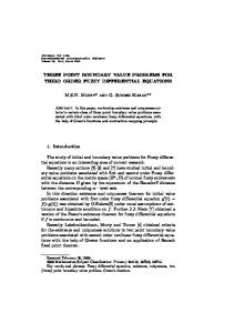
Figure 1. Equilateral triangular domain
However it is much simpler to use a mesh of the same shape as the region and avoid the use of irregular mesh points. Let us consider our domain as a unit equilateral triangle as shown in figure (1). On using the finite difference method in the triangular domain as shown in figure (1), a triangle mesh of length h=1/q is superimposed [10].
2. Poisson's Equation Let us consider the Dirichlet problem for Poisson's equation (1), defined on an equilateral triangle region of unit length. For illustration, we consider a typical grid point
Applied and Computational Mathematics 2014; 3(3): 90-99
P(x, y) as shown in figure (2) and using the finite difference method in the triangular mesh, we have:
91
with + , one is forced to represent the twofold indexed unknowns by a single indexed vector ) . This means that the internal grid points must be enumerated in some way. In the following we consider four ways of enumerating grid points and the corresponding matrix formulation () * for elliptic model problems as in the rectangular domains. -
-
3.1. Natural Order Labeling In the natural order labeling the grid points are enumerated along each row, as shown in figure (3): Figure 2. typical finite difference stencil
Assuming the function , is sufficiently differentiable and admits Taylor series expansions ,
,
√
,
2
,
2 ,
√
,
,
2
√
√
,
,
,
√
,
,
√
(2)
,
√
√
,
(3)
Figure 3. labeling the grid points in the natural order
With this labeling the coefficient matrix of the linear system () * takes the form:
And ,
√
√
,
,
√
√
,
,
√
A= (4)
For each mesh point (x,y) we replace Poisson's equation by the following difference equation: ,
3
,
√
,
,
,
√
Where
!" ! "
'$'
#$,
,
%
!"
! !
√
, &
'&'
1 -3 0 0 0 1 0 0 0 0
0 1 -3 0 0 0 1 0 0 0
0 0 1 -3 0 0 0 0 0 0
0 1 0 0 -3 0 0 1 0 0
0 0 1 0 1 -3 0 0 1 0
0 0 0 1 0 1 -3 0 0 0
0 0 0 0 0 1 0 -3 0 1
0 0 0 0 0 0 1 1 -3 0
0 0 0 0 0 0 0 0 1 -3
(8)
3.2. RBG Order Labeling (5)
Where the truncation error of the above finite difference formula approximating the equation (1) at the point (i,j) can be written as: ,
-3 0 0 0 1 0 0 0 0 0
In the red, black and green (RBG) order labeling the grid points are enumerated such that the neighboring grid points has different label (color). If we label the points with the red points first, then the black and then the green as shown in figure (4):
(6) √
(7)
Formula (6), of the truncation error guarantees the consistency of finite difference approximation with the differential equation. In the following we consider the case q=6, h=1/6, the number of internal mesh points are m=10.
3. Grid Labeling As it was in square grid in order to write the equations in the commonly used matrix formulation () * with an + , + matrix ( and m-dimensional vectors ) and *
Figure 4. labeling the grid points in the RBG order
With this labeling the coefficient matrix of the linear system () * takes the form:
92
I. K. Youssef and Sh. A. Meligy:
A=
-3 0 0 0 0 1 0 0 0 0
0 -3 0 0 1 0 0 0 0 0
0 0 -3 0 1 1 1 0 0 0
0 0 0 -3 0 0 1 0 0 0
0 0 0 0 -3 0 0 1 1 0
0 0 0 0 0 -3 0 1 0 1
0 0 0 0 0 0 -3 0 1 1
1 0 1 0 0 0 0 -3 0 0
0 1 1 0 0 0 0 0 -3 0
Boundary Value Problems on Triangular Domains and MKSOR Methods
0 0 1 1 0 0 0 0 0 -3
(9)
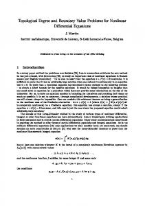
Figure 6. labeling the grid points in the spiral order
3.3. The Electronic Order Labeling In the electronic order labeling the grid points are
With this labeling the coefficient matrix of the linear system () * take the form: -3 0 0 0 0 0 0 0 1 0
enumerated as shown in figure (5):
A=
Figure 5. labeling the grid points in the electronic order
With this labeling the coefficient matrix of the linear system () * takes the form
A=
-3 0 1 0 0 0 0 0 0 0
1 -3 0 0 1 0 0 0 0 0
0 1 -3 0 0 1 0 0 0 0
0 1 0 -3 0 0 0 1 0 0
0 0 1 1 -3 0 0 0 1 0
0 0 0 0 1 -3 0 0 0 1
0 0 0 1 0 0 -3 0 0 0
0 0 0 0 1 0 1 -3 0 0
0 0 0 0 0 1 0 1 -3 0
0 0 0 0 0 0 0 0 1 -3
(10)
The coefficient matrix in (10) appears like that in (8) of the natural ordering but the order of the diagonal blocks is reversed. 3.4. The Spiral Order Labeling In the spiral order labeling the grid points are enumerated such that all the grid points on a peripheral circuit are grouped together as shown in figure (6):
1 -3 0 0 0 0 0 0 0 1
0 1 -3 0 1 0 0 0 0 0
0 0 1 -3 0 0 0 0 0 0
0 0 0 1 -3 0 0 0 0 1
0 0 0 0 1 -3 0 1 0 0
0 0 0 0 0 1 -3 0 0 0
0 0 0 0 0 0 1 -3 0 1
0 1 0 0 0 0 0 1 -3 0
0 0 1 0 0 1 0 0 1 -3
(11)
4. Elliptic Equations with Mixed Derivatives Partial differential equations with mixed derivative terms appear in many applications [7, 8, 9]. The treatment of mixed derivative terms introduces many problems especially on irregular domains [9]. Triangular grids give accurate representation for many domains. In the following we consider a simple elliptic equation defined on a triangular domain and introduce the structure of the linear algebraic system corresponding to the four grid labeling considered in the model problem of Poisson's equation. We introduce a formal parameter r to illustrate the correspondence of the coefficient matrices in the existence of mixed derivative term with the case without this term. 4.1. Simple Elliptic Equation with Mixed Derivative Term We introduce the main ideas trough a simple elliptic partial differential equation of the form ,
(12)
Using the difference representations in (2), (3) and (4) equation (12) can be approximated by the following difference equation: √
,
√
1
√
,
√
,
√
√
,
,
1
√
√
3
,
,
(13)
Where the truncation error at any point (i,j) can be
Applied and Computational Mathematics 2014; 3(3): 90-99
written as: !"
,
! "
#$,
!"
%
! !
, &
(14)
'$' , '&' Where Using the same notations described in section (2), the structure of the coefficient matrices corresponding to the four labeling can be obtained as follows: √
√
4.1.1. Natural Order Labeling
A=
-3 1 0 0 0 -3 1 0 0 0 -3 1 0 0 0 -3 1+r - r 0 0 0 1+r - r 0 0 0 1+r - r 0 0 0 0 0 0 0 0 0 0 0 0
r 1-r 0 0 -3 0 0 1+r 0 0
0 r 1-r 0 1 -3 0 -r 1+r 0
0 0 0 0 0 0 0 0 r 0 0 0 1-r 0 0 0 0 r 0 0 1 1-r r 0 -3 0 1-r 0 0 -3 1 r - r 0 -3 1-r 0 1+r - r -3
Where / , We note that if we put formally / obtain the matrix in (8) √
A=
0 -3 0 0 1 0 0 0 -r 0
0 0 -3 0 1-r 1 1+r r 0 -r
0 0 0 0 0 -r -3 0 0 -3 0 0 1-r 0 0 1 0 1+r r 0
r 0 0 0 0 -3 0 1-r 0 1+r
0 1 0 0 0 1-r r 1+r 1 -r 0 0 0 0 r 0 -r 0 -3 0 - r 0 -3 0 1-r 0 -3 1 0 0
We note that if we put formally /
matrix in (9)
0 0 1-r 1+r 0 r 0 0 0 -3
0 we
A=
We note that if we put formally / matrix in (10) 4.1.4. The Spiral Order Labeling
0 0 r 0 0 0 1-r r 0 0 0 1-r 0 0 0 0 0 0 0 0 1-r 0 0 1+r -3 1+r 0 0 r -3 1+r - r 0 r -3 1 0 1-r 0 -3
(18)
0 in (18), we obtain
Corresponding to each labeling there is a linear system of m linear equations in m unknown function values; m is the 1 1 10), so it can number of internal grid points (+ be written as a matrix equation () * It is clear that the system has unique solution; the matrix of coefficients is diagonally dominant. Also, for large values of 2 or accordingly + the system is sparse [2]. The iterative methods for solving linear systems of algebraic equations: We consider a linear system of m equations in the following form: ∑89 4
(16)
0 we obtain the
0 0 0 0 0 0 0 0 0 0 0 0 1 r 0 0 0 1 r 0 0 0 1 r -3 1-r 0 0 - r -3 1-r 0 0 - r -3 1-r 0 0 - r -3
0 0 0 0 1-r -3 -r 1 0 r
5. Iterative Methods (15)
4.1.3. The Electronic Order Labeling -3 1 r 0 0 0 0 -3 1-r 1 r 0 1+r - r -3 0 1 r 0 0 0 -3 1-r 0 0 1+r 0 - r -3 1-r 0 0 1+r 0 - r -3 0 0 0 0 0 0 0 0 0 1+r 0 0 0 0 0 0 1+r 0 0 0 0 0 0 1+r
0 0 r 1-r -3 -r 0 0 0 1
We note that if we put formally / the matrix in (11)
4.1.2. RBG Order Labeling -3 0 0 0 0 1+r 0 0 0 0
A=
-3 1 0 0 0 -3 1 0 0 0 -3 1 0 0 0 -3 0 0 1+r - r 0 0 0 0 0 0 0 0 0 0 0 0 1+r - r 0 0 0 1+r - r 0
93
*; 6
1, 2, 7 , +
(19)
The system (19) can be written in the matrix form as: (
*
(20)
Where (, is the coefficient matrix, * is a known column of constants matrix and is the unknown. We express the matrix ( as: (
:
;
)
(21)
With : is a diagonal matrix with the same diagonal elements in (, and ;, ) are the strictly lower and upper triangular parts of (, respectively [2].
5.1. Successive Over-Relaxation Method (SOR)
The point SOR method for the system (19) can be written (17)
0 we obtain the
1
?@@
∑
*
< 9
4