´ tica: Teor´ıa y Aplicaciones 2004 11(1) : 17–40 Revista de Matema cimpa – ucr – ccss
issn: 1409-2433
bounded variables nonlinear multiple criteria optimization using scatter search Ricardo P. Beausoleil∗ Recibido/Received: 14 May 2002
Abstract This paper introduces an adaptation of multiple criteria scatter search to deal with nonlinear continuous vector optimization problems on bounded variables, applying Tabu Search approach as diversification generator method. Frequency memory and another escape mechanism are used to diversify the search. A relation Pareto is apply in order to designate a subset of the best generated solutions to be reference solutions. A choice function called Kramer Selection is used to divide the reference solution in two subsets. The Euclidean distance is used as a measure of dissimilarity in order to find diverse solutions to complement the subsets of high quality current Pareto solutions to be combined. Convex combination is used as a combined method. The performance of this approach is evaluated on several test problems taken from the literature.
Keywords: Tabu Search, Scatter Search, Nonlinear Optimization. Resumen El art´ıculo presenta una adaptaci´ on del algoritmo de B´ usqueda Dispersa Multiobjetivo para la solucionar problemas de optimizaci´ on vectorial no lineales continuos, empleando un enfoque de B´ usqueda Tab´ u como un m´etodo generador de soluciones diversas. Memoria de Frequencias y otros mecanismos de escapes son utilizados para diversificar la b´ usqueda. La relaci´ on Pareto es aplicada para designar un subconjunto de las mejores soluciones generadas a ser soluciones de referencias. Una funci´ on de selecci´ on denominada selecci´ on de Kramer se utiliza para dividir al conjunto de referencia en dos subconjuntos. La distancia Euclideana es usada como una medida de disimilaridad a modo de hallar soluciones diversas que complementen los subconjuntos de soluciones potencialmente Pareto de alta calidad a ser combinadas. Como m´etodo de conbinaci´ on usamos la combinaci´ on convexa. El desempe˜ no de este enfoque es evaluado con diferentes problemas de pruebas tomados de la literatura. ∗
Centro de Matem´ atica y F´ısica Te´ orica, Calle E # 309 esq. a 15, Vedado, Ciudad de La Habana, C.P. 10400, Cuba. Fax: +(537) 33 33 73. E-Mail:
[email protected]
17
18
R. Beausoleil
Palabras clave: B´ usqueda Tab´ u, B´ usqueda Dispersa, Optimizaci´on No Lineal. Mathematics Subject Classification: 90C29, 90B50.
1
Introduction
This paper presents one way to apply Tabu Search and Scatter Search in nonlinear multiobjective optimization, using a search followed by multiple criteria decision making approach, that is, generating a set of non-inferior solutions and then select one or more of these on the basis of multiple criteria decision making. Following our methodology [3], we use a Pareto-Based Approach, that uses a Choice Function to rank solutions. An adaptation of tabu search for nonlinear optimization to a multiobjective environment is used to generate an initial set of diverse non-inferior solution. Also this adaptation is extended to incorporate a scatter search approach to improve these solutions toward the Pareto frontier. To apply our strategy, we consider two approaches: (1) directional search, where a transition from one point to another occurs by reference to feasible directions; (2) scatter search, where successive collections of points are generated from weighted combinations of reference points. The organization of the paper is as follows. Notation and general methods are treated in section 2. Section 3 presents a nonlinear multiobjective tabu search approach. Section 4 is devoted to scatter search applied to nonlinear optimization. Section 5 gives some test problems for nonlinear multiobjective problems. Section 6 contains conclusions.
2
Notation and general methods
Formally, we can state a quantitative decision making as follows. Decisions have a quantitative character, a decision(or solution) x ∈ Ex , where Ex denotes a decision space, and X ⊆ Ex is a set of admissible decisions. We have functions f1 , f2 , . . . , fr , defined over a set of situations X × V , where V is a finite set of uncertain factors values. Then for each situation (x, v), where x ∈ X and v ∈ V , we have a vector function F (x, v) = (f1 (x, v), f2 (x, v), . . . , fr (x, v)). For deterministic problems the vector function F (x) determines the quality of the decision x.
2.1
Non-dominance
We will refer to an objective function vector as a point. The point F (x) dominates the point F (x0 ) if and only if F (x) ≥ F (x0 ) and F (x) 6= F (x0 ) (i.e. if ∀i : fi (x) ≥ fi (x0 ) and fi (x) > fi (x0 ) for at least one objective i). The point F (x) is dominated by the point F (x0 ), if the point F (x0 ) dominates the point F (x). If a point is not dominated by another point, it is called a non-dominated point. Solution x is superior to solution x0 if the point F (x) dominates the point F (x0 ).
bounded variables nonlinear multiple criteria optimization
19
Solution x is inferior to solution x0 if the point F (x0 ) dominates the point F (x). If the point F (x) is non-dominated, then x is non-inferior. The set of all non-inferior solutions is sometimes refereed to as the Pareto Optimal Set. The set of all non-dominated points in the objective space is refereed to as the Pareto Frontier.
2.2
Choice function
In order to obtain a reference set of solutions that encourages the search toward the Pareto frontier, an optimality principle is used: “Selection by a number of dominant criteria” [19]. For all x, x0 ∈ X, let q(x, x0 ) be the number of criteria for which the decision variable 0 x improves the decision variable x, then QX = maxx0 ∈X q(x, x0 ), x ∈ X can be see as a discordance index if x is assumed to be preferred to x0 . Then the Kramer Choice function is defined as follows: C K (X) = {x0 ∈ X|QX (x0 ) = minx∈X QX (x)}.
3
Nonlinear multiobjective tabu search
Tabu Search TS is a strategy based on the use of prohibition-based techniques and “intelligent” schemes as a complement of basic heuristic algorithms like local search, with the purpose of guiding the basic heuristic beyond local optimality. In a nonlinear optimization context, a standard move is m(x) = x + hd, where d is a specified direction vector, such as a generalized gradient, and h is a scalar step size. In our approach we use a similar strategy. By the standard TS approach, a move is classified tabu and excluded from consideration if it reverses a recent previous move. An adaptation of Tabu search strategies for preventing move reversals in nonlinear context is applied, see [11]. A sequential fan strategy is used to create our neighborhood. Also, a TS strategy to guide the search toward the Pareto frontier is introduced. A weighted sum approach is used as a decision rule to transit from one solution to another. Recency and frequency based memory for diversification are used in our approach.
3.1 3.1.1
Directional search strategy Neighborhood (move description)
In the following we suppress reference to the indexes of the different variables for noL tational convenience, and use the following move: m(x) = x ht d where we have ht as the step sizes at iteration t, ht positive. Let ∆xt = ht d, and assume the condition [x − ∆xt , x + ∆xt ] ∩ [a, b] 6= ∅ holds. Then, ∆xt ≤ |x − a| if the operation in the move is “-”, in this case d = |x − a|, and ∆xt ≤ |b − x| if the operation in the move is “+”, then d take the value |b − x|, in both cases, x ranges over [a, b], ht ∈ A = {r/fan : r is a random number in a set {2, 3, . . . , fan}}, where fan is the number of trial solutions created, as explained above. In our implementation we propose to move as maximum four variables, in the case of more than four variables we can use random controlled and frequency memory to select the move-variables.
20 3.1.2
R. Beausoleil
Status tabu
We focus our attention on tabu conditions based on move reversals. For our purpose, we will select variables as a basis for defining move attributes, identifying the change values in going from one solution to another [11]. Tabu restrictions are imposed to prevent moves that bring the values of variables “too close” to values they held previously. Specifically a move is tabu if it creates a solution x which lies closer than a specified tabu distance dist to any solution visited during the preceding t iterations. The implementation of this rule is as follows: the variable x0 is excluded from falling inside the line interval bounded by x − w(x0 − x) and x + w(x0 − x), where 1 ≥ w > 0, when a move from x to x0 is executed. In our approach we use a tenure = 7 for the tabu memory structure and one tabu list for each variable. 3.1.3
Memory structures
We briefly illustrate the meaning of the variables and memory structures used. An elementary move is indexed by the variable ht , the step size. The tabu distances are saved in records that contain the lower and the upper bounds of these distances, tabu[current].lower and tabu[current].upper, where current is a pointer to tabu list, tabu[current].IX and tabu[current].IY stores the “from” and “to” variables, we have a similar tabu list for each variable. Our tabu lists are a circular one. Our approach uses a frequency-based memory denoted by residence, this is a record that has two entries, residence[j].range contains the upper bound of a sub-range of [a, b], and residence[j].freq contains the number of times that the associated sub-ranges have been visited, j is an index. A similar record is associated to each variable. 3.1.4
Candidate list strategy
We use a simplified version of a sequential fan strategy as candidate list strategy. The sequential fan generates p best alternative moves at a given step, and then to create a fan of solution streams, one for each alternative. The best available moves for each stream are again examined, and only the p best moves overall provide the p new streams at the next step. In our case, taking p = 1, we have in each step for ht ∈ A one stream and several points equal to fan. 3.1.5
Search by goals
Our implementation uses as move attribute, variables that change their values as result of the move. We represent change represented by a difference of values fi (x0 ) − zi∗ ∀i = 1..r , x0 ∈ X where x0 was generated from x by a recent move, x is a current solution and Z ∗ is a reference solution, Z ∗ = (z1∗ , . . . , zr∗ ). A thresholding aspiration is used to obtain an initial set of solutions as follows: without lost generality, assume that every criteria is maximized. Notationally, let ∆f (x0 ) = (∆f1 (x0 ), . . . , ∆fr (x0 )) where ∆fi (x0 ) = fi (x0 ) − zi∗ , i ∈ {1, . . . , r}.
bounded variables nonlinear multiple criteria optimization
Let
21
if ∆fi (x0 ) > 0, preference indifference if ∆fi (x0 ) = 0, ∆fi (x0 ) = nonpreference if ∆fi (x0 ) < 0,
A goal is satisfied, allowing x0 to be accepted and introduced in S if (∃∆fi (x0 ) = preference) or (∀i ∈ {1, . . . , r}[∆fi (x0 ) = indifference]), otherwise it is rejected. The point Z ∗ is updated by zi∗ = max fi (x0 ), ∀i ∈ {1, . . . , r}, x0 ∈ S. 3.1.6
Weighted sum approach
In order to measure the quality of the solution we propose to use in our tabu search approach an Additive Function Value AF V with weighting coefficients λi (λi ≥ 0), representing the relative importance of the objectives. We want to set the weights (λi , i = 1, . . . , r) so that the solution selected is closest to the new aspiration threshold. Therefore each component in the weight vector is set according to the objective function values. We would give more importance to those objective that have greater differences between the quality of the trial solution and the quality of the reference solution. The influence is given by an exponential function exp(−si ), where si is obtained as follow si =
|fi (x0 )−zi∗ | |zi∗ |
λi = 2 − exp(−si ) X AF V (x0 ) = λi ∆fi (x0 ) i=1,r
Note that in the cases of greater differences the value of the AF V is less modified that in the cases of lesser differences, making that the chosen solution is close to the new aspiration threshold. 3.1.7
Frequency-based memory and diversification strategy
Our diversification method employs a frequency memory to encourage the search to unvisited regions or less visited regions. We accomplish this by dividing the range of variables b − a into sub-ranges of equal size as in [14]. The threshold T determines the number of times that one sub-range can be visited without penalizing. A diversifying movement is executed when residence.freq[j] is greater than T . We modify the value of AF V (x0 ) as follows: AF V (x0 ) = AF V (x0 ) − freq × AF V (x0 ), where freq is an addition of the freqtotal entries of type residence.freq associatedP to the variables and subranges that hold the condition f req(x0 ) > T , and freqtotal = i f reqi , we would have for each variable a Psubranges threshold T . T is equal to max{Round( i=1 f reqi /subranges), 1}, where Round is the closest integer. The frequency memory is maintained over all iterations and in the two phases of this algorithm.
22 3.1.8
R. Beausoleil
Pseudo code for our TS approach
Skeleton of our Tabu Procedure Taboo { (Initialization step) Set a and b equal to the lower and upper bounds respectively of the variables Generate a feasible solution x (the midpoint of each interval) z ∗ = F (x) (Setting the reference point) S=x for i = 1 to numiter newelement = FALSE UpdateThreshold x0 =Candidate(x) Make tabudist(x, x0 ) x = x0 z ∗ = nextz ∗ endfor } Procedure Make tabudist(x, y) { (Record the lower and the upper bound of the interval where the variable is excluded) tabu[current].lower=x − w(y − x) tabu[current].upper=x + w(y − x) tabu[current].IX=x tabu[current].IY=y (update the current point of tabu list) if current = tenure then current = 1 else current = current+1 } Procedure Update Criterion 0 { if AF V (bestx0 ) < AF V (x ) ) then AF V (bestx0 ) = AF V (x0 ) bestx0 = x0 } Procedure Candidate(x) { tabuflag=TRUE AF V (bestx0 ) = −∞ num tabu=0 repetition=0 while tabuflag tabuflag = FALSE for i = 1 to fan x0 =Move(x) if not Is tabu(x0 ) or Aspiration(x0) then
bounded variables nonlinear multiple criteria optimization
23
if Aspiration(x0) then Update Criterion else if D(x0 ) 6= ∅ and E(x0 ) = 0 then Update Criterion else num tabu=num tabu+1 endfor if num tabu = fan then tabuflag=TRUE Reduction tabu distance x0 = Candidate(x) endwhile } We denote E as the set of efficient moves and D the set of deficient moves, where a deficient move is a move that not satisfies the aspiration level, in otherwise the move is efficient. Then, we define the best move as [m ∈ E(x0 ) : c(x0 ) = max{c(x0 ), x0 = m(x)}] if E(x0 ) 6= ∅, in the case where E(x0 ) = ∅ and D(x0 ) 6= ∅ then, select [m ∈ D(x0 ) : c(x0 ) = max{c(x0 ), x0 = m(x)}]. In the above algorithm we have the following escape mechanism: when the forbidden moves grow so much that all movements become tabu and none satisfies the aspiration level, a reduction mechanism is activated and the tabu distance in each list is reduced, then the number of forbidden moves is reduced. Function Variation(x) (x−a) { UB=min{ b−x) d , d } 2U B h= s variation=h ∗ d } Function Move(x) { Step size move = x+Variation } Function Is tabu(x) {(return the boolean value TRUE if, after the movement, the value x fall inside one interval bounded by the value lower and upper contained in the tabu list. The boolean value is FALSE otherwise) Is tabu = FALSE if iter ≤ list size then point = 1 else point = current+1 while point 6= current (x can be a portion of the decision variable) if tabu[point].lower < x < tabu[point].upper then Is tabu=TRUE break if point = list size then
24
R. Beausoleil
point = 1 else point = point+1 endwhile } Procedure Aspiration(x) (Return the boolean value TRUE if the function values, after the movement, permit to be accepted the point as probably non-dominated point) newelement = FALSE for i = 1 to r delta[i] = f0 [xi ] − zi∗ if (∃ delta[i] = preference i ∈ {1, . . . , r}) or (∀i ∈ {1, . . . , r} [delta[i] = indifference]) then X = X + x0 Obj = F (X) newelement = TRUE Update freq(x) if freq(x0 ) − T > 0 then AF V (x0 ) = Penalize(AF V (x0 )) next z ∗ = max{fi (x0 )}; x0 ∈ X endif endif } Procedure Reduction tabu distance(x) {(Change the bounds in the tabu list) w=w/2 for all i belonging to tabu list tabu[i].lower=tabu[i].IX - w(tabu[i].IY-tabu[i].IX) tabu[i].upper=tabu[i].IX + w(tabu[i].IY-tabu[i].IX) }
4
Multiobjective scatter search “MOSS”
4.1
Overall view
Scatter Search operates on a set of solutions, the reference set, by combining these solutions to create new ones. In our approach the mechanism for combining solutions is such that a new solution is created from a linear combination of two other solutions. We define the following sets: X: a set of trial points, from which all others sets derive. R: a set of current reference solutions, constituted by non-dominated elements of S. R1: a set of high-quality non-inferior solutions, composing a subset of R. R2: a difference set between R and R1.
bounded variables nonlinear multiple criteria optimization
25
T : a set of tabu solutions, composing a subset of R excluded from consideration to be combined as first solution in a convex combination. T 1: a set of tabu solutions, composing a subset of R excluded from consideration to be combined during t generation as second and third elements in the subset combined. P : a pareto set, constituted of non-inferior solutions of S. The reference set is constructed with the union of R1 and R2, where R1 = C k and R2 = P \ C k . Scatter Search has three main loops: 1) a “for loop” that controls the maximum number of iterations, 2) a “while loop” that monitors the presence of new elements in the reference set and 3) a “for loop” that controls the examination of all subsets that hold the tabu restriction imposed. As a basis for creating combined solutions we generate subsets x0 and for each x0 use a solution combined method, generating solution in a line. We use weights to sample points from the line. Avoiding the duplicated strategies already generated can be a significant factor in producing an effective overall procedure. The control is limited to these solutions that hold the condition of being Pareto. Our algorithm is provided by “critical event design” that monitors the current solutions in R and in the combined set Ω(x0 ). The elements considered in the critical events design are the values of the objectives, and the decision variables of the current Pareto solutions generated. The new solutions are put in the set Ω(x0 ) if they do not belong to the set of critical events. If all subsets have been examined then, the algorithm subtracts the non-dominated solutions ΩP ⊆ ∪Ω(x0 ) \ C, where C is a critical event set. New elements are incorporated into R if |P ∩ R| < |P | where, P ⊆ ΩP ∪ R.
4.2
Choosing subset of reference points
Our approach is organized to generate two different collections of subsets of R, which we refer to as subset1 and subset2, see [12]. The type of subsets we consider are as follow: subset1: 3-elements subsets of R1 where the second and third elements are the most dissimile to the first. subset2: 3-elements subsets derived from the two first elements of a subset1 by augmenting it to include the most diverse solution relative to it from R2.
4.3
Memory structures
Let S size denote the current number of solutions in the trial point set. S size begins at 0 in an initialization step and is increased each time a new solution is added to the trial points set, until reaching the value (max size - cardR) or all subsets of reference points were examined. At each step, S stores the current trial solution inX[trial[i]].x, the values of the objective functions are recorded in X[trial[i]].F where F contains several fields (f1 , . . . , fr ).
26
R. Beausoleil
X[trial[i]].T is a boolean variable identifying that the solution was combined in a previous iterations as first element in the subset combined. X[trial[i]].T2 records the time that this solution will be forbidden as second and third solution in a subset combined . A solution x is not permitted to be recorded if it duplicates another solution already in R. We speed the check to see if one solution duplicates another by keeping information about the objective functions and the decision variables. If one solution is duplicated, it is eliminated. Several associated location are defined: pareto[i], i = 1 to psize, indicates the position in S of non-inferior current solutions, that is, X[pareto[i]] is a current pareto solution, kramer[i], indicates the best non-inferior solutions, refset1[i] i = 1 to cardR1, the high quality current Pareto solutions and refset2[i] i = 1 to cardR2, that take a role as a diverse subset of current non-inferior solutions.
4.4
Pseudo code scatter search
Procedure Scatter { Set R = ∅ Set C = ∅ generation=0 For 1 to MaxIter (Generate an initial reference set of trial points) Taboo (SS Phase) P =ParetoSet(S) if | P |> 1 then R1 = KramerChoice(P ) R2 = P \ KramerChoice(P ) R = R1 ∪ R2 iter=0; (In our implementation we take MaxGeneration = 2) while(0 < MaxGeneration)or(ratio ≥ β) Calculate the number of MaxSubset that includes at least one new element For counter = 1 to MaxSubset Generate the new subset x0 from R with a number of elements ranging from 2 to 3(optional) Apply line search approach to obtain a set Ω(x0 ) of new solutions EndForMaxsubset Obtain ΩP ⊆ Ω(x0 ) \ C (ΩP is the current Pareto set) If |P | = 1 then Break ratio =| P ∩ R | / | P | R1 = KramerChoice(P )
bounded variables nonlinear multiple criteria optimization
R2 = P \ KramerChoice(P ) R = R1 ∪ R2 generation = generation + 1 MaxGeneration = MaxGeneration − 1 endwhile endif endMaxiter } Procedure Sigma { for i = 1 to S size P X[trial[p]].sum= j=1..r X[trial[p]].f[j] } Procedure Is Pareto { if ∃i = 1..psize, j = 1..r : X[trial[p]].f[j] < X[pareto[i]].f[j] then Is Pareto=true else Is Pareto=false } Procedure Critical Condition { if X[trial[p]].F=X[pareto[i]].F then Critical Condition=true else Critical Condition=false } Procedure Is Critical { Is Critical=false for i=1 to psize if X[pareto[i]].sum=X[trial[i]].sum if Critical Condition then Is Critical=true break } Procedure Non Dominated { for p=2 to S size if not Is critical(trial[p] and Is Pareto(trial[p]) then psize=psize+1 pareto[psize]=trial[p] } Procedure Pareto { Sigma Sort X[pareto[1]].F=X[trial[1]].F psize=1 Non dominated } Procedure KramerChoice {(Records the index of the selected solution
27
28
R. Beausoleil
array and the cardinal of the choice set in size) Q=r+1 i=1 while (i ≤cardR) QI[i]=0 j=1 while (j ≤cardR) d=Discordance(R[i].F(x),R[j].F(x)) QI[i]=max(d,QI[i]) j =j +1 ifQI[i]< Q then Q = QI size=1 selection[size]=i else size = size+1 selection[size]=i endwhile endwhile KramerChoice=selection } Combining Strategy Let Ω(X) = x + $(x0 − x), f or $ = 1/2, 1/3, 2/3, −1/3, −2/3, 4/3, 5/3, and x, x0 ∈ x0 The most dissimile solution relative to x0 is measured with the max-min criterion, that is, maximize the minimum value of a dissimilarity measure. We take as dissimilarity measure the Euclidean measure. The strategy to create the Ω set is as follows: Let x be the first element choice, x0 the second and x00 the third, the selection of each elements is makes with the max-min criterion then, we apply the following rules: 1. Generate new trial points on lines between x and x0 . 2. Generate new trial points on lines between x00 and x. 3. Generate new trial points on lines between x00 and x0 . 4. Generate one solution by applying x0 +
x−x0 2 .
5. Generate one solution by applying x00 +
x−x00 2 .
6. Generate one solution by applying x00 +
x0 −x00 2 .
In the cases 4, 5, and 6 generate new trial points on lines that join each reference point with one of the trial points generated using convex combination methods. In this case the search relies searches star from middle trial points. If we have only two points initially then, the third point is obtained by linear combination of this two points.
bounded variables nonlinear multiple criteria optimization
29
In the special case where C k = 1 then, the approach begins by selecting the first element pertaining to R1, denoting it by x, the second element is selected from R2, denoting it by x0 , if the cardinal of R2 is greater than 1 then, the third element is selected from R2 to maximize its distance from the first and second elements, denoting it by x00 , in other case the third element is created by a linear combination of the two elements selected above, and then to apply the above scheme of combination explained. Procedure Combine { (Create subset type 1 and 2, and combine) for i = 1 to cardR1 if not R[refset1[i]].T then Let R[refset1[p]].x = x ∈ x0 Let the most dissimile R[refset1[p]].x the second element in x0 Set R[refset1[p]].T1=generation+tenure Put the most dissimile R[refset1[p]].x relative to x0 the third element z Create Ω(x0 + z) Set R[refset1[p]].T1=generation+tenure Set R[refset1[i]].T=TRUE if cardR2 6= 0 then Combine2 endfor } Procedure Combine2 { (Create subset type 2) Put the most dissimile R[refset2[p]].x relative to x0 ∈ x0 Create Ω(x0 ) Set R[refset2[p]].T1=generation+tenure }
4.5
Restarting solutions
In order to build a new set S in the next iteration, we generate a new seed point using the history of the search looking for the subranges unless visited taking the middle points of these subranges as components of the new seed point, and then use the diversification generator. Initialise the generation process with the solutions currently in R.
5
Computational experiments
In this section we will examine the performance of our algorithm on several test problems with one, two and three variables since these may be plotted.
5.1 5.1.1
2-objectives test problems Problem 1 Schaffer’s F2
First we examine the algorithm convergence properties and the diversity of the solutions in the frontier using Schaffer’s F2 function [21]. f1 (x) = x2 and f2 (x) = (x − 2)2
30
R. Beausoleil
This is a simple function with a single decision variable and two objectives to be minimized. The Pareto front is where the tradeoff exits between the two functions. That is, for 0 ≤ x ≤ 2.00, one of the functions is decreasing while the other is increasing. The problem was solved on the domain −100 ≤ x ≤ 100. Figure 1(a) shows the first approximation to the Pareto set in the first generation obtained from tabu search, figure 1(b) shows that the points were well distributed over all Pareto frontier in this generation. F2 is an easy problem for our MOSS, the initial reference solutions contains several solutions on the frontier. The solutions quickly converge to Pareto set and distributed over the Pareto frontier very well. Figure 1(a) shows the last approximation to Pareto set in the forth generation obtained from Scatter search, figure 1(b) shows that the points were maintained over all Pareto Front in all generations. Schaffer Pareto Frontier final generation 4
3.5
3.5
3
3
2.5
2.5
F2
F1 F2
Schaffer F1 and F2 final generation 4
2
1.5
2
1.5
1
1
0.5
0.5
0
0
0.2
0.4
0.6
0.8
1 X
1.2
1.4
1.6
1.8
2
0
0
0.5
1
1.5
2 F1
2.5
3
3.5
4
Figure 1: (a) Final approximation to Pareto Set. (b) Final approximation to Pareto Frontier.
5.1.2
Problem 2 Schaffer’s F3
f31
−x −2 + x = 4−x −4 + x
if if if if
x ≤ 1, 1 < x ≤ 3, 3 < x ≤ 4, 4