Copyright © IFAC Large Scale Systems: Theory and Applications, Osaka, Japan, 2004
ELSEVIER
IFAC PUBLICATIONS www.elsevier.comllocarelifac
BOUNDING APPROACH TO PARAMETER ESTIMATION WITHOUT PRIORI KNOWLEDGE ON
MODEL STRUCTURE ERROR Tao Chang'
Kazimierz Duzinkiel\'icz 2
Mietek Brdys'
JDeparlme111 0/ Eleclronic, Eleclrical and Complller Engineering. The University 0/ Binninghalll, Binnillgham B15 2IT, UK; Fax: +44121414 4291 elllail: TChang(J!:lycos.co.llk
[email protected]
~ Department a/Control Engineering. FaCility 0/ Eleclrical Engineering and Alltomatic Conlrol. Gda11Sk University o/Teclmology. Ill. G.Nanttowicza 11.12, 80-952 Gdansk. Poland. Email: kdllzin@e~v.pg.gda.pl
Abstract: Parameter estimation of an autoregressive moving average (ARMA) model is discussed in this paper by using bounding approach. Bounds on the model structure error are assumed unknown, or known but conservative. To reduce this conservatism, a point-parametric model concept is proposed, where there exist a set of model parameters and structure error corresponding to each input Feasible parameter sets are defined for point-parametric model. Bounded values on the model parameters and structure error can then be computed jointly by tightening the feasible set using observations under deliberately designed input excitations. Finally, a constantly bounded parameter model is established, which can be used for robust control. Copyright © 20041FAC Keywords: modelling errors, bounding method, parameter estimation, uncertain dynamic systems, robust control
I. INTRODUCTION
where {i/, .. .i,,}=I.With the observation data available, the parameter bounds on B can be computed using bounding approach as described in (Milanese, Norton, Piet-Lahanier and et al., 1996) Bounds on the structure error s(t) are needed as a priori knowledge of the system. However, in practice it is not trivial to obtain the tightest bounds. This implies that otherwise a more conservative assumption on set) is to be applied or the priori knowledge about 6(1) could be wrong.
The following discrete model with delayed inputs that describes a linear time-varying and continuously-delayed system is considered n
yet) = L:,h,(/)y(t - i) + L:,a, (t)II(t - i) + s(l)
(\.1)
iE/
,~I
",,'here t E [/o,to + TIN] is integer time step, Tm is the considered time horizon, 11 describes the dynamics of the system, y(l) and 11(1) are system output and
In this paper, instead of trying to obtain the prior bounds on 6(1) in advance, it is to be handled together with model parameters during estimation. It can be shO\"TI that there is internal link between the uncertainty in the parameters and uncertainty in structure error part of the model:
input, respectively, hi (I) and a, (I) are timevarying model parameters, I is the delay number set, and s(l) is the model structure error that is input dependent This model can be written compactly as:
y(t) = fjJ(ll (j(II, I) + 6(11, t) yet) = fjJ(t)T B(I) + s(l) fjJ(t) =[y(l-i) B(t) = [hi (t)
...
(1.2)
y(l-n) II(I-i,) bn (t)
a,; (I)
(1.3)
a;"
...
(I»
where 11 denotes input function of time for a simplitied notation. In the above fonnulation. B
1I(t-iu )]
221
and e are input dependent Notice, that the meaning of (J and e in (1.3) is different from the meaning of 0 and e in (1 .2). Actually, they are different parameters. Only the model structure described by (1.2) is remained. For notation simplicity, we still use 0 and e in the following rormulation Corresponding to an input 11(-), there exists at least one (J and e that satisfy (1.3), and they are a set of parameters, which is the so-called point-parametric model.
which is presented in section 4. In section 5, some simulation results will show how the conservatism is to be reduced. Finally, section 6 is the conclusion part.
Uncertainty in the parameter can now be linked to the structure error uncertainty directly It is possible now to trade otT the uncertainty distribution between the parameter part and structure error part and estimate them jointly . Hence, a less conservative uncertainty model IS possible. However, dedicated input excitation design is needed in order to get sufficiently rich information in the system outputs. It means that with this information, it will be possible to find a parameter set in the parameter space so that for any output there exists a parameter in this set that the plant output can be produced by the model with this parameter. Of course, it is impossible to try all system input signals. It will be shown that it is necessary and sufficient to excite the plant by a finite number of inputs that are specially designed.
Definition 2.1: Point-Parametric Model: TimeInvariant Parameter with Timevarying Structure Error For any plant input I/(t)_ there exists {(J ,&(t),!/J(t)}
2. POINT-PARAMETRIC MODEL AND PARAMETER ESTIMATION ALGORITHM 2.1 Definitioll of the Time-Illvariant PoilltParametric ,\fodel
that equation y(t) = !/J(tl 0 + &(t) generates y(t) that equals to the plant output yP (t) . Let yi (-) denote the model response to an input IIl( _) over the time interval [to,t o +T",] , where l~,
is the considered modelling horizon. According to Definition 2.1 there exist trajectories of {(J.i,elO}
and so that the model response equals to the plant response yet) = yP (I) . Different inputs require different scenarios of {()i, elC-)} in order to match the plant responses, giving:
The uncertainties in the system may locate in the parameters and structure part of the model. This results in two types of possible model structure ditTering in uncertainty allocation . The first type of model allocates all of the uncertainties in the system into model parameters, resulting in: yet)
=!/J(d (J(l/,I)
(2 .1) It is assumed that the control input is valued on a compact set so that the trajectories of {(Jl,eiO} can be bounded above and below over the time interval [to, to + Tm] . For robust control purposes obtaining the exact envelopes over time is not essential. A constant least conservative envelope that can bound the exact envelope trajectory over time is estimated, which is sulTicient for robust control design in the water quality control (Brdys and Chang, 2002b).
(J .4)
where the parameters must be time-varying in order to make the model to work. Alternatively, uncertainties in the system can be explained by constant parameter and a time-varying modelling error part together: y(t) = !/J(tl 0(11) +e(lI,t)
0 .5)
In order to estimate the envelopes bounding the parameters, a series of experiments are performed under input 11 i (-) , j = 1- --E. The corresponding
Notice that 11 denotes function of time, being a constant parameter value corresponding to this function. In both cases, the parameters and modelling error part are input dependent Due to page number limit, only model described by equation (J 5) is discussed in the paper.
outputs are collecte~ as yl (I) from t = 1 to t = N . A feasible parameter set corresponding to E inputs can be defined as :
r(J.I, e l (t)] E G(O' ,0" ,e' ,e")
The paper is organised as follows, in section 2 the definition of the point-parametric model and parameter estimation algorithm are given. Input excitation design is presented in section 3. The uncertainty radius of the obtained model is given by a criterion delined for robust output prediction,
(22)
~
G«(J' ,0" ,e',e")={[(Ji , e l (t)]
E R.\I +J :
yl (I) = !/Jl (t)T Oi + e l (I), where(J'
222
:S;
Ol
:S;
(J"
where (;:)(0' ,0", e', e") is the union of the parameter sets that are consistent with the inputs and corresponding measurements, 0' , 0" and
where J =«(1" _(1')T P({j" _(1')+(£" -£'fQ(F." _Cl)
e' , e" are the union bounds, AI is the dimension of the parameter vector, E is the experiment number, and N is the number of observations during an experiment.
Possible choice of P could be an identity matrix of dimension AI . The formulation of the index is related to fmding the minimum diagonal distance of the a"is-parallel box that contains parameters that are consistent with the experiment data, in other word, we are looking for the mllumumuncertainty" parameter sets that can explain the experiment data. When P =- 1, where J is an identity matrix, the performance index exactly represents the diagonal.
A sample of 2-dimension Figure 2.1,
where to
corresponding respectively :
e=[el , O~l
e 1, .. ,0 5
live
is sho\'vTI in
are
parameters 110 1, ... ,11(.)5 ,
inputs
The choice of P and Q is the compromise of distributing uncertainty between the parameters and structure error. The selection is "optimal" that with such P and Q the uncertainty "radius" is minimum, where the uncertainty radius can be defmed based on the worst-case output prediction. These will be shown in the following section and simulation part.
yi (/) = ifJ' (t{ e i + e(t),for j = I .. 5 According to Definition 2. J, there could exist multiple parameter values corresponding to one input. Values of 0' are not unique as shown in the ligure. e(O', 0" , e' , e") defines a union of the parameters bounded by an axis-parallel box, which is composed of at least one value of e1 , •• . , 05, respectively . When the box bounded space is the "minimum", it is called the least conservative bounding of the union that is eco' ,Oil ,Cl ,e")" .
0,
Apparently, result of (2.3) depends on the experiments. As our inputs are evaluated on a compact set it is possible to find a set of experiments make result of (2.3) consistent with all the inputs. Experiment design will be shown in the subsequent section.
Possible A union e(O' 0" £' £") Possible values of 2 \ ' , , values.,?f 0 \\ ~ 01 .........
I, .
.... ~ \ ?Q.~
P~~~ibl;values Q[
0
3
I
The least
e4
:
I
Figure 2.1 A 2-dimension Parameter Sample
2.2 Parameter Estimaliol1.4lgorithm
conservative
estimation
for
(2.4) •
•
5,
e(l) 5, e" }
Under measurement errors and input noises, outputs and inputs in regressor IjJ( t) become unkno,..,n values. Thus, parameter estimation problem becomes more complex, which is often referred to as "error-in-variables" in set-bounded estimation whereas estimation problem without measurement errors is referred to as "equation-error" estimation problem when the inputs and outputs are exactly knO\m (Milanese, Norton, Piet-Lahanier and et aI. , 1996)
e5
0/
least
• •
2.3 Remarks 011 Parameter Eslimatiolllll1der Aleosllremelll Errors
~------~--------------~----~ ~ (1t
The
= IjJ(t{ e + e(1)
e={[e,e(t)]eR M + 1 : 0' 5,05,0" ,e'
: ',Possible : values of
I
yet) .1
--------+--..:::..-'-Possible ..... : values of : :
Finally, a time-invariant model with constant bounded parameters can be obtained as :
set
e(O', Oil ,£' ,,t:") can be calculated by optimizing
The detinition of the feasible parameter set under point-parametric model in the error-in-\'ariables case is still open. It will not be further discussed in this paper.
an index function : , "]" [0 ' , Oil ,e,e
=
argmm [B' ,B" ,B.I ,iI . & "
.&
I
(I»
J(O' ,u ,,/I ,£ , ,e ")
subject to [e i ,e i (I)] e e(O' ,Oil ,£' ,e") (2.3)
223
u min or u max . There are E vertices Ill , .. ,1/ corresponding to a time horizon NI .
3. EXPERIMENT DESIGN
3.1 Represenlation ofInpllts 3.2 Experimenl Design
The system input in practice is usually restricted by actuator performance and operational limits. The input constraints can be expressed as :
The following theorem is helpful to generate the input excitations for model estimation purposes
(3.1)
Theorem 3.2: Let Then, an input series 11 = ~I(l)
~I}(t),yJ(t)tl
be input-output
time horizon t = I, .. ,N I can be viewed as a point
pairs corresponding to a system defined as in (21), where I=I, ... , N . Let fi ,·· .,gE ,e l(t) , .. , eE(t) be
in NI dimension Euclidean space bounded by
the
parallel cubes with r vertices, and r = 2"': . Figure 3.1 is the example of such input vector in 3dimension case, where NI = 3 .
e
is defined as in (2 .2). Then for input
u(t)
= La,,,J (I)
parameter
yJ(t)
trajectories
= rFU/ ()l +e l (t), E
.
where a,
J~I
for
[eJ,cJ(t)]
~
E
E
e,
0 and La,
which where
= I , there
J=I
e,c(t)
exists point-parametric model parameter such that y(/) = t/>(t/ g + e(t) and [e,c(t)]
E
e.
Proof: Proof can be found in (Chang, 2003), where it was proved that model parameter [e, e(t)] are located in the convex hull of points [e J , c i (I)], j
= L.E .
3.3 Summary and Remarks
Figure 3.1 Input Series Vector in Euclidean Space
The following remark is given for the parameter estimation algorithm based on point-parametric model:
The following theorem in (GIilnbaum, Klee, Perles and el al., 1967) is useful for designing experiment:
•
Theorem 3.1: Let Kc Rd be a polytope and let vertices K = {VI , ... , V,.} . Then each x E K can be expressed in the form : x
•
'" ," = L-\(x)v, with A, (x) ~ 0 and LA,(x) = I . ,~I
i~1
The Theorem 3.1 allows that any point in the polytope-bounded space can be expressed by the convex combination of the polytope's vertices. Hence, considering a time horizon 1= I, .. ,N I , any input 11(1) satisfying (3 .1) can be expressed as : E
1I(t) = La/IJ(/) , for 1= I.NI
(32)
i-I E
where La, i=1
III =
.
= I andai ~ 0 ,
~/J (1), ... ,u l (NI) J
is
and,
E
= 2N ; ,
and •
the jth vertex of the
NI -dimension cube in which component uJ(k) is
224
The number of the needed experiments, E = 2N :, increases with the input horizon. With larger N I ' computation task in solving the optimization problem augments dramatically. The computation efficiency can be improved by reducing the experiment number in the following way in practice: 1. Replacing the base inputs by a number of random inputs. After obtaining the bounded model, it can be checked whether the estimation results are consi*nt with the responses to the base inputs. Increase the number of random inputs until satisfied model is obtained. 2. Find a ploytope with less vertices that can bound the cube space containing the inputs. Use the vertices of the new polytope as the experiment inputs. An input range II min ~ 1/(1) ~ II max is required in experiment design . However, larger input range results in larger uncertainties in the
obtained model parameters, which is the price to be paid.
recursive form and a "'moYing windows" form have been discussed in (Brdys, 1999) Bounds on (), e(t) are from the model obtained in the preyious section, and bounds on the regressor ;(tl are composed of two parts : bounds on output variables and input variables . Considenng the following regressor:
4. ASSESSING THE MODEL UNCERTAINTY
Output prediction performed based on the obtained set-bounded models described by (2 .4) is under uncertainty as welL Given the input, a robust prediction of the outputs over a prediction horizon Hp can be calculated that are consistent with the
;(1 + kl = [y(t + k -111) 1/(1
past measurements, model uncertainty and input uncertainties. The upper and lower envelopes that bound the output trajectory set determine a set in the output space in which a real output is contained, provided that the uncertainty model is convinced. This is illustrated in Figure 4.1, where the robust prediction is carried out at time instant I . Output
-
+ k -il If)
1/(1 +k -ill 1/)]
(4 .2)
Ym(t + k - i) -
e::ax ~ y(f +k -i II) ~ Ym(t+ k -i) (4.3)
and y(t + k - i I I) is bounded by the model equations of (2.4) only when k - i > 0, hence, it does not produce any constraint on the regressor :
\ -oc :5; y(t
,IIV '
y(t +k .11'
,...
I I
I
\
I
I+k
t+Hp
y"{t + k II)
l,c (t
envelope
are
where /1(1
/ (t + k II) ,
lie (t
+ k II)
is
the
controller
+ k If) is the actuator output, and
output,
e;in ,e;ax
are bounds on actuator errors. Based on (4 .3)-(4 .5) the bounds ;I(t+k) and ;"(t+k) on ;(t+k) can
y" (f + k I f), and they can be viewed as producing at time the worst case f + k step output prediction, which belongs to a output set that is
be obtained. Let
r;
composed of all possible output trajectories:
r; =(y(f + k I
+ k II) + e;in :5; 1/(1 + k 1/):5; l,c (t + k 11) + e;ax (4 .5)
Figure 4.1 Robust Output Prediction
bounding
(4.4)
:5; +00
Constraints on input 1/ in the above regressor are because of the actuator error in implementing the controller outputs. The actuator constraints on inputs can be expressed as :
II I
I I
+ k - i II)
y(t)
~--~------~--------------~~Time
The
k - fir II)
where y(t + k - i If) is bounded by measurements when k - i ~ 0 as follows :
,
rkp
y(l +
rp .1+1.:
be the variables in (4.1) :
r·p.t+k = {y(I + k I f), ... , y(t + II I), ;(t + I), ..., ;(I+k),(),e(I+I), ... , e(l+k))
/';
(4 .6)
I) ER :
y(t+ Ill) =;(t +
Il () +e(t+ I)
Robust output prediction is defmed as : (4. 1)
y(t + k If) = ;(t +
where e l and
:5;
y~(t + kit)
kl () + e(t + k)
e(t + j)
:5;
e u , ()I
:5; ()
r
= rrminy(t +k II) pJ
+
c
su~iect to : y(t + k II) E
~ ()" ,
(4 .7)
r;
and
i:5;;:5;;"jor j=I, .. .,k} .
Y~ (t + k II) = f!1ax y(t + k II)
(4.8)
1P J+r
The above formulation is a batch type as in defming the output set at f = 1 + k all the previous output equations from I = I + I are contained, which are constraints on y(t + k II) . In order to achieve sutlicient accuracy and reduce computation complexity simultaneously, formulations of
subject to : y(t + k II) E
r;
There are product terms of variables in (4.1), hence, solving (4.7) and (4.8) is a non-linear programming problem with continuous and discrete variables. The problem is solved by first applying linearization and next by using etlicient Mix
225
e::
6. CONCLUSION
Integer Linear (MIL) solver. An output prediction envelope can be generated over prediction horizon Hp as:
[Y~ (t + I1 t)
y~ (t + Hp II) 1
r; =[y~(t+llt)
y~(t + Hp 11)]
r~
=
Bounding approach to parameter estimation based on a point-parametric model was de\·eloped to reduce the conservatism caused by inaccurate knowledge on model structure error. Simulation results showed that less uncertainty has been achieved by weigh matrix tuning in the parameter estimation. Researches of generalising the result and further simplirying the input excitations are being performed at present.
In order to assess model uncertainty impact on the robust output prediction accuracy so-called uncertainty radius is defined as: TV = max{r;' - Y~} , under u(/) = l(t)
ACKNOWLEDGMENT (4 .9) This work was supported by the Polish State Committee for Scientitic Research under grant No. 4 TIIA 008 25. The authors wish to express their thanks for the support.
where I(t) defmes a unit step input. In order to extend the feasible input set that the controller operates on, a least conservative output prediction is wanted. Requirement for model accuracy from robust controller can be represented by an upper limit on W . Through W the model estimation is related to the controller design directly and the model design and controller can be performed in an integrated way .
REFERENCES Brdys, MA and Chang, T (2002a) "Modelling for control of quality in drinking water distribution systems". Proc. of 1st Annual Environmental & Water Resources Syslems Ana~vsis (EWRSA) S:vmposill1n, A.S.C.E. Environmental & Water Resources Inslitute (EWRl) Annual Conference, Roanoke, Virginia, 19-22 May.
5. SIMULATION RESULTS By changing the weigh of the P and Q in (2.3) the uncertainty allocation in the parameter part and the structure error part can be changed Using uncertainty radius TV as the index of estimated model uncertainty , the model estimation are compared and assessed for difference weight setting.
Brdys, MA and Chang, T (2002b) "Robust model predictive control under output constraints". Proc. of Ihe 15 th IFAC World Congress, July 21-26, Barcelona. Brdys, M.A (1999) "Robust estimation of variables and parameters in dynamic networks". Proc. of the 14th IFAC World Congress. Beijing, P R China, 59 July .
There are 8 samples and 6 experiments, N = 8,E = 6. The parameters correspond to delay number 12 to 16, thus the parameters are aI2 ,aI3,aI4,aI5,aI6 . The output prediction is calculated assuming a step input l/(I) = 1.8 x 1(1) .
Chang, T (2003) Robust Model Predictive Control of Water Quality in Drinking Water Distribution Systems. PhD. Thesis, The University of Birmingham, UK
The following uncertainty radius have been found with ditJerent combination of P and Q : P = I,Q = \0 P = I,Q = 5 P = I,Q = I P = I,Q =0.5 P = I,Q=O.I
W =0.2742 W =0. 1603 TV = 0.1462 W =0.1576
P = I,Q =0.05
W=0.1611
Grtinbaum, B, Klee, Y, Perles, M.A and Shephard, G.C. (1967) Convex Polytopes . John Wiley & Sons, Ltd ..
TV =0.3615
Kalman, .lA (1961. "Continuity and convexity of projections and barycentric coordinates in convex polyhedra". Pacific JOl/mal of Mathemalics, 11, 1017-1022.
It can be found that the uncertainty radius TV is mmlmum at P = l,Q = 0.5 according to the
Milanese, M, Norton, JP., Piet-Lahanier, Hand WaIter, E. (Eds). (1996) Bounding Approaches 10 Syslem Identification. Plenum Press, New York.
simulation data . However, how to find the optimal value of P ,Q that make W global minimum is still an open problem.
226