BSP Scheduling of Regular Patterns of Computation

Programming Research Group

BSP SCHEDULING OF REGULAR PATTERNS OF COMPUTATION Radu Calinescu PRG-TR-1-97


Oxford University Computing Laboratory Wolfson Building, Parks Road, Oxford OX1 3QD

BSP Scheduling of Regular Patterns of Computation Radu Calinescu January 1997

Abstract

One of the major challenges of the current research in the eld of parallel computing is the development of a realistic underlying framework for the design and programming of general purpose parallel computers. The bulk-synchronous parallel (BSP) model is largely viewed as the most suitable candidate for this role, as it oers support for both the design of scalable parallel architectures and the generation of portable parallel code. However, when considering the development of portable parallel software within the framework of the BSP model, one cannot disregard the existence of a broad basis of ecient sequential and PRAM solutions for the most various classes of problems. In fact, the recent emergence of reliable techniques for the identi cation of the potential parallelism of a sequential program has rendered the automatic parallelisation of existing sequential code more compelling than ever. At rst sight, BSP simulation of PRAMs appears to be the ideal strategy for taking advantage of this wealth of potential parallelism. Unfortunately, PRAM simulation heavily relies on the future manufacturing of parallel architectures providing powerful multithreading support and fast context switching/address translation capabilities. At the same time, simulation has been proven to yield inecient solutions when computations on dense data structures are involved. This report describes the rst stage of a project proposing BSP scheduling as an alternative to PRAM simulation in the generation of portable parallel code. After introducing the BSP programming and cost model, the report presents a brief overview of the current trends in the identi cation and exploitation of potential parallelism. Then, techniques for the BSP scheduling of many regular patterns of computation which occur frequently in imperative programs are devised and analysed in terms of the BSP cost model. Finally, a whole chapter is dedicated to the mapping of generic loop nests on BSP computers. A discussion of the further stages of the project concludes the report.

1

Contents

1 Introduction 2 The bulk-synchronous parallel model 2.1 2.2 2.3 2.4 2.5

Bulk-synchronous parallel computers . The BSP programming model . . . . . The BSP cost model . . . . . . . . . . The development of BSP applications BSP pseudocode . . . . . . . . . . . .

. . . . .

. . . . .

. . . . .

. . . . .

. . . . .

. . . . .

. . . . .

. . . . .

. . . . .

. . . . .

. . . . .

. . . . .

. . . . .

. . . . .

. . . . .

. . . . .

. . . . .

. . . . .

. . . . .

3 6

. 6 . 7 . 8 . 9 . 10

3 Data dependence analysis and code transformation

11

4 Simulation and scheduling of potential parallelism

16

5 Scheduling regular patterns of computation

22

3.1 Data dependence analysis . . . . . . . . . . . . . . . . . . . . . . . . . . . 11 3.2 Code transformation techniques . . . . . . . . . . . . . . . . . . . . . . . . 13

4.1 Potential parallelism simulation . . . . . . . . . . . . . . . . . . . . . . . 16 4.2 Potential parallelism scheduling . . . . . . . . . . . . . . . . . . . . . . . . 19 4.3 Previous work on portable parallel code derivation through scheduling . . 21

5.1 Computing the communication cost for a rectangular tile of an iteration space . . . . . . . . . . . . . . . . . . . . . . . . . . . . . . . . . . . . . . . 5.2 Scheduling fully parallel loop nests . . . . . . . . . . . . . . . . . . . . . . 5.3 Reduction scheduling . . . . . . . . . . . . . . . . . . . . . . . . . . . . . 5.4 Scheduling uniform-dependence iteration spaces . . . . . . . . . . . . . . 5.5 Iterative scheduling of regular computations . . . . . . . . . . . . . . . . 5.6 Recurrence scheduling . . . . . . . . . . . . . . . . . . . . . . . . . . . . . 5.7 Scheduling regular computations involving broadcasts . . . . . . . . . . . 5.8 BSP scheduling of hybrid skeletons . . . . . . . . . . . . . . . . . . . . . .

22 32 34 35 45 49 50 59

6 BSP scheduling of generic loop nests

61

7 Conclusions and future work

77

6.1 The enhanced data-dependence graph of a generic loop nest . . . . . . . . 61 6.2 Potential parallelism identi cation in a generic loop nest . . . . . . . . . . 69 6.3 Scheduling the potential parallelism of a generic loop nest . . . . . . . . . 75

2

1 Introduction Although regarded as the indubitable near-future replacement of sequential computing for more than two decades, parallel computing largely failed to become so. As a result of the research that focused on the causes of this unsuccess, the concept of general purpose parallel computing has emerged [47, 66] as the proper way forward from this impasse. Consequently, a parallel computing model encompassing the characteristics that made the von Neumann model so successful in sequential computing is deemed necessary [48, 65] to trigger the long-expected transition. In order to achieve this goal, the new model must consistently permit both the design of general purpose parallel architectures and the development of portable software for them. Candidates for this role have not delayed their appearance: the XPRAM model of Valiant [66], the logP model of Culler et al. [17], the WPRAM model of Nash et al. [51] are but a few examples of possible such models. The most interesting proposal, however, is the bulk-synchronous parallel (BSP) model introduced by Valiant in [65]. Since its emergence in the early 1990s, the BSP model has continuously attracted the attention of many parallel algorithm and software designers. This attention is justi ed not only by the simplicity, elegance and generality of the model, but also by the fact that parallel applications developed around the BSP model are portable and costable. Indeed, the BSP programming discipline yields programs that are transportable across any general purpose parallel computer, and whose cost can be accurately analysed. As a result, BSP algorithms approaching the most various areas have been designed [65, 47, 48, 8, 26, 10, 11], and are currently used within larger applications. Without understating the usefulness of this approach to portable parallel code design, one cannot neglect the existence of a large body of ecient sequential code, currently in use on many sequential computers. As powerful techniques for the extraction of the potential parallelism from sequential programs have been devised over the last two decades [4, 5, 53, 72], the exploitation of this body of sequential code seems more appealing than ever. Nevertheless, before the automatic derivation of portable parallel programs becomes a reality, reliable methods for the mapping of this potential parallelism on a general purpose parallel computer must be devised. The availability of techniques for virtual parallelism identi cation from sequential code is not the only motivation of such an undertaking. Indeed, one can mention at least two other sources of virtual parallelism. The rst source is the Parallel Random Access Machine (PRAM) model [24]|a theoretical, idealised model of parallel computing which has been at the very core of parallel algorithm design ever since parallel computing became a notable eld of its own. This privileged position has led to a broad base of ecient PRAM algorithms being developed in the most various areas [27]; each such algorithm can also be viewed as a virtual parallel program. The second source of virtual parallel code is represented by the high-level programming languages with [60] explicit parallelism but implicit partitioning and scheduling. These PRAM-style programming languages have been repeatedly proposed as the norm for parallel software design [60, 67], and may become a major source of virtual parallelism in the future. In order to take advantage of this wealth of virtual parallel code, the potential par3

allelism made explicit by this code must be mapped onto real general purpose parallel computers. As envisaged in [65], two ways of developing BSP (i.e., portable and costable) parallel applications exist. The rst one is called automatic mode programming, and consists of directly executing virtual parallel code onto a BSP simulated PRAM. The second solution, called direct mode programming, requires that the programmer retains full control of the memory and communication management. Apparently, the automatic mode represents the solution for the exploitation of the existing basis of virtual parallel code. However, although optimally ecient techniques for PRAM simulation on BSP computers have been developed [66], their serious limitations render the automatic mode programming unfeasible. Indeed, the BSP simulations of PRAM place restrictive demands on the target parallel architecture, requiring powerful multithreading support and fast context switching/address translation capabilities. Then, when locality exists in the original virtual parallel code, simulation leads to solutions hiding unnecessarily large multiplicative constants behind the optimal complexity notations. As a consequence, the only realistic solution is to exploit the potential parallelism of an application in the context of the direct mode programming. So far, this method of devising BSP code has largely been viewed as requiring the involvement of the programmer, i.e., as a fully manual method. This report aims to prove that this image of the direct mode programming is misleading, by providing scheduling techniques for the automatic development of direct BSP code. The usage of scheduling for the mapping of potential parallelism on a parallel computer is not an entirely new idea. However, the great majority of the scheduling approaches proposed so far have only tackled the generation of architecture-speci c parallel code, yielding non-portable programs. The strategy adopted by the project whose rst stage is described in this report is to identify common patterns of computation and to devise BSP scheduling techniques for these patterns. Once a collection of such scheduling techniques is available, the BSP scheduling of whole virtual parallel programs will be approached. This will be done by decomposing the virtual parallel programs into skeletons that match one of the computation patterns for which a BSP scheduling technique exists, and scheduling these code skeletons accordingly. Several bene ts are expected as a result of undertaking this project. Firstly, this research will provide a set of techniques permitting the utilisation of existing virtual parallel code as a front-end for the derivation of portable parallel software (and, in the long run, the utilisation of sequential code for the same purpose). Secondly, the realisation of the project's ultimate goal will considerably ease the task of parallel software designers, by enabling the use of PRAM-style high level languages as realistic parallel programming environments. Finally|and possibly most important|our study will provide an insight into the intricate mechanisms of the direct mode programming of general purpose parallel computers. The current report approaches the BSP scheduling of regular patterns of computation that appear frequently in imperative programs. The report is organised as follows. In Chapter 2, the structure of a bulk-synchronous parallel computer, and the BSP programming and cost model are brie y presented. Also in Chapter 2, we introduce the pseudocode used to describe the BSP schedules devised in this report. Chapter 3 4

comprises a brief survey on potential parallelism identi cation through data dependence analysis and code transformation, and de nes data dependence types and representations used throughout the report. An overview of classical techniques for the simulation and scheduling of potential parallelism, as well as a presentation of the previous work on portable parallel code derivation through scheduling are included in Chapter 4. Then, in Chapter 5, techniques for the BSP scheduling of various regular patterns of computation are devised and analysed in terms of the BSP cost model. Chapter 6 is dedicated to the BSP scheduling of generic loop nests, i.e., of loop nests that do not match any regular pattern of computation. Finally, a short summary of the results obtained so far and the rst conclusions emerging from these results are presented in Chapter 7.

5

2 The bulk-synchronous parallel model The bulk-synchronous parallel (BSP) model of parallel computation was introduced by L.G. Valiant [65] in the early 90s, being further developed over the recent years by researchers from Oxford and Harvard Universities [47, 26, 16, 48]. The primary purpose of the model is to act as a \bridging model" [65] mitigating the discrepancies between parallel architectures and the software executed on them. At the same time, the BSP model is intended to be a universal model of parallel computing, able to provide a reliable underlying framework for the devising of both scalable parallel architectures and portable parallel software. The new model encountered an immediate success, largely due to a simplicity, elegance and generality which made it to be regarded as the parallel computing equivalent of the von Neumann model of sequential computation [65, 47]. This chapter overviews the characteristics of BSP model, discussing the reasons for its power, and the novelty of its approach.

2.1 Bulk-synchronous parallel computers

A bulk-synchronous parallel computer is de ned [65] as a system comprising three elements: a set of processor/memory pairs (or units ), a communication network permitting point-to-point message delivery between pairs of units, and a mechanism for the ecient barrier synchronisation of the processors. No special broadcasting or combining facilities are assumed. The only requirement is that the communication network provides uniformly ecient non-local memory access, and this requirement can typically be satis ed by using two-phase randomised routing [66]. Similarly to the de nition of the von Neuman computer, this de nition is general enough to describe all existing and future types of parallel computers. At the same time, the de nition clearly speci es the basic building blocks that, in one form or another, must be included into any feasible parallel computer. A bulk-synchronous parallel computer is fully characterised by four parameters:  s, the processor speed;  p, the number of processor/memory units;  L, the synchronisation parameter;  g, the communication parameter. The parameter s gives the speed of the processors in oating point operations (or ops ) per second. The parameter L was originally de ned as the synchronisation periodicity or the minimum distance between successive barrier synchronisations [65, 47]. However, due to its role in assessing the cost of a BSP algorithm, L is largely viewed nowadays as the cost of performing a barrier synchronisation of all processors. In order to express this cost in a way which is coherent with the cost of local computations, the parameter L is normalised with respect with s, i.e., it is measured in ops rather than in real time units. Typically, the hardware of the parallel computer imposes a lower bound on the value of L, bound which may or may not be met by the software layer. The communication parameter g can also be de ned in several equivalent ways. First, g can be regarded [47] as the ratio between the total number of local operations performed by all processors in a time unit and the total number of words delivered by the commu6

processor 0 processor 1

processor p-1

11 00 00 11 000 111 000 111 00 11 00 11 gh 1

w1

11 00 00 11

s y n c

superstep 1 computation

L

1 0 0 1 00 11 00 11 000 111 000 111 w2

s y n c

gh2

L

0110 00 11 00 11 00 11 00 11 wN ghN

superstep 2 communication

s y n c time L

superstep N barrier synchronisation

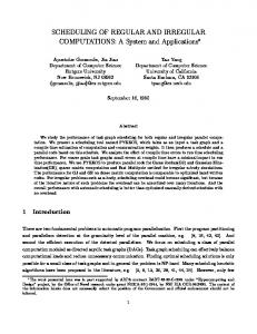
Figure 1: A bulk-synchronous parallel computation. nication network in a time unit. This interpretation of g indicates that, for an algorithm to be ecient, at least g local operations need to be performed for each data transfer. Accordingly, g can also be viewed as a measure of the throughput of the communication network. However, we prefer the de nition in [65], which relates g to the cost of realising a so-called h-relation. An h-relation is a communication pattern in which any processor sends and receives at most h items of data (or words); for conformity with the de nition of L, we will assume that the length of a word is that of a oating point data. Then, the cost of realising an h-relation is g maxfh; h0 g, where h0 is a threshold value accommodating the start-up cost of the communication. In other words, if h  h0 , the implementation of an h-relation costs gh. This result shows that in order to achieve ecient communication, the size of the exchanged messages must be large enough. The parameter g is also normalised with respect to s, i.e, it is expressed in ops per oating point word. As shown in [48], any parallel system can be regarded as a BSP computer, and represents a point in the (p; L; g) space of BSP computers. As we shall see in the following sections, it is exactly this abstraction from the hardware details of the machine that allows the development of portable and costable parallel software.

2.2 The BSP programming model

A BSP computation consists of a sequence of supersteps (Figure 1). The processors proceed asynchronously through each superstep, and barrier synchronise at the end of the supersteps|hence the name of \bulk-synchronous" parallel. Within a superstep, the processors are allowed to independently execute operations on locally held data and/or to initiate read/write requests for non-local data. However, the non-local memory accesses initiated during a superstep take eect only when all the processors reach the barrier synchronisation that ends that superstep. 7

The crucial bene t of this programming model is [65, 48] the separation of the three main components of a parallel application, namely computation, communication, and synchronisation. As a result, the cost of each of the three components can be independently and accurately assessed.

2.3 The BSP cost model

The BSP cost model is compositional: the cost of a BSP program is simply the sum of the costs of its constituent supersteps. Several expressions have been proposed for the cost of a single superstep. Thus, in [8], the authors adopted the expression

cost(i) = maxfL; wi ; ghi g for the cost of superstep i, 1  i  N of a N -superstep BSP program, where wi represents the maximum number of local operations executed by any processor during superstep i, and hi is the maximum number of words sent or received by any processor in superstep i. This formulation of the BSP cost accounts for a desired overlapping of computation and communication, and considers one of the synchronisation mechanisms proposed in [65], namely that in which the system checks the termination of a superstep every L time units. A more conservative alternative is [26] to charge a cost of maxfL; wi + ghi g for the execution of superstep i of a BSP computation. This cost is consistent with the fact that real parallel computers are often unable to fully overlap computation and communication. Indeed, as pointed out in [49], on many computers the most costly communication operation is the transfer of data from the operating system to the application buers, and this operation typically requires processor participation. Since a specialised mechanism for processor synchronisation is seldom available on the existing parallel computers, barrier synchronisations are usually implemented through inter-processor communication. As a consequence, it is often the case that the situation in Figure 1 arises, i.e., that the cost of synchronisation must be charged in addition to the computation and communication costs. Accordingly, the cost of superstep i, 1  i  N is in this case

cost(i) = L + wi + ghi ;

(1)

with L representing a measure of the latency of the communication network. It is this expression of the cost of a superstep that we will use throughout this report. However, it is worth noticing that all the expressions of the BSP cost presented in this section are equivalent within a small multiplicative constant, and the consistent use of any of them would lead to similar results. So far we considered that, irrespective of the value of hi |the maximum number of words sent or received by any processor during superstep i|the contribution of communication to the cost of superstep i is ghi . This is apparently against the requirement that 8

h must be greater than or equal to a threshold value h0 for the cost of an h-relation to be gh. The explanation is that the parameter L is large enough to cover for the start-up cost of an h-relation (i.e., L  gh0 ). Therefore, it is always safe to consider that the realisation of an h relation within a superstep brings a contribution of gh to the cost of

that superstep. The standard way of assessing the eciency of parallel algorithms is to compare them with the best (known) sequential algorithm that solves the same problem. The same strategy applies to BSP algorithms. Assume for instance that the sequential cost of solving a problem of size n is T (n), and the cost of an N -superstep BSP algorithm solving the same problem is

NL +

N X i=1

wi + g

N X i=1

hi = N (n; p)L + W (n; p) + gH (n; p):

Several ways of evaluating the eciency of BSP algorithms have been proposed so far. In [48], a BSP algorithm is considered to be ecient if W (n; p) = T (n)=p, and N (n; p) and H (n; p) are as small as possible. Also, in [26], two performance metrics,  = pW (n; p)=T (n) and  = gH (n; p)=(T (n)=p) are de ned, and a BSP algorithm is regarded as optimal if  = 1 + o(1) and  = o(1) or   1. We will assess the optimality of the BSP schedules devised in this report in a very similar way. Thus, we will say that a BSP schedule is k-optimal in computation if pW (n; p)=T (n) = k + o(1). For each schedule with N (n; p)=W (n; p) = o(1) and H (n; p)= W (n; p) = o(1), we will also strive to nd a threshold n0 such that for n  n0 , W (n; p)  maxfN (n; p)L; gH (n; p)g (a computation cost which is a order of magnitude larger than the communication and synchronisation overheads will be viewed as sucient for practical purposes). Whenever this is possible, we will say that the schedule is k-optimal for n  n0 , and expect to obtain a p=k speedup for a practical implementation of the schedule.

2.4 The development of BSP applications

Two methods of developing a BSP application have been envisaged in [65]. The rst method, called automatic mode programming, consists of writing the program in a PRAM style (i.e., without explicitly addressing the memory and communication management issues) and simulating the resulting code onto the target BSP computer. Optimallyecient BSP simulations of PRAMs have been devised [65, 66] for this purpose. The second method, called direct mode programming allows the programmer to retain control of memory and communication management. As emphasised in [65], the latter approach \avoids the overheads of automatic memory management and may exploit the relative advantage in throughput of computation over communication that may exist". Despite the solid theoretical results underlying PRAM simulation, practical BSP implementations of PRAM simulation are still in their infancy. Direct BSP algorithms and applications, on the other hand, have been extremely successful from the very early days of the BSP model. Besides the simplicity of designing and analysing direct BSP algorithms, this success is also due to the appearance of several very powerful environments for the development of portable BSP software. These environments include the 9

Oxford BSP Library [50] and the Green BSP Library [29], culminating with the recent proposal [30] and implementation of a BSP Worldwide standard library called BSPlib. All these libraries comprise a limited number of functions that can be called from C, Fortran, and other imperative languages with a similar memory model. Furthermore, the libraries have been implemented on a large number of parallel architectures, using native or generic primitives available on these machines.

2.5 BSP pseudocode

The sequential code whose mapping on a BSP computer is approached in this report, as well as the resulting BSP schedules are described in pseudocode. This subsection presents the conventions used in our pseudocode. First, for the sake of brevity, variables will not be explicitly declared. We will implicitly assume that loop indices are integers, whilst other variables and array elements will be assumed to be of oating point type, unless otherwise speci ed. Second, indentation will be used to indicate block limits instead of begin/end or similar constructs. Finally, less important and simple parts of a schedule will be described informally rather then being speci ed in detail. Three broad classes of statements will be used to describe a piece of code: assignments, conditional statements, and repetitive statements. All three types of statements have the same interpretation as in a typical imperative programming language, such as C or Fortran. The generic form of an assignment statement is variable = expression

where expression is an expression whose type coincides with that of the variable on the left-hand side of the assignment. A conditional statement has the generic form: if condition then statement else statement

where condition is a boolean condition, and the else part is optional. Two types of repetitive statements are used, the rst one to describe sequential loops: for index =lower bound,upper bound do statement

and the second to describe parallel loops: forall index =lower bound,upper bound do in parallel statement

Finally, we will use the constructs BSP start superstep and BSP end superstep to mark the beginning and the end of supersteps when describing BSP code. 10

S2(y ;y ;::: ;yK ) 1

2

read write

S1(x ;x ;:::;xK ) 1

2

read write | S1(x ;x ;:::;xK ) S2(y ;y ;:::;yK ) S1(x ;x ;:::;xK )  S2(y ;y ;:::;yK ) S1(x ;x ;::: ;xK ) o S2(y ;y ;::: ;yK ) 1

1

2

1

2

1

2

2

1

1

2

2

Table 1: The type of the dependence between two statement instances (at least one of which modi es the memory location accessed by both instances) depends only on the type of accesses to the commonly used variable, and on their execution order. In this table, the lexicographical order of the index vectors is (x1 ; x2 ; : : : ; xK ) < (y1 ; y2 ; : : : ; yK ).

3 Data dependence analysis and code transformation 3.1 Data dependence analysis

Three types of data dependence between two statement instances (the term `instance' refers to an actual execution of a statement in the program; if a statement belongs to a loop body and is executed many times, each such execution is considered a dierent instance of that statement) may prevent them from being concurrently executed (Figure 2):  true dependence (or ow dependence), when one of the statement instances reads a variable earlier modi ed by the other;  antidependence, when one of the statement instances uses the value of a variable which is later written by the other statement instance;  output dependence, when both statement instances write the same memory location. In each of the three cases, any legal transformation of the original program must preserve the order in which the two statement instances are executed (exceptions such as the output dependence of two statement instances that assign the same value to a variable, etc. are not discussed here). As shown in Table 1, the type of a data dependence depends only on the order and type of accesses made to the commonly used location of memory. There is also a control dependence that may exist between two statement instances, namely when the execution of one statement is conditioned by the result of evaluating the other. However, such dependences may be systematically converted to data dependences [2], and therefore no separate consideration of control dependences is necessary. Numerous tests, varying from simple and approximate [5, 72] to complex and exact [56] have been devised to identify whether two array references address the same memory location. Whenever an approximate test fails to prove independence, dependence is unconditionally assumed. Prior to its usage for the extraction of potential parallelism from the analysed sequential code, the dependence information acquired as a result of this analysis is \encoded" in a concise form. Three representations of this information are most popular: 11

S1: S2:

for i1 =1,n1-1 do for i2 =0,n2-2 do a[i1 ,i2 ]=... ...=f(a[i1-1,i2+1])

(a) true dependence: the value of a[x1 ; x2 ] modi ed by the instance of S1 for (i1 ; i2 ) = (x1 ; x2 ) is later used by the instance of S2 for (i1 ; i2 ) = (x1 + 1; x2 ? 1). This data dependence is denoted S1(x ;x )  S2(x +1;x ?1) . 1

S1:

2

1

2

for i=0,n-2 do a[i] = f(a[i+1])

(b) antidependence: the value of a[x] read by the instance of S1 for i = x is later written by the instance of S1 for i = x + 1. The notation used for this type of data dependence is S1(x)  S1(x+1) . S1: S2:

for i1 =0,n1 -1 do for i2 =1,n2 -1 do a[i1 ,i2 ]=... a[i1 ,i2 -1]=...

(c) output dependence: the variable a[x1 ; x2 ] is rst written by the instance of S1 for (i1 ; i2 ) = (x1 ; x2 ), then by the instance of S2 for (i1 ; i2 ) = (x1 ; x2 + 1). The output dependence is denoted S1(x ;x ) o S2(x ;x +1) . 1

2

1

2

Figure 2: Three types of data dependence ((a){(c)) may require that two statement instances are executed in a xed order in any legal transformation of a given program. A generic dependence between two statement instances S1(x ;x ;:::;xK ) and S2(y ;y ;:::;yK ) is denoted S1(x ;x ;:::;xK )  S2(y ;y ;:::;yK ) (i.e.,  =  +  + o ). 1

1

2

1

2

1

2

2

 The statement dependence graph [3] is a directed graph representation of the data

dependences. In this graph, each statement belonging to the analysed loop body is assigned a vertex, and each dependence relation between two statement instances is codi ed as an edge joining the vertices associated with the two statements. The edges are labeled with the level of the innermost loop for which the dependence still holds; this is the minimal information needed to decide whether a given statement may be vectorised from a certain loop level inwards.  The distance vector [39] and the direction vector [72] representations of data dependences store instead of several individual dependences only the dierence between the index vectors, respectively the relations (i.e., ` 1 is the level of the loop nest to be scheduled, and q  K is the number of distance vectors encoding the data dependences of the loop. The iterative schedule of a uniform-dependence loop nest which obeys the above mentioned constraint (possible after an ane transformation) is presented in Figure 9. The (K ? 1)-dimensional iteration space of the innermost loops of the loop nest is partitioned into p hypercubic tiles of size n=p1=(K ?1)  n=p1=(K ?1) 


 n=p1=(K ?1) , and in any iteration of the outermost loop, processor i, 0  i < p is assigned the computation of tile Tt ;t ;:::;tK , t2 p(K ?2)=(K ?1) + t3p(K ?3)=(K ?1) +


+ tK = i. After performing the computation of the loop body for the iteration points in the assigned tile, each processor sends the data involved in external data dependences (i.e., the halo data ) to the appropriate neighbour processor(s). Each iteration of the outermost loop takes one superstep, so the whole schedule requires n computation supersteps (as well as an initial \start-up" superstep in which loop-external input data is fetched by the processors). In each of the n supersteps of the schedule, the computation is perfectly distributed among the p processors, so the amount of computation per superstep is (nK ?1 c)=p; where c is the cost of computing the loop body for a single point of the iteration space. The maximum amount of data received or sent by any processor during a superstep is given by the following corollary to Theorem 4. 2

3

Corollary 8 The maximum amount of data sent or received by a processor in any superstep of the BSP schedule in Figure 9 is

2 3 K  n X 4 nK ?1 Y 5 ? Comm = 1=(K ?1) ? j dj j = p p d2D 0j=2 K 1 K ?2 X X n = (K ?2)=(K ?1) @ j dj j +o(1)A ; p d2D j =2

46

(17)

x=p^(1/(K-1)) for i1 =0,n-1 do forall t2 =0,x-1 do in parallel ............ forall tK =0,x-1 do in parallel Processor t2 *x^(K-2)+t3*x^(K-3)+...+tK: BSP begin superstep compute tile Tt2 ;t3 ;:::;tK : for i2 =t2 *n/x,(t2+1)*n/x-1 do ............ for iK =tK *n/x,(tK+1)*n/x-1 do

loop body

send halo data BSP end superstep

Figure 9: The iterative schedule of a uniform-dependence loop nest. where D is the set of distance vectors encoding the ow data dependences of the scheduled loop. Proof Theorem 4 gives the maximum amount of data to be sent by a processor after computing a K -dimensional rectangular tile of size x1  x2 


 xK . Considering this result for x1 = 1 and x2 = x3 =


= xK = n=p1=(K ?1) , and taking into account that tiles with dierent t1 coordinates, but identical t2 , t3 , : : : , tK coordinates are computed by the same processor, the quantity in (17) is obtained as an upper bound for the amount of data sent by a processor in any superstep of the BSP schedule. For the second part of the theorem, consider a distance vector d 2 D, and a generic processor Px that is assigned the computation of tile Tt ;t ;:::;tK in each of the n supersteps of the schedule. Then, for any superstep i1 , 0  i1 < n, only the tile computed by processor Px in superstep i1 + d1 will depend on data computed in superstep i1 and linked by data dependences encoded by d. The argument in Theorem 4 can be used to prove that the amount of data received by processor Px due to these data dependences is again 2

3

 K  n nK ?1 ? Y 1=(K ?1) ? j dj j ; p j =2 p where the rst term represents the volume of tile Tt ;t ;:::;tK , and the second is the volume of that part of the tile for which the data dependences encoded by d are solved internally. Summing this quantity over all distance vectors in D, and recalling that Px is a generic processor, Comm is indeed an upper bound for the amount of data received by any 2

3

processor during a superstep of the schedule.

2

The results obtained so far show that the cost of a single outermost loop iteration of 47

the schedule in Figure 9 is

L+

nK ?1c p

0

K K ?2 XX + g (K ?n2)=(K ?1) @ j dj p j =2 d2D

1 j +o(1)A ;

where D is the set of distance vectors representing the ow data dependences of the loop. Accordingly, the cost of the whole schedule is

0

1

K K ?1 K XX nL + np c + g p(K ?n2)=(K ?1) @ j dj j +o(1)A : d2D j =2

(18)

This cost is 1-optimal if it is dominated by the computation cost, i.e., if

9 8  K = < pL 1=(K ?1) gp1=(K ?1) X X j d j ; n  max : c j ;: c d2D j=2

(19)

Comparing this result with the cost of the uniform-dependence loop nest schedules developed in Section 5.4 (equations (11), (13)), it is immediate to see that the schedule devised in this section is preferable whenever its higher synchronisation overhead is not signi cant. As shown by relation (19), this condition is likely to be ful lled when K > 2 and the problem size is large, or even when K = 2 if the BSP parameter L is low, and the problem size is very large.

Example 7 Let us consider again the 2-level uniform-dependence loop nest in Example 6 for i1 =0,n-1 do for i2 =0,n-1 do a[i1 ,i2 ]=f1 (a[i1 -1,i2 ]) b[i1 ,i2 ]=f2 (a[i1 ,i2 ],b[i1 -1,i2 -2])

and use the schedule in Figure 9 for its mapping onto a BSP computer. Here is the resulting BSP schedule: for i1 =0,n-1 do forall t2 =0,p-1 do in parallel Processor t2 : BSP begin superstep for i2 =t2 *n/p,(t2+1)*n/p-1 do a[i1 ,i2 ]=f1 (a[i1 -1,i2 ]) b[i1 ,i2 ]=f2 (a[i1 ,i2 ],b[i1 -1,i2 -2]) if t2 1 can be evaluated to a function no more complex than f , and when f : Rk ! R is a linear transformation. In the former case, an 1-optimal BSP schedule can be obtained as follows. First, a0 is broadcasted to the p processors organised in a d-ary logic tree, d = L=g at a cost of 2L logd p [65]. Then, in a single computation superstep, each processor j , 0  j < p computes f jn=p in O(log(jn=p)) time, evaluates a[jn=p] = f jn=p(a0 ) in O(1) time, and, nally, computes a[i], jn=p < i < (j +1)n=p using the basic de nition of the recurrence in cn=p time. The total cost of this computation superstep is nc ; = (1 + o (1)) O(log n) + O(1) + nc p p giving a total cost of the entire schedule of

L(2 logL=g p + 1) + (1 + o(1)) nc p:

This cost is 1-optimal if n  2pL=c. 49

(20)

To obtain a BSP schedule for the evaluation of a k-level linear recurrence, we will use P the strategy proposed in [31]. Thus, if f (a[i?1]; a[i?2]; : : : ; a[i?k]) = kj=1 x[k ?j ]a[i?j ], we build the k  k (recurrence) matrix

0 BB 0 : : : 0 M=B B@ I

1

x[0] x[1] C CC .. .

x[k ? 1]

CA

(21)

with I the (k ? 1)  (k ? 1) identity matrix, and compute a[i], jn=p  i < jn=p + k on processor j , 0  j < p using the alternative de nition (a[jn=p] a[jn=p + 1] : : : a[jn=p + k ? 1]) = (a[0] a[1] : : : a[k ? 1])
Mjn=p: The BSP schedule comprises two stages. In the rst stage, the values of a[i], x[i], 0  i < k are broadcasted to all processors. Using the standard broadcasting strategy, the cost of this stage is (L + 2kg). Then, in the second stage, each processor j , 0  j < p computes Mjn=p in (k3 log(jn=p)) time, evaluates a[i], jn=p  i < jn=p + k using the alternative de nition in (21) in (k2 ) time, then computes a[i], jn=p + k  i < (j + 1)n=p in kn=p time. Accordingly, the cost of the entire schedule is

nk ; =  ( L + 2 kg ) + (1 + o(1)) (L + 2kg) + (k3 log n) + (k2 ) + nk p p which is 1-optimal for

(22)

n  (L + 2kg)p=k:

5.7 Scheduling regular computations involving broadcasts

There is a very important loop structure which, although stands for a regular pattern of computation, has data dependences that cannot be expressed as distance vectors. This is because certain items of loop-computed data are repeatedly used for the computation of the loop body at many iteration points. Since its mapping on a distributed-memory computer typically requires broadcasts of the multiple-used items of data, we will call this loop structure a broadcast loop nest. As shown in Figure 11, a generic K -level broadcast loop nest, K > 1 comprises a number of so-called broadcast initialisation loops, and a main computation loop which iteratively computes the elements of a (K ?1)-dimensional output array a. Each of the s > 0 broadcast initialisation loops has the structure in Figure 12, and computes broadcast data used by the following execution of the main computation loop. Some of the broadcasts within the main computation loop may be based on data computed by its previous execution (i.e., ak [i2 ; : : : ; ij ?1 ; fk (i1 ); ij +1 ; : : : ; iK ] = a[i2 ; : : : ; ij ?1 ; fk (i1 ); ij +1 ; : : : ; iK ] for some 1  k  s), and the corresponding broadcast initialisation loops are then missing. In such a case, an additional auxiliary array ak and a broadcast initialisation loop can be added to bring the broadcast loop nest to the \normalised" form in Figure 11. 50

for i1 =0,n-1 do broadcast init loop 1 broadcast init loop 2 ............... broadcast init loop s for i2 =0,n-1 do .............. for iK =0,n-1 do a[i2 ,...,iK]=f(a[i2,...,iK],...,ak[i2 ,...,ij?1,fk (i1 ),ij+1 ,...,iK],...)

Figure 11: A K -level broadcast loop nest. for i2 =0,n-1 do ............... for ij?1 =0,n-1 do for ij+1 =0,n-1 do ............... for iK =0,n-1 do ak [i2 ,...,ij?1,fk (i1 ),ij+1 ,...,iK]=...

Figure 12: The k-th broadcast initialisation loop in Figure 11, 1  k  s. Although in Figure 11 all the loops iterate from 0 to n ? 1, this is not essential for the results devised in this section; the only purpose of this initial assumption was to simplify the description of a broadcast loop nest. In fact, the BSP schedules presented in the remainder of this section do not even require that the iteration space be rectangular. Before approaching the scheduling of a generic broadcast loop nest, let us analyse several well-known examples of this structure. First, in Figure 13, the pseudocode of triangular linear system solving is arranged to match the notations used for a generic 2-level broadcast loop nest. The triangular linear system to be solved is Ca1 = a, C = (ci i )0i i 2L logL=g p; : 2 L + g npxK?  ; otherwise j for any iteration of the outermost loop of L. Proof For any xed value taken by (i2 ; : : : ; ij?1 ; ij+1; : : : ; iK ) within the iteration space of the main computation loop of L, the value of ak [i2 ; : : : ; ij ?1 ; fk (i1 ); ij +1 ; : : : , iK ] is 1

required for the computation of the n iteration points on the segment determined by this xed value and by 0  ij < n. Since the iteration space is partitioned into tiles whose size along the j -th direction is xj , the iteration points on this segment are assigned to n=xj of the p processors. Accordingly, for any xed value taken by (i2 ; : : : ; ij ?1 ; ij +1 ; : : : ; iK ), n=xj processors need the value of ak [i2 ; : : : ; ij?1 ; fk (i1 ); ij+1 ; : : : ; iK ] for the computation of their tiles. In fact, our straightforward schedule ensures that ak [i2 ; : : : ; ij ?1 ; fk (i1 ); ij +1 ; : : : ; iK ] is computed by one of these n=xj processors (namely by that processor whose tile comprises the iteration point (i2 ; : : : ; ij ?1 ; fk (i1 ); ij +1 ; : : : ; iK )). As a consequence, for any xed value taken by (i2 ; : : : ; ij ?1 ; ij +1 ; : : : ; iK ), an item of data must be broadcasted to exactly n=xj ? 1 processors, if xj < n, or to no processor at all otherwise. As this result proves the theorem for the case when xj = n, we shall consider that xj < n in the remainder of this proof. To compute the maximum number of data items to be broadcasted by any processor during an iteration of the outermost loop of L, we need to nd the maximum number of dierent values taken by (i2 ; : : : ; ij ?1 ; ij +1 ; : : : ; iK ) across a tile. It is immediate to see that this number Q is a constant equal to x2 : : : xj?1xj+1 : : : xK . Using the load balancing constraint Kl=2 xl = nK ?1=p, the number of dierent items of data to be sent by any processor involved in the computation of the k-th broadcast initialisation loop is (nK ?1=p)=xj = nK ?1 =(pxj ). Finally, since the iteration space of the main computation loop of L is partitioned along the directions given by i2 , : : : , ij ?1 , ij +1 , : : : , iK with K ? 2 hyperplanes parallel to the broadcast direction, the number of items of data to be received by any processor which is not a sender is again nK ?1=(pxj ). To summarise, the p processors can be viewed as partitioned into nK ?2=(x2 : : : xj ?1 xj+1 : : : xK ) groups of n=xj processors, with one of the processors in each group having to broadcast exactly nK ?1=(pxj ) items of data to all other processors in its group. The most ecient way of implementing the broadcast depends on the value of K . Thus, for K = 2, there is only one item of data to be broadcasted by one of the processors to the other p ? 1 processors, and the algorithm in [65] is to be used. This algorithm realises the broadcast by sending the data to the p ? 1 processors in a d-ary tree fashion, with d = L=g; the total cost of the broadcast is 2L logd p. For K > 2 on the other hand, nK ?1=(pxj )  n=xj for any practical values of n and p, and the standard two-superstep broadcast procedure is used independently for each group of processors. In the rst superstep of this procedure, the sender partitions the 54

data to be broadcasted into n=xj ? 1 chunks of equal size, and sends a dierent chunk of data to each of the other processors in its group. Then, in the second superstep, each processor sends its chunk of data to all the other processors in the group. Both supersteps have the same cost L + gnK ?1 =(pxj ), and the result in (23) is proved.

2

The result provided by the previous theorem allows us to choose the appropriate tiling, and to compute the cost of the second stage of an iteration of the BSP schedule. Thus, if there is any direction l, 2  l  K such that no broadcast data is used along direction l, then the best partition is that with xl = n=p, and xj = n if j 6= l because this tiling implies no communication costs at all; the cost of an iteration of the schedule is in this case K ?1 L + n p c + (nK ?2); because stage 2 does not exist, and the other two stages of each iteration can be executed in a single superstep. Furthermore, since the computations performed by dierent processors are fully independent, the whole computation can be executed in a single superstep, and the total cost of the schedule is K

L + np c (1 + o(1)):

This cost is 1-optimal, provided that the problem size is large enough for the computation cost to dominate the synchronisation overhead, i.e., that

 pL 1=K

n c

:

If there are several directions that correspond to no broadcast, any tiling which has

xj = n for all broadcast directions j , and respects the load balancing constraint QKj=2 xj = nK ?1=p has the above cost. The optimal tiling is then the one which minimises the cost of

the initialisation superstep, i.e., of the superstep in which the pure-input data is fetched. Nevertheless, in most practical situations, broadcast loop nests comprise data broadcasts along each of the K ? 1 directions of the main computation loop. As this is by far the most common case, we will assume that a single broadcast stream exists for each of these K ? 1 directions. Since the s = K ? 1 broadcasts are independent, the communication cost of the second stage of an iteration of the BSP schedule is given by the sum of the communication costs of the K ? 1 broadcasts. As for the synchronisation cost, it is the same as for a single broadcast, because the K ? 1 broadcasts can be performed concurrently, in two supersteps. Consequently, if K > 2, the cost of the second stage is K 1 K ?1 X : 2L + 2 gn

p

j =2 xj

According to the mean inequality, this cost is minimised for x2 = x3 =


= xK = n=p1=(K ?1) ; its minimum value is K ?2 2L + 2g n (K ? 1) :

p(K ?2)=(K ?1) 55

When this tiling is used, and the rst superstep of stage 2 is merged with the only superstep of stage 1, the cost of a whole iteration of the schedule becomes K ?2 K ?1 3L + n p c + (nK ?2) + 2g n(K ?2)(K=(K??1) 1) ; p giving a total cost of the schedule of K ?1 K 3nL + np c (1 + o(1)) + 2g n(K ?2)(K=(K??1) 1) :

(24)

p

Accordingly, 1-optimality is obtained in the general case if the computation cost dominates equation (24), i.e., if the problem size is large enough:

( 1=(K ?1) 1=(K ?1) ) 3 pL 2 g ( K ? 1) p n  max : ; c

c

So far, we considered that the iteration space of the main computation loop is rectangular, and were able to achieve 1-optimality due to a perfect load balancing. Unfortunately, the basic schedule does not preserve this perfect load balancing when the iteration space of the main computation loop is not rectangular. To overcome this limitation, the partitioning of the iteration space of the main computation loop must be modi ed as follows. For any direction of the iteration space along which the number of iteration points varies during the computation, the tiles are interleaved along that direction. Informally, interleaving the tiles along the j -th direction of the iteration space, 2  j  K means changing the size of the tiles along the j -th direction from xj to xj =j , where j > 1 is the interleaving factor. More than p tiles result after all interleavings, and tile Tc ;c ;:::;cK is assigned to the processor which would execute tile Tc mod n=x ;c mod n=x ;:::;cK mod n=xK in the basic schedule. An example of interleaving for a 3-level broadcast loop nest is presented in Figure 16. As shown in Figure 16, the number of processors along any direction of the iteration space does not change after the interleaving. Consequently, the interleaving does not modify the broadcast costs. The load balancing, however, is greatly improved: roughly speaking, an interleaving factor of j along a direction j reduces the imbalance7 along that direction j times. Ideally, one would choose j = n=xj to minimise the imbalance. In practice however, it is better to choose a smaller value for the interleaving factors (e.g., j = 10::20) because such a value yields an acceptable load balancing, while still enabling the exploitation of data locality (by the caching system, for instance). 2

2

2

3

3

3

5.7.2 Broadcast loop nest scheduling through broadcast elimination

Let us consider again the generic form of a K -level broadcast loop nest in Figure 11, and assume that fk (i1 ) = 0 (or, in the general case, fk (i1 ) = lj , where the loop indexed by ij

the imbalance of a computation is de ned as the ratio between the maximum deviation from the average processor workload and the average processor workload 7

56

i3

i3

i3

0

2

1

0

3

2

1

0

3

2

i2

0

1

0

1

2

3

2

3

0

1

0

1

2

3

2

3

1

3

i2

(a) initial tiling

(b) interleaving along direction i 2

i2 (c) interleaving along both direction i 2 and direction i 3

Figure 16: Tile interleaving for a 3-level broadcast loop nest. The tiles obtained after the standard partitioning (a) are interleaved along direction i2 (b), then along direction i3 (c); the index of the processor assigned to each tile is marked on the tile. The interleaving factors 2 = 3 = 2 were used. The tiling in (b) can be used to schedule Gauss-Jordan elimination, as the iteration space shrinks along direction i2 in this case, while the tiling in (c) is appropriate for Gauss elimination, whose iteration space shrinks both in direction i2 and in direction i3 . is the missing loop from the k-th broadcast initialisation loop, and lj is the lower bound of the iteration space along direction ij ) for any 1  k  s. Then, the k-th broadcast initialisation loop can be rewritten as in Figure 17, and the s broadcast initialisation loops can be fusioned with the main computation loop. Assuming that the initial broadcast loop nest comprises broadcasts along all directions of the iteration space, the equivalent loop nest which results is a fully permutable loop nest whose data dependences are encoded by the set of distance vectors D = f(d1 ; d2 ; : : : ; dK ) j (9j : 1::K  dj = 1) ^ (8j 0 : 1::K  (j 0 6= j ) ) (dj0 = 0))g. This fully permutable loop nest can then be scheduled as shown in Section 5.4; if the rst enhanced schedule in this section is used, the total cost of the resulting BSP code is

n L + (1 + o(1)) nK c + (1 + o(1)) g(K ? 1)nK ?1 ; x p p(K ?2)=(K ?1)

P

P

(25)

since in this particular case d2D Kj =1?1 dj = K ? 1. Comparing this cost with the one in (24), it is immediate to notice that both schedules are computationally optimal, but have dierent synchronisation and communication costs. Thus, the communication cost of the schedule based on broadcast elimination is only half the communication cost of the schedule using broadcast implementation. Although typically negligible for both schedules, it 57

for i2 =0,n-1 do ............... for ij?1 =0,n-1 do for ij =0,n-1 do for ij+1 =0,n-1 do ............... for iK =0,n-1 do if ij =0 then ak [i2 ,...,ij?1,ij ,ij+1 ,...,iK]=... else ak [i2 ,...,ij?1,ij ,ij+1 ,...,iK]=ak [i2 ,...,ij?1,ij

? 1,ij+1,...,iK]

Figure 17: Rewriting a broadcast initialisation loop to eliminate broadcasts when fk(i1 )=0. is worth pointing out that the synchronisation cost is also smaller for the broadcast elimination schedule. Consequently, the schedule devised in this section is preferable to the broadcast implementation schedule, especially when the iteration space to be scheduled is rectangular. For non-rectangular iteration spaces, however, the application of the schedule based on broadcast implementation may result in better balanced parallel programs, so the usage of the technique devised in Section 5.7.1 is worth considering. If there is any broadcast initialisation loop k, 1  k  s for which fk (i1 ) 6= 0 (or, in the general case, fk (i1 ) 6= lj , where the loop indexed by ij is the missing loop from the broadcast initialisation loop k, and lj is the lower bound of the iteration space along direction ij ), it is still possible to eliminate the broadcasts. This can be achieved by rewriting the k-th broadcast initialisation loop as shown in Figure 18, with two distinct loop nests replacing the original broadcast initialisation loop. Furthermore, each of the other broadcast initialisation loops as well as the main computation loop must be splitted into two loop nests whose iteration spaces coincide with those of the loop nests in Figure 18. After all the broadcast initialisation loops are converted into (K ? 1)-level loop nests (those with fk (i1 ) = 0 into a single loop nest, and those with fk (i1 ) 6= 0 into two loop nests), all the loop nests with identical iteration spaces are fusioned.0 Finally, the outermost loop nest is distributed to the resulting loop nests yielding 2s K -level fully permutable loop nests, where s0 , 0  s0  s represents the number of broadcast initialisation loops for which fk (i1 ) 6= 0. The set of iteration spaces corresponding to the resulting fully permutable loop nests represents a partitioning of the iteration space of the original loop nest into equally sized chunks. These loop nests can then be executed in the appropriate order, using one of the scheduling techniques in Section 5.4. If the rst load balancing improving technique is used, the total cost of the resulting schedule is " Kc K ?1 # n g ( K ? 1) n 0 n s : (26) L + (1 + o(1)) + (1 + o(1)) 2

x

p(K ?2)=(K ?1)

p

The total cost is 2s0 times higher than that in (25) because the 2s0 fully permutable loop nests must be executed in a well-de ned order, one after another. As a result, the 58

for i2 =0,n-1 do ............... for ij?1 =0,n-1 do for ij =fk [i1 ],n-1 do for ij+1 =0,n-1 do ............... for iK =0,n-1 do if ij =0 then ak [i2 ,...,ij?1,ij ,ij+1 ,...,iK]=... else ak [i2 ,...,ij?1,ij ,ij+1 ,...,iK]=ak [i2 ,...,ij?1,ij 1,ij+1 ,...,iK] for i2 =0,n-1 do ............... for ij?1 =0,n-1 do for ij =fk [i1 ]+1,0,-1 do for ij+1 =0,n-1 do ............... for iK =0,n-1 do ak [i2 ,...,ij?1,ij ,ij+1 ,...,iK]=ak [i2 ,...,ij?1,ij + 1,ij+1 ,...,iK]

?

Figure 18: Rewriting a broadcast initialisation loop to eliminate broadcasts when fk(i1 ) 6= 0. schedule which implements the broadcasts instead of eliminating them is recommended in this case.

5.8 BSP scheduling of hybrid skeletons

It is often the case that the loop structures which occur in real programs comprise features characteristic to two or more of the regular computation patterns whose BSP scheduling was approached in this chapter. When this happens, the best schedule which exploits these features|possibly a schedule which combines elements belonging to several of the techniques described so far|has to be used. This section presents the most common hybrid loop structures which can be encountered in imperative programs, and discusses their scheduling onto a BSP computer.

5.8.1 Fully parallel outermost loops with reduction innermost loops

Two of the most basic building blocks in imperative programs dealing with dense data structures are matrix-vector multiplication and matrix-matrix multiplication. While optimal BSP algorithms for these basic operations have already been developed (see for instance [48]), the existence of many other instances of the same pattern of computation makes the study of its BSP scheduling worthwhile. It is not dicult to see that the main computation of the standard matrix-matrix multiplication algorithm (Figure 19) is a 3-level tightly-nested loop comprising two fullyparallel outermost loops and a reduction innermost loop. Accordingly, the scheduling 59

for i1 =0,n-1 do for i2 =0,n-1 do for i3 =0,n-1 do c[i1 ,i2 ]=c[i1,i2 ]+a[i1,i3 ]*b[i3,i2 ]

Figure 19: Matrix-matrix multiplication: C = A
B. techniques corresponding to both loop structures can be employed to schedule this loop nest. Thus, the iteration space of the two outermost loops can be partitioned as shown in Section 5.2, with the resulting tiles being computed in a single computation superstep; this strategy yields the straightforward BSP schedule described in [48, 65]. Second, one can leave the outermost loops sequential and schedule the n2 reductions for parallel execution as shown in Section 5.3. Although computation-optimal, this strategy is highly inecient, mainly due to the very large synchronisation overhead. Nevertheless, the best schedule for matrix-matrix multiplication is a combination of the two techniques mentioned so far. This schedule, described in [48], requires 2 computation supersteps. In the rst computation superstep, each processor executes the loop body for the iteration points in an equally-sized hypercubic tile of the loop nest. The partial results obtained in this superstep are then combined in the second computation superstep to generate the global result. Generalising this schedule, which mixes elements characteristic to both fully-parallel loop nest scheduling and reduction scheduling, Ding and Stefanescu [18] have devised a technique for the ecient scheduling of generic loop nests with the same structure. The scheduling technique proposed in [18] is brie y described in Section 4.3.

5.8.2 Iteration spaces partially spanned by the distance vector set Another common hybrid loop structure is the loop nest with fully parallelisable outermost loops, and the innermost loops forming a uniform-dependence loop nest whose distance vectors span its entire iteration space. Typically, such a loop structure is induced by a uniform-dependence loop nests whose distance vectors span the iteration space of the loop only partially. Indeed, if a K -level uniform-dependence loop nest has only k, 0 < k < K linearly independent distance vectors, then an ane transformation exists that maps the iteration space of the loop to an iteration space in which the distance vectors have null elements along k directions of the iteration space. Consequently, the k loops of the transformed loop nest that correspond to these directions can be made outermost loops and executed in parallel [4]. Once again, techniques corresponding to two loop structures can be employed to schedule such a loop nest. First, one can consider only the outermost k loops of the loop nest, and schedule the whole loop as a fully parallel loop nest. Also, one may schedule the innermost K ? k loops as indicated in Sections 5.4 and 5.5, leaving the outermost loops sequential, or attempting to parallelise their execution at the same time. Among these various choices, the former strategy is by far the simplest. Since it also leads to optimal schedules for common problem sizes (see Section 5.2) it is recommended in all circumstances. 60

6 BSP scheduling of generic loop nests This chapter discusses the scheduling of loop nests that match none of the regular patterns of computation whose BSP scheduling has been approached in Chapter 5. The results presented in this chapter build on the work of Kuck [38, 39], and of Allen and Kennedy [3]. However, in approaching the scheduling of a generic loop nest, we add new theoretical results that generalise those in [3, 38, 39], and permit the identi cation of that kind of parallelism which is best suited for the BSP setting. The BSP scheduling of a generic, untightly-nested loop comprises three stages. In the rst stage, a data-dependence graph which is an enhanced version of that proposed in [3] and brie y described in Section 3.1 is built. Then, in a second stage, the information in this dependence graph is used to identify the potential parallelism of the loop nest. Finally, in a third stage, the resulting potential parallelism is scheduled for parallel execution on a BSP computer.

6.1 The enhanced data-dependence graph of a generic loop nest

In this section, we describe the structure of the enhanced data-dependence graph of a generic loop nest, and provide the theoretical background for the identi cation of the potential parallelism of the loop nest using the information in this graph. Each of the theoretical results introduced in this section will be illustrated with several simple examples. Sometimes, keeping these examples as simple as possible will make them match one of the regular patterns of computation analysed in Chapter 5. Clearly, this resemblance does not invalidate the generality of the new results, or their applicability to the parallelisation of generic loop nests. Throughout the section we will consider a generic loop nest L whose statements are Si, 1  i  N , and whose loop indices ij , 1  j  K , iterate from 0 to nj ? 1. However, L need not be a perfect loop nest, i.e., we allow the body of any loop to comprise both other loops and/or statements. The loops of L are labeled with natural numbers between 1 and K . This labeling is done in such a way that any set of perfect nested loops are assigned consecutive numbers, and, if the labels of two loops are 1  x < y  K , then loop x cannot belong to the body of loop y. With the above de ned notations, the enhanced data-dependence graph of L is a directed graph G comprising a vertex for each of the N statements of L, and an edge between each pair of statements Sx, Sy , 1  x; y  N for which the non-existence of any dependence Sx  Sy cannot be proved. Each vertex of G is assigned a label Sj (L), where Sj is the statement represented by that vertex, and L represents the ordered set of loops surrounding statement Sj . Each edge of G is also assigned a label  (S; P ), where  2 f; ; o g represents the type of the dependence, and the signi cance of S and P is explained later in this section. We will start with a theorem which summarises results from [3].

Theorem 10 (Allen and Kennedy [3]) Let Sx and Sy be two (not necessarily distinct) statements of a generic loop nest L which are surrounded by k  1 common loops 61

indexed by i1 ; i2 ; : : : ; ik . Suppose that a data dependence Sx Sy must be assumed between the two statements due to the fact that both statements use the m-dimensional array a (or, if Sx = Sy , due to the fact that a is both read and modi ed by the statement): Sx : Sy :

...a[f(i1,i2 ,...,ik)]... ...a[g(i1,i2 ,...,ik)]...

with f; g : Zk ! Zm. Then, if for some value 2 1::k, and for any legal values (x1 ; x2 ; : : : ; xk ) < (y1 ; y2 ; : : : ; yk ) assigned to (i1 ; i2 ; : : : ; ik ),

(x1 ; x2 ; : : : ; x ) = (y1 ; y2 ; : : : ; y ) ) f (x1 ; x2 ; : : : ; xk ) 6= g(y1 ; y2 ; : : : ; yk )

(27)

and, if > 1, it cannot be proved that

(x1 ; x2 ; : : : ; x ?1 ) = (y1 ; y2 ; : : : ; y ?1 ) ) f (x1 ; x2 ; : : : ; xk ) 6= g(y1 ; y2 ; : : : ; yk );

(270 )

the sequential execution of the outermost loops surrounding Sx and Sy satis es all the restrictions imposed by this data dependence on the execution order of the iteration space of L, and is called the upper nesting level of the data dependence8 . Proof Consider two generic iteration points (x1; x2 ; : : : ; xk ) < (y1 ; y2; : : : ; yk ) such that

f (x1 ; x2 ; : : : ; xk ) = g(y1 ; y2 ; : : : ; yk ): The original loop nest executes these two iterations in lexicographical order, i.e., rst (x1 ; x2 ; : : : ; xk ), then (y1 ; y2 ; : : : ; yk ). Consequently, any rewriting of the loop which preserves this execution order satis es the restrictions imposed by the considered data dependence. Assume now that the outermost loops surrounding Sx and Sy are executed sequentially, and (some of) the other loops are executed concurrently. Then, according to the hypothesis of the theorem, (x1 ; x2 ; : : : ; x ) must be lexicographically smaller than (y1 ; y2 ; : : : ; y ). Hence, iteration (x1 ; x2 ; : : : ; xk ) is executed before iteration (y1 ; y2 ; : : : ; yk ), and the new execution order of the iteration space of L satis es the restrictions imposed by the data dependence Sx  Sy .

2

The name of upper nesting level given to from (27) is justi ed by the fact that the associated data dependence can be viewed as \eliminated" when the outermost loops surrounding the two statements involved in the dependence are left sequential. Theorem 10 provides a strategy for the parallelisation of the innermost loops of a loop nest.

Example 8 For the untightly-nested loop 8



is called the nesting level of the data dependence in [3]

62

for i1 =0,n1 -1 do a[i1 ]=f(i1) for i2 =0,n2 -1 do S2: b[i1,i2 ]=g(a[i1],i2) S1:

forall i1 =0,n1 -1 do in parallel a[i1 ]=f(i1) forall i2 =0,n2-1 do in parallel S2: b[i1 ,i2 ]=g(a[i1],i2 ) S1:

a

b

Figure 20: A loop nest comprising a loop-independent ow dependence S1 S2 (a), and the potential parallelism of the loop (b). for i1 =0,n1 -1 do for i2 =0,n2 -1 do S1: a[i1 ,i2 ]=f(i1 ,i2 ) for i3 =0,n3 -1 do S2: b[i1 ,i2 ,i3 ]=g(a[i1 -1,i2 ],i3 )

a ow data dependence S1 S2 of upper nesting level 1 exists because

8(x1 ; x2 ); (y1 ; y2) : 0::n1 ? 1  0::n2 ? 1  x1 = y1 ) (x1 ; x2 ) 6= (y1 ? 1; y2 ); and

8(x1; x2 ); (y1 ; y2 ) : 0::n1 ? 1  0::n2 ? 1  (x1 ; x2) 6= (y1 ? 1; y2 )

cannot be proved to be true. Accordingly, the loop can be rewritten as for i1 =0,n1 -1 do forall i2 =0,n2 -1 do in parallel S1: a[i1 ,i2 ]=f(i1 ,i2 ) forall i3 =0,n3 -1 do in parallel S2: b[i1 ,i2 ,i3 ]=g(a[i1 -1,i2 ],i3 )

with the potential parallelism of the loop revealed. An extreme case which must be addressed separately is that of a loop-independent data dependence. Indeed, for a loop-independent dependence, relation (27) does not hold for any value 2 1::k. Therefore, in this extreme case we will take = 1, indicating that the dependence is not eliminated however many loops surrounding the two statements are left sequential. It is immediate to see, however, that all the loops surrounding two statements involved in a loop-independent dependence can be executed in parallel without aecting the correctness of the transformed code. An example of a loop nest comprising a loop-independent dependence is presented in Figure 20. The following theorem is complementary to Theorem 10: it de nes the lower nesting level of a data dependence, and provides a way of using this new parameter of a dependence for the extraction of the coarse-grained potential parallelism of a generic loop nest. 63

Theorem 11 Let Sx and Sy be two (not necessarily distinct) statements of a generic loop nest L which are surrounded by k  1 common loops indexed by i1 , i2 , : : : , ik . Suppose

that a data dependence Sx Sy must be assumed between the two statements due to the fact that both statements use the m-dimensional array a (or, if Sx = Sy , due to the fact that a is both read and modi ed by the statement): Sx : Sy :

...a[f(i1,i2 ,...,ik)]... ...a[g(i1,i2 ,...,ik)]...

with f; g : Zk ! Zm. Then, if for some value  2 1::k, and for any legal values (x1 ; x2 ; : : : ; xk ) < (y1 ; y2 ; : : : ; yk ) assigned to (i1 ; i2 ; : : : ; ik ) it cannot be proved that

(x1 ; x2 ; : : : ; x ) 6= (y1 ; y2 ; : : : ; y ) ) f (x1 ; x2 ; : : : ; xk ) 6= g(y1 ; y2 ; : : : ; yk );

(28)

and, if  > 1,

(x1 ; x2 ; : : : ; x?1 ) 6= (y1 ; y2 ; : : : ; y?1 ) ) f (x1 ; x2 ; : : : ; xk ) 6= g(y1 ; y2 ; : : : ; yk );

(280 ) the sequential execution of the innermost k ?  + 1 loops surrounding Sx and Sy satis es all the restrictions imposed by this data dependence on the execution order of the iteration space of L, and  is called the lower nesting level of the data dependence. Proof As in the proof of Theorem 10, consider two generic iteration points (x1 ; x2; : : : ; xk ) < (y1; y2 ; : : : ; yk ) such that

f (x1 ; x2 ; : : : ; xk ) = g(y1 ; y2 ; : : : ; yk ): Again, any rewriting of the loop which executes (x1 ; x2 ; : : : ; xk ) and (y1 ; y2 ; : : : ; yk ) in lex-

icographical order satis es the restrictions imposed by the considered data dependence. Assume now that the outermost  ? 1 loops surrounding Sx and Sy are executed concurrently, and all the other k ?  + 1 loops are left sequential. Then, according to the de nition of  (equation (28)), (x1 ; x2 ; : : : ; x?1 ) = (y1 ; y2 ; : : : ; y?1 ), and both iterations of interest are executed in the same iteration of outermost parallel loops. The order in which they are executed is imposed by the lexicographical order of (x ; x+1 ; : : : ; xk ) and (y ; y+1 ; : : : ; yk ). Obviously, since (x1 ; x2 ; : : : ; xk ) < (y1 ; y2 ; : : : ; yk ) and (x1 ; x2 ; : : : ; x?1 ) = (y1 ; y2 ; : : : ; y?1 ), we must have (x ; x+1 ; : : : ; xk ) < (y ; y+1 ; : : : ; yk ), so the two iteration points are executed in the correct order.

2

Example 9 Here is an example of a 2-level loop nest comprising a ow data dependence

S1S1 of lower nesting level  = 2:

for i1 =0,n1 -1 do for i2 =0,n2 -1 do S1: a[i1 ,i2 ]=f(a[i1 ,i2

? 1])

Then, according to Theorem 11, the outermost loop of the nest can be executed in parallel: 64

forall i1 =0,n1 -1 do in parallel for i2 =0,n2 -1 do S1: a[i1 ,i2 ]=f(a[i1 ,i2 1])

?

The potential parallelism of the transformed loop can be readily scheduled for execution on a BSP computer, yielding a 1-superstep BSP program. It is worth emphasising that, since the upper nesting level of this loop is = 2, the method described in [3] and summarised by Theorem 10 is not able to identify any parallelism in the loop. Furthermore, although a loop interchange would enable the application of the parallelisation strategy in [3], it will only expose the ne-grained parallelism in the loop, leading to a n2 -superstep BSP program. The lower nesting level of a data dependence can be regarded as the maximum value

 such that the sequentialisation of loop  and of the innerer loops \breaks" (i.e., elim-

inates) the data dependence. Accordingly, the lower nesting level of a loop-independent dependence is considered to be  = 0. Indeed, not even the sequentialisation of all loops surrounding two statements involved in a loop-independent data dependence breaks the dependence. The last theorem presented in this section provides a way of increasing the granularity of the potential parallelism extracted from a generic loop nest, as well as a method for the identi cation of parallel loops situated between the lower and the upper nesting level of a data dependence.

Theorem 12 Let Sx and Sy be two (not necessarily distinct) statements of a generic loop nest L which are surrounded by k  1 common loops indexed by i1 , i2 , : : : , ik . Assume that a data dependence Sx  Sy exists between the two statements due to the fact that both statements use the m-dimensional array a (or, if Sx = Sy , due to the fact that a is both read and modi ed by the statement): Sx : Sy :

...a[f(i1,i2 ,...,ik)]... ...a[g(i1,i2 ,...,ik)]...

with f; g : Zk ! Zm. Let P  1::k be the set of all loops j , 1  j  k, with the property that, for any legal values (x1 ; x2 ; : : : ; xk ) < (y1 ; y2 ; : : : ; yk ) assigned to (i1 ; i2 ; : : : ; ik ),

xj 6= yj ) f (x1 ; x2 ; : : : ; xk ) 6= g(y1 ; y2 ; : : : ; yk ):

(29)

Then, some or all the loops in P (which is called the set of fully parallel loops of the data dependence) can be made outermost loops and executed in parallel without violating the restrictions imposed by the considered data dependence on the execution order of the iteration space of L. Proof Assume that the loop nest L is rewritten such that some (or all) the loops in P are made outermost loops and executed in parallel. We will prove the theorem by showing that any pair of iteration points (x1 ; x2 ; : : : ; xk ) < (y1 ; y2 ; : : : ; yk ) for which f (x1 ; x2 ; : : : ; xk ) = g(y1 ; y2 ; : : : ; yk ), is executed in the correct, lexicographical order by

65

the transformed loop. To do so, it is enough to notice that, for any loop j 2 P , xj = yj for any pair of interdependent iteration points. Consequently, any two interdependent iteration points are executed in the same iteration of the outermost parallel loops, and in a order imposed by the lexicographical order of the elements of the two index vectors that correspond to the other loops. Since only equal elements are \eliminated" from the two index vectors, this is exactly the lexicographical order of the iteration points, and the proof is complete.

2

It is worth noticing that, with the notations in Theorem 12, the set of fully parallel loops of a loop-independent data dependence is P = 1::k. Indeed, all the loops surrounding two statements involved in a loop-independent data dependence can be parallelised as long as the order of the two statements within the loop body is preserved. The three parameters of a data dependence introduced so far are not redundant. In order to prove this, we will present several examples of simple loop nests whose parallelisation cannot be achieved without the usage of the two new parameters,  and P . First, let us compare the parameters  and . From their de nitions in (28) and (27), respectively, it is immediate to see that, for any data dependence,   . The ow data dependence S1 S1 in the following loop nest is an example of a data dependence whose lower nesting level is actually lower than its upper nesting level: for i1 =0,n1 -1 do for i2 =0,n2 -1 do for i3 =0,n3 -1 do S1: a[i1 ,i2 ,i3 ]=f(a[i1 ,i3 ,i3

? 1])

In this case, the lower nesting level of the data dependence is  = 2 because x1 6= y1 ) (x1 ; x2 ; x3 ) 6= (y1 ; y3 ; y3 ? 1) for any values assigned to (x1 ; x2 ; x3 ), (y1 ; y2 ; y3 ), and it cannot be proved that (x1 ; x2 ) 6= (y1 ; y2 ) ) (x1 ; x2 ; x3 ) 6= (y1 ; y3 ; y3 ? 1). The upper nesting level of the data dependence, on the other hand, is = 3, since (x1 ; x2 ; x3 ) = (y1 ; y2 ; x3 ) ) (x1 ; x2 ; x3 ) 6= (y1 ; y3 ; y3 ? 1), and it cannot be proved that (x1 ; x2 ) = (y1 ; y2 ) ) (x1 ; x2 ; x3 ) 6= (y1 ; y3 ; y3 ? 1) for any legal value assigned to (x1 ; x2 ; x3 ), (y1 ; y2 ; y3 ). Hence, we have 2 =  < = 3, and the outermost loop of the loop nest can be executed in parallel: forall i1 =0,n1 -1 do in parallel for i2 =0,n2 -1 do for i3 =0,n3 -1 do S1: a[i1 ,i2 ,i3 ]=f(a[i1 ,i3 ,i3 1])

?

Finally, P , the set of fully parallel loops of a data dependence, adds new useful information to that conveyed by  and . Indeed, although 1::( ? 1)  P , P can also comprise other loops, as it does for the ow data dependence S1 S1 in the following loop for i1 =0,n1 -1 do for i2 =0,n2 -1 do S1: a[i1 ,i2 ]=f(a[i1 -1,i2 ])

66

In this case,  = = 1, and P = f2g, showing that the inner loop can be brought into the outermost position and parallelised: forall i2 =0,n2 -1 do in parallel for i1 =0,n1 -1 do S1: a[i1 ,i2 ]=f(a[i1 -1,i2 ])

Since the usage of  and alone would only permit the parallelisation of the loop indexed by i2 as the innermost loop, the introduction of P is justi ed. At a rst glance, it might seem that P = 1::( ? 1) [ ( + 1)::k. This is not true, as illustrated by the following example: for i1 =0,n1 -1 do for i2 =0,n2 -1 do for i3 =0,n3 -1 do for i4 =0,n4 -1 do S1: a[i1 ,i2 ,i3 ,i4 ]=f(a[i2 ,i2 ,i3 -1,i4 +1])

The ow data dependence S1 S1 in this example has  = 1, = 3, and P = f2g. Consequently, the loop between the lower and the upper nesting levels of the dependence (i.e., the loop indexed by i2 ) can be brought to the outermost position and parallelised, while the loop indexed by i +1 can only be parallelised in the innermost position. In conclusion, although the three parameters of a data dependence are related, each of them conveys dierent dependence information. Furthermore, the parameters and P must be determined independently, whereas the parameter  can be deduced from the value of P : 8 > if P = 1::k < 0;  = > 1; if 1 2=P : + 1; if 1::  P ^ + 1 2=P So far, we have introduced three parameters characterising a data dependence between two statements that access the elements of the same array within the body of a generic loop nest. In doing so, we assumed that various comparisons of the subscripts selecting the array elements used by the two statements can be performed. However, we have provided no clue about how these comparisons can actually be realised. This is because we are not proposing any new method for the assessment of the truth of propositions (27)-(270 ), (28)-(280 ), or (29). Nevertheless, several ways of doing these comparisons, such as the greatest common divisor (GCD) test [3] or the Banerjee inequality test [5], do exist, and can be used in conjunction with the new results devised in this section. The remainder of this section describes how the information provided by the three parameters of a data dependence is incorporated into the enhanced data-dependence graph G of a generic loop nest. The straightforward way of integrating the parameters of a data dependence into G would be to simply make them part of the label assigned to the edge corresponding to the considered data dependence. However, this is only possible for the set of fully parallel loops of a data dependence P . This is because no labeling of the loops of a generic loop nest L exists which would permit the interpretation of the lower 67

S1: S2: S3:

for i1 =0,n1-1 do for i2 =0,n2-1 do a[i1 ,i2 ]=f1 (i1 ,i2 ) for i3 =0,n3 -1 do b[i1 ,i2 ,i3 ]=f2(a[i1 ,i2 ],b[i1+1,i2+1,i3 ],c[i2,i2 -1,i3]) c[i1 ,i2 ,i3 ]=f3(b[i1 -1,i2-1,i3 +2])

Figure 21: Example of a untightly-nested loop.

and upper nesting levels of all the data dependences of L in a consistent manner. Indeed, in the general case, it is impossible to label the loops of a generic loop nest in such a way that any pair of statements is surrounded by loops which are assigned consecutive numbers. In fact, as illustrated by the following example, this is impossible to achieve even for very simple loop nests: for i1 =0,n1 -1 do for i2 =0,n2 -1 do S1 S2 for i3 =0,n3 -1 do S3 S4

In this example, the three loops cannot be labeled in such a way that both statements S1; S2 , and statements S3 ; S4 are surrounded by consecutively numbered loops. As a result, when assessing the lower and upper nesting levels of the dependences between S1 and S2 , and between S3 and S4 , one has to assume a dierent labeling of the three loops. Since this requirement renders the resulting lower and upper nesting levels of a dependence dependent on the dependence itself, a way of coherently expressing the information encapsulated in the two parameters is needed. The solution adopted by the enhanced dependence graph introduced in this section is to represent this information as the set of loops that must be kept unchanged for the considered data dependence to be satis ed. This set, which is the complementary of P , is denoted S , and comprises all the loops situated between the lower and the upper nesting levels of the considered dependence, and which are not in P .

Example 10 An example of a more complex generic loop nest, and its associated en-

hanced dependence graph are depicted in Figure 21 and Figure 22, respectively. As illustrated by the dependence S1 S2 in this example, the set S of a loop-independent data dependence comprises no loop at all. Also, some of the loops surrounding the statements involved in a data dependence may belong neither to S , nor to P ; for the ow dependence S2 S3 for instance, 2; 3 2= S [ P .

68

S1 (1,2) ({},{1,2}) ({1,2},{3})

({1},{3})

({1},{})

S2 (1,2,3)

S3 (1,2,3)

({1,2},{3})

Figure 22: The enhanced dependence graph of the loop nest in Figure 21.

6.2 Potential parallelism identi cation in a generic loop nest

In this section, an algorithm for the identi cation of the potential parallelism available in a generic loop nest is introduced. This algorithm is an extension of the loop distribution algorithm of Kuck [38], and of the parallel code generation algorithm of Allen and Kennedy [3]. The main advantages of the new algorithm are the usage of the enhanced data-dependence graph of the loop nest for the extraction of more parallelism, and the fact that it exposes the coarse-grained parallelism in the loop nest rather than the ne-grained one. The latter advantage, crucial in the BSP setting where ne-grained parallelism may translate into prohibitive synchronisation overheads, is, to our knowledge, unique among the parallelisation algorithms proposed so far. The algorithm is based on the following corollary to Theorems 10-12.

Corollary 13 Let L be a generic loop nest and G its associated enhanced data-dependence graph. Assume that the n  1 edges of G are labeled j (Sj ; Pj ), with 1  j  n, and that S = [nj=1Sj and P = \nj=1Pj . Then, if  the loops indexed by ij , j 2 P are brought into the outermost position and executed in parallel;

 the loops indexed by ij , j 2 S are left unchanged;  the loops indexed by ij , j 2= S [ P are executed in parallel, the restrictions imposed by all the data dependences of L are not violated. Proof For any data dependence j , 1  j  n, the parallel version of the loop nest

proposed by the corollary keeps all the loops in Sj sequential, and brings to the outermost position only loops in Pj . Hence, according to the results in Theorems 10, 11 and 12, the restrictions imposed by all the n data dependences of L are satis ed.

2

Example 11 Figure 23 illustrates the usage of the corollary. The loop nest depicted in

Figure 23(a) comprises three ow data dependences. First, statement S3 uses a value computed by statement S1 in the same iteration of the common surrounding loops, so a loop-independent dependence S1 S3 exists; this dependence is labeled (S1 ; P1 ), with S1 = fg and P1 = f1; 2g (Figure 23(b)). Second, statement S2 uses a value computed by statement S1 in a previous iteration, so a loop-carried data dependence S1 S2 with 69

S1: S2: S3:

for i1 =0,n1 -1 do for i2 =0,n2 -1 do for i3 =0,n3-1 do a[i1 ,i2 ,i3 ]=f1 (b[i1,i2 ,i3 -1]) b[i1 ,i2 ,i3 ]=f2 (a[i1-1,i2,i3 -1]) c[i1,i2 ]=f3(a[i1 ,i2 ,n3 -1])

(a) ({1},{2})

S1 (1,2,3)

({3},{1,2})

S2 (1,2,3)

({},{1,2})

S3 (1,2)

S1: S2: S3:

(b)

forall i2 =0,n2-1 do in parallel for i1 =0,n1 -1 do for i3 =0,n3-1 do a[i1 ,i2 ,i3 ]=f1 (b[i1,i2 ,i3 -1]) b[i1 ,i2 ,i3 ]=f2 (a[i1-1,i2,i3 -1]) c[i1,i2 ]=f3(a[i1 ,i2 ,n3 -1])

(c) Figure 23: A generic loop nest (a), its associated enhanced data-dependence graph (b), and the potential parallelism exposed by Corollary 13 (c).

 = = 1 (and hence with S2 = f1g) and P2 = f2g exists. Finally, the elements of array b modi ed by statement S2 are used in a later iteration by statement S1 ; a ow data dependence with  = = 3 (i.e., with S3 = f3g) and P = f1; 2g exists between the two statements. Consider now S = S1 [S2 [S3 = f1; 3g and P = P1 \P2 \P3 = f2g. Then, according to Corollary 13, the three dependences are satis ed when the loop indexed by i2 is brought into the outermost position and executed in parallel, and the other two loops are left unchanged, so the parallel version in Figure 23(c) is correct. This parallel version reveals enough coarse-grained parallelism for the loop nest to be executed in a single superstep on a BSP computer. However, it is worth emphasising that Corollary 13 does reveal insucient or, indeed, no parallelism at all in some cases. Consider for instance the following example of a loop nest: 70

S1: S2:

for i1 =0,n1 -1 do for i2 =0,n2 -1 do a[i1 ,i2 ]=f1 (a[i1 -1,i2 ]) b[i1 ,i2 ]=f2 (a[i1 ,i2 -1])

This loop nest comprises two data dependences, S1 S1 with  = = 1 and P1 = f2g, and S1 S2 with  = = 2 and P2 = f1g. Obviously, since S = S1 [ S2 = f1; 2g and P = fg, the application of Corollary 13 identi es no potential parallelism in the loop nest. However, the following parallel version of the loop nest is correct: S1:

S2:

forall i2 =0,n2 -1 do in parallel for i1 =0,n1 -1 do a[i1 ,i2 ]=f1 (a[i1 -1,i2 ]) forall i1 =0,n1 -1 do in parallel forall i2 =0,n2 -1 do in parallel b[i1 ,i2 ]=f2 (a[i1 ,i2 -1])

When such cases occur, the loop nest cannot be parallelised as a whole, but must be broken into separate parts which are parallelised independently. Before presenting an algorithm which, in addition to applying Corollary 13, realises this partitioning of the loop nest whenever necessary, let us make very clear what the parallel program designer expects from such an algorithm. Consider the following example of a loop nest, in which the problem size n is much greater than p, the number of processors of the BSP computer. for i1 =0,n-1 do S1 for i2 =0,n-1 do S2 for i3 =0,n-1 do S3

The sequential cost of executing the loop nest is O(n3 ), so what one expects from a pprocessor BSP version of this loop nest is an execution cost of O(n3 =p). Obviously, this can only be obtained if the execution of statement S3 |which is called the main statement of the loop nest|is parallelised. Furthermore, the fact that statements S1 and S2 are executed in parallel or not is irrelevant for the successful parallelisation of the loop nest as a whole. Consequently, a parallelisation algorithm must concentrate on the identi cation of potential parallelism corresponding to the main statements of a loop nest, possibly neglecting the less signi cant parts of the loop. A second feature that must characterise a good parallelisation algorithm is illustrated by the following loop nest: for i1 =0,n-1 do for i2 =0,2 do for i3 =0,n-1 do S1

71

Assuming again that the problem size n is much greater than the number of processors p, any successful BSP version of this loop nest must be able to concurrently execute the loop body for dierent iteration points along direction(s) i1 or/and i3 of the iteration space. Indeed, a parallelisation of the loop indexed by i2 is of little use in this case. Therefore, a parallelisation algorithm must focus on those loops whose iteration space size depends on the problem size|these are called the main loops of the loop nest|rather than on the loops whose index bounds are (small) constants. Finally, assume that a main statement S of a loop nest is surrounded by several main loops which iterate from 0 to n ? 1, where n is the problem size, and suppose that one of these main loops can be parallelised. As emphasised throughout this section, the relative level of the parallel loop among the other main loops is of crucial importance. If the parallel loop is in the innermost position (i.e., has the relative level 1), a synchronisation is required after every n executions of the statement S . As a result, the BSP program induced by this parallelisation could be ecient only if the problem size is much greater than the synchronisation cost L, which is a very restrictive constraint. If, on the other hand, the parallel loop has the relative level 2 (i.e., it is in the second innermost position), barrier synchronisations are only required after each n2 (parallel) computation steps. Hence, an ecient BSP program can be obtained for n2  L, which is a much more relaxed constraint. Accordingly, when attempting to identify the potential parallelism of a loop nest, one must also pay attention to the relative level of the loops that are parallelised. The observations made so far are taken into account by the parallelisation algorithm in Figure 24. This algorithm identi es the potential parallelism of a generic loop nest using the information in its enhanced data-dependence graph G . In doing so, the algorithm attempts to parallelise the execution of all statements in the main statement set Stmts, which is provided as a second parameter to the algorithm. A statement in Stmts is considered to be successfully parallelised when (at least) one of its surrounding main loops can be executed in parallel, and the relative level of this loop is greater than or equal to a threshold level th level provided as input to the algorithm. The set of the main loops of the loop nest (denoted Loops) is also a parameter of the algorithm. The algorithm works as follows. In a rst stage, the algorithm attempts to parallelise the loop nest as a whole by applying Corollary 13 to the data-dependence graph G received as the rst parameter. The resulting parallel version of the loop nest is accepted|and the algorithm terminates|if each statement from Stmts is successfully parallelised. The algorithm also terminates when the loop nest comprises a single statement, since in this case no partitioning of the loop is possible. When none of the two termination conditions is ful lled, the algorithm enters a second stage, in which the partitioning of the loop nest is attempted. First, the -blocks (i.e., the maximal cycles or individual vertices belonging to no cycle [3, 39]) of G are identi ed. Then, if G comprises a single -block, the cyclic dependence of this -block is broken by applying Theorem 10 to a data dependence belonging to the cycle and whose elimination requires that a minimum number of loops are kept sequential. Clearly, one should always try to eliminate a data dependence that requires the sequentialisation of loops not in Loops. Once the cyclic dependence is broken, the edge corresponding to the eliminated 72

G

proc parallelise( , Stmts, Loops, th level) Stage 1.Parallelise the loop nest as a whole apply Corollary 13 to if comprises a single vertex then STOP if any statement in Stmts is surrounded by at least a parallel loop of relative level greater than or equal to th level from Loops then STOP Stage 2.Partition the loop nest and parallelise the resulting parts partition into  -blocks if comprises a single  -block then break the cyclic dependence by sequentialising the minimum number of loops adjust and Loops to account for the changes call parallelise( , Stmts, Loops, th level) else lexicographically sort the  -blocks in lexicographical order, call parallelise recursively for each  -block

G

G

G

G

G

G

Figure 24: Potential parallelism identi cation algorithm. data dependence is deleted from G , and the parallelisation algorithm is applied recursively to the resulting data-dependence graph. Finally, when G comprises many -blocks, these -blocks are lexicographically ordered, and the parallelisation procedure is recursively called for each -block. In order to apply the algorithm to an individual -block, the reduction of G to the set of statements belonging to the block, and the relevant sets of statements Stmts and main loops Loops are computed in the straightforward way. Then, a call to the parallelisation procedure with the new set of parameters is issued.

Example 12 To illustrate the usage of the parallelisation algorithm, let us identify the potential parallelism of the loop nest in Figure 21 by calling

G ; Stmts; Loops; th level)

parallelise(

with G the enhanced data-dependence graph in Figure 22, Stmts = fS2 ; S3 g, Loops = f1; 2; 3g, and th level = 2. In the rst stage of the algorithm, the application of Corollary 13 yields S = [3j =1Sj = f1; 2g and P = \3j =1Pj = fg, so only the loop indexed by i3 can be parallelised in the innermost position: S1: S2: S3:

for i1 =0,n1 -1 do for i2 =0,n2 -1 do a[i1 ,i2 ]=f1 (i1 ,i2 ) forall i3 =0,n3 -1 do in parallel b[i1 ,i2 ,i3 ]=f2 (a[i1 ,i2 ],b[i1 +1,i2 +1,i3 ],c[i2 ,i2 -1,i3 ]) c[i1 ,i2 ,i3 ]=f3 (b[i1 -1,i2 -1,i3 +2])

73

Since for all the statements in Stmts the relative level of the parallel loop is 1 < th level = 2, the main statements of the loop nest are not successfully parallelised, and the algorithm proceeds to Stage 2. In this stage, the data-dependence graph G is partitioned into two -blocks, one comprising the vertex S1 and no edge, and the other comprising the cycle formed by vertices S2 and S3 . Next, the parallelisation procedure is called recursively for the two -blocks:

G ; fg; f1; 2g; 2) G ; fS2 ; S3g; f1; 2; 3g; 2)

parallelise( 1 parallelise( 2

where G1 and G2 represent the reductions of the data-dependence graph G to the two blocks. The parallelisation of the rst -block succeeds in Stage 1, because this -block comprises a single vertex; the parallel version of this part of the loop nest is: S1:

forall i1 =0,n1 -1 do in parallel forall i2 =0,n2 -1 do in parallel a[i1 ,i2 ]=f1 (i1 ,i2 )

For the second -block, however, Stage 1 is again unable to reveal enough parallelism: only the loop indexed by i3 is parallelised in the innermost position. As a result, the re-partitioning of G2 is attempted in Stage 2 of the algorithm. Since G2 comprises a single -block, a new partition is not possible, so the algorithm attempts to break the cyclic dependence. Obviously, the data dependence whose elimination requires the sequentialisation of a minimum number of loops is S2 S3 . Hence, this data dependence is eliminated by keeping the loop indexed by i1 sequential, and the parallelisation procedure is called recursively for the data-dependence graph ({2},{3})

S2 (2,3)

({2},{3})

S3 (2,3)

This time, the application of Corollary 13 parallelises the loop indexed by i3 in the outermost position, succeeding to reveal enough coarse-grained parallelism for the algorithm to terminate. The nal parallel version of the entire loop nest is: S1:

S2: S3:

forall i1 =0,n1 -1 do in parallel forall i2 =0,n2 -1 do in parallel a[i1 ,i2 ]=f1 (i1 ,i2 ) for i1 =0,n1 -1 do forall i3 =0,n3 -1 do in parallel for i2 =0,n2 -1 do b[i1 ,i2 ,i3 ]=f2 (a[i1 ,i2 ],b[i1 +1,i2 +1,i3 ],c[i2 ,i2 -1,i3 ]) c[i1 ,i2 ,i3 ]=f3 (b[i1 -1,i2 -1,i3 +2])

74

6.3 Scheduling the potential parallelism of a generic loop nest

Once the coarse-grained potential parallelism of a generic loop nest is identi ed, it must be scheduled for parallel execution on a BSP computer. This section discusses the underlying principles of a successful mapping of this potential parallelism on a BSP machine. First, the principal target of an ecient scheduling strategy must be the balanced distribution of the main statement executions among the p processors of the parallel computer. This goal can be achieved by considering the parallel loops surrounding each main statement, partitioning their iteration space into p equally sized tiles, and computing each such tile on a dierent processor. Second, since the communication overheads may grow high if the scheduling of each main statement of a loop nest is done independently, one has to correlate the scheduling of various main statements. This can be done by tiling only the iteration space of those parallel loops which induce an identical or similar distribution of the data used within the loop body. Consider the following example of a parallel version of a generic loop nest:

S1:

S2:

forall i1 =0,n-1 do in parallel forall i2 =0,n-1 do in parallel for i3 =0,n-1 do ...a[i1 ,i2 ,i3 ]... forall i2 =0,n-1 do in parallel forall i3 =0,n-1 do in parallel for i1 =0,n-1 do ...a[i1 -1,i2 ,i3 ]...

If the iteration space of the rst loop nest are tiled along directions i1 and i2 , and the iteration space of the second loop nest along directions i2 and i3 , the elements of array a need to be redistributed after the computation of the rst loop nest. Since in this case each processor has to exchange its block of n3 =p elements of a for another block of the same size, the communication cost of this data redistribution is gn3 =p. Clearly, this cost may well dominate the computation cost O(n3 =p), rendering the considered BSP schedule inecient. If, on the other hand, the iteration space of both loop nests is tiled along direction i2 alone, a similar distribution of array a results for the two loop nests. As this reduces the communication cost to gn2 , an ecient BSP schedule can thus be obtained. It is possible, however, that no tiling direction common to all the main statements of the considered loop nest exists. When this is the case, it is necessary to choose between the concurrent scheduling of all the main statements and the concurrent scheduling of only some of them. The decision must be made in accordance with the (communication) cost of the data redistribution required by the rst choice. As concerns the secondary statements of a loop nest, they should be scheduled in a way which preserves as much as possible the data distribution induced by the scheduling of the main statements. Consider for instance the following parallel version of a loop nest: 75

S1:

S2:

forall i1 =0,n-1 do in parallel forall i2 =0,n-1 do in parallel ...a[i1 ,i2 ]... forall i2 =0,n-1 do in parallel for i1 =0,n-1 do for i3 =0,n-1 do ...a[i1 ,i2 ]...

In this case, statement S2 must be scheduled by tiling the iteration space of the surrounding loops along direction i2 . This tiling induces a data distribution in which each of the p processors is assigned n=p columns of array a. To preserve this data distribution (thus avoiding additional communication costs), the iteration space of the rst loop must also be tiled along direction i2 of its iteration space. The extent to which the data distribution preservation must take precedence over other scheduling criteria is dicult to assess in the general case. Here is an example of a loop nest whose secondary statement scheduling must be based on the actual values of the BSP parameters for the target computer: S1:

S2:

forall i1 =0,n-1 do in parallel for i2 =0,n-1 do a[i1 ,i2 ]=f(a[i1 ,i2 -1]) forall i2 =0,n-1 do in parallel for i1 =0,n-1 do for i3 =0,n-1 do ...a[i1 ,i2 ]...

As in the previous example, the iteration space of the second loop nest must be tiled along direction i2 . This tiling yields a data distribution in which each processor is assigned n=p columns of the array a. This distribution can only be maintained for the rst 2-level loop nest if this loop nest is sequentialised, and the processors compute a n  n=p tile of its iteration space in p consecutive supersteps. The total cost of executing the rst loop nest in this way is pL+cn2 +gpn. An alternative to this strategy is to execute the rst loop nest concurrently, in the straightforward way, and then to redistribute the elements of array a. The cost of the resulting BSP schedule of the rst loop is L + cn2 =p + gn2 =p. Obviously, the less expensive strategy can only be decided at run time, when the parameters of the target BSP machine are known.

76

7 Conclusions and future work One of the major aims currently focusing the eorts of the parallel computing community is the development of a realistic basis for the design and programming of general purpose parallel computers. The advent of the bulk-synchronous parallel model has oered a solution to this problem, providing a possible underlying framework for the devising of both scalable parallel architectures and portable parallel software. Consequently, a huge amount of research work is now targeted at the standardisation of the newly emerged model, and especially at the development of a unanimously accepted set of BSP programming primitives [30]. Taking into account the present pace of progress in the latter pursuit, it is very likely that a universal, BSP-based platform for portable parallel application design will be agreed upon in the very near future. Notwithstanding the advantages of the direct, manual design of BSP algorithms and applications, one cannot neglect the existence of a broad basis of ecient sequential solutions for the most various classes of problems. If the huge amount of work invested into the development of this basis of sequential code is to be taken advantage of, then reliable techniques for the automatic mapping of sequential code onto a BSP computer are needed. A rst, important step in this direction has been made with the recent devising of eective techniques for the identi cation of the potential parallelism of a sequential program. As a result of this step, a virtual parallel version of a sequential program can be automatically generated. How to actually map this (PRAM-like) virtual parallelism onto a BSP computer is a question whose de nite answer is still to be found. A rst solution to this problem was proposed in [65, 66], where optimally-ecient BSP simulations of PRAMs were devised by exploiting parallel slackness and by using shared-memory address hashing. Simulation, however, places restrictive demands on the target BSP architecture, requiring [47] powerful multithreading support and fast context switching and address translation capabilities. Furthermore, even if parallel architectures providing these features were built, simulation could attain the lower bounds established for the execution of a virtual parallel program on a real parallel computer only when no locality whatsoever exists in the simulated code [58]. Since the lack of locality is a reality only for the computations involving complex, sparse data structures, simulation is very unlikely to ever represent a feasible generic solution for the mapping of potential parallelism on BSP computers. An alternative solution for this mapping is therefore worth seeking. It is such an alternative to PRAM simulation that the project whose rst steps are presented in this report proposes by considering the BSP scheduling of potential parallelism. Whereas hitherto scheduling has merely been used to derive architecture-speci c parallel programs or special-purpose parallel designs, no real impediment exists to its usage in the context of portable parallel code generation. Indeed, as shown in Chapter 5, regular patterns of computation can be successfully identi ed and eciently scheduled within the framework of the BSP model. Furthermore, the kind of potential parallelism required for the BSP scheduling of generic loop nests can be identi ed using the techniques presented in Chapter 6. Nevertheless, the work carried out so far only covers the initial phase of our project, 77

which aims at developing a coherent framework for bulk-synchronous parallel scheduling. Thus, further eorts will be dedicated to the integration of the observations in Section 6.3 into an algorithm for the the BSP scheduling of generic loop nests. Also, we intend to use the scheduling techniques devised so far for the development of a generic strategy for the BSP scheduling of virtual parallel programs, and, nally, to implement this strategy as a useful tool for the design of portable parallel software.

78

Acknowledgements The author would like to thank Prof. W.F. McColl for his advice and encouragement. I am also highly indebted to Dr. M.B. Giles for suggesting the rst load balancing improving technique described in Section 5.4.1 of the current report.

79

References [1] T.L. Adam et al. A comparison of list schedules for parallel processing systems. Communications of the ACM, 17:685{690, 1974. [2] J.R. Allen et al. Conversion of control dependence to data dependence. In Conference Record of the 10th ACM Symposium on Principles of Programming Languages, pages 177{189. ACM Press, 1983. [3] J.R. Allen and K. Kennedy. Automatic translation of Fortran programs to vector form. ACM Transactions on Programming Languages and Systems, 9(4):491{542, October 1987. [4] D F Bacon et al. Compiler transformations for high-performance computing. ACM Computing Surveys, 26(4):346{420, December 1994. [5] U. Banerjee. Dependence Analysis for Supercomputing. Kluwer Academic Publishers, 1988. [6] U. Banerjee. A theory of loop permutation. In Proceedings of the 2nd Workshop on Programming Languages and Compilers for Parallel Computing, 1989. [7] U. Banerjee. Unimodular transformations of double loops. In A. Nicolau, editor, Advances in Languages and Compilers for Parallel Processing, Research Monographs in Parallel and Distributed Computing. MIT Press, 1991. [8] R.H. Bisseling and W.F. McColl. Scienti c computing on bulk synchronous parallel architectures. Technical Report 836, Department of Mathematics, Utrecht University, December 1993. [9] P. Boulet et al. (Pen)-ultimate tiling? Integration, the VLSI Journal, 17(1):33{51, August 1994. [10] R. Calinescu. Bulk synchronous parallel algorithms for conservative discrete event simulation. Parallel Algorithms and Applications, 9:15{38, 1996. [11] R. Calinescu. Bulk synchronous parallel algorithms for optimistic discrete event simulation. Technical Report TR-8-96, Programming Research Group, Oxford University Computing Laboratory, April 1996. [12] R. Calinescu. Bulk synchronous parallel scheduling of uniform dags. In Luc Bouge et al., editors, Euro-Par'96. Parallel Processing, volume 2 of Lecture Notes in Computer Science 1124, pages 555{562. Springer{Verlag, 1996. [13] R. Calinescu and D.J. Evans. A parallel model for dynamic load balancing in clustered distributed systems. Parallel Computing, 20(1):77{91, January 1994.

80

[14] R. Calinescu and D. Grigoras. A neural self-organizing scheme for dynamic load allocation. In A. De Gloria et al., editors, Transputer Applications and Systems '94, pages 860{868. IOS Press, 1994. [15] T.L. Casavant and J.G. Kuhl. A taxonomy of scheduling in general-purpose distributed computing systems. IEEE Transactions on Software Engineering, 14(2):141{154, February 1988. [16] T. Cheatham et al. Bulk synchronuous parallel computing { a paradigm for transportable software. Technical Report TR-36-94, Center for Research in Computing Technology, Harvard University, Cambridge, Massachusetts, December 1994. [17] D. Culler et al. LogP: Towards a realistic model of parallel computation. In Proceedings of the 4th ACM SIGPLAN Symposium on Principles and Practice of Parallel Programming, pages 19{22. ACM Press, 1993. [18] Y.-Z. Ding and D. Stefanescu. Ecient scheduling of loop nests for BSP programs. Technical Report TR-04-95, Center for Research in Computing Technology, Harvard University, Cambridge, Massachusetts, 1995. [19] J. Dongarra and A.R. Hind. Unrolling loops in FORTRAN. Software Practice and Experience, 9(3):219{226, March 1979. [20] H. El-Rewini et al. Task Scheduling in Parallel and Distributed Systems. PTR Prentice Hall, 1994. [21] A.P. Ershov. ALPHA|an automatic programming system of high eciency. Journal of the ACM, 13(1):17{24, January 1966. [22] P. Feautrier. Some ecient solutions to the ane scheduling problem. part I, onedimensional time. International Journal of Parallel Programming, 21(5):313{348, October 1992. [23] P. Feautrier. Some ecient solutions to the ane scheduling problem. part II, multidimensional time. International Journal of Parallel Programming, 21(6):389{420, December 1992. [24] S. Fortune and J. Wyllie. Parallelism in random access machines. In Proceedings of the 10th Annual ACM Symposium on Theory of Computing, pages 114{118, 1978. [25] A. Gerasoulis and T. Yang. A comparison of clustering heuristics for scheduling DAGs on multiprocessors. Journal of Parallel and Distributed Computing, 14(4):276{ 291, December 1992. [26] A.V. Gerbessiotis and L.G Valiant. Direct bulk-synchronous parallel algorithms. Journal of Parallel and Distributed Computing, 22(2):251{267, August 1994. [27] A. Gibbons and P Spirakis, editors. Lectures on Parallel Computation. Cambridge International Series on Parallel Computation: 4. Cambridge University Press, 1993. 81

[28] L.A. Goldberg et al. An optical simulation of shared memory. In SPAA '94. 6th Annual ACM Symposium on Parallel Algorithms and Architectures, pages 257{267. ACM, 1994. [29] M. W. Goudreau et al. The Green BSP library. Technical Report CS-TR-95-11, Department of Computer Science, University of Central Florida, Orlando, 1995. [30] M. W. Goudreau et al. A proposal for the BSP Worlwide standard library. Technical report, BSP Worldwide Technical Report, April 1996. Available from http://www.bsp-worldwide.org/standard/. [31] A. C. Greenberg et al. Ecient parallel algorithms for linear recurrence computation. Information Processing Letters, 15(1):31{35, August 1982. [32] D. Grigoras and R. Calinescu. kernel service for dynamic load balancing. In B.M. Cook et al., editors, Transputer Applications and Systems '95, pages 269{279. IOS Press, 1995. [33] T.J. Harris. A survey of PRAM simulation techniques. ACM Computing Surveys, 26(2):187{206, June 1994. [34] K.T. Herley and G. Bilardi. Deterministic simulations of PRAMs on bounded degree networks. SIAM Journal of Computing, 23(2):276{292, April 1994. [35] F. Irigoin and F. Triolet. Supernode partitioning. In Conference Record of the 15th ACM Symposium on Principles of Programming Languages, pages 319{329. ACM Press, 1988. [36] H. Kasahara and S. Narita. Practical multiprocessor scheduling algorithms for ef cient parallel processing. IEEE Transactions on Computers, C-33(11):1023{1029, November 1984. [37] W. Kelly and W. Pugh. Finding legal reordering transformations using mappings. In K. Pingali et al., editors, Languages and Compilers for Parallel Computing, Lecture Notes in Computer Science 892, pages 107{124. Springer{Verlag, 1995. [38] D.J. Kuck. A survey of parallel machine organization and programming. ACM Computing Surveys, 9(1):29{59, March 1977. [39] D.J. Kuck. The Structure of Computers and Computations. John Wiley and Sons, 1978. [40] L Lamport. The parallel execution of do loops. Communications of the ACM, 17(2):83{93, February 1974. [41] C. Lengauer. Loop parallelization in the polytope model. In E. Best, editor, CONCUR'93, Lecture Notes in Computer Science 715, pages 398{416. Springer{Verlag, 1993. 82

[42] V. Leppanen and M. Penttonen. Work{optimal simulation of PRAM models on meshes. Nordic Journal of Computing, 2(1):51{69, Spring 1995. [43] W. Li and K. Pingali. A singular loop transformation framework based on nonsingular matrices. In Proceedings of the 5th Workshop on Languages and Compilers for Parallel Computers, pages 249{260, 1992. [44] A.W. Lim and M.S. Lam. Communication-free parallelization via ane transformations. In K. Pingali et al., editors, Languages and Compilers for Parallel Computing, Lecture Notes in Computer Science 892, pages 92{106. Springer-Verlag, 1995. [45] D.B. Loveman. Program improvement by source-to-source transformation. Journal of the ACM, 24(1):121{145, January 1977. [46] B.A. Malloy et al. Scheduling DAG's for asynchronous multiprocessor execution. IEEE Transactions on Parallel and Distributed Systems, 5(5):498{508, May 1994. [47] W F McColl. General purpose parallel computing. In A. Gibbons and P. Spirakis, editors, Lectures on Parallel Computation, Cambridge International Series on Parallel Computation: 4, pages 337{391. Cambridge University Press, 1993. [48] W.F. McColl. Scalable computing. In J. Van Leeuwen, editor, Computer science today : recent trends and developments, Lecture Notes in Computer Science 1000, pages 46{61. Springer-Verlag, 1995. [49] R. Miller. Two approaches to architecture-independent parallel computation. PhD thesis, Oxford University Computing Laboratory, 1994. [50] R. Miller and J.L. Reed. The Oxford BSP library: Users guide version 1.0. Technical report, Oxford Parallel Technical Report, Oxford University Computing Laboratory, 1994. [51] J.M. Nash et al. Parallel algorithm design on the WPRAM model. Technical Report 94.24, Division of Computer Science, University of Leeds, July 1994. [52] M.T. O'Keefe and H.G. Dietz. Loop coalescing and scheduling for barrier MIMD architectures. IEEE Transactions on Parallel and Distributed Systems, 4(9):1060{ 1063, September 1993. [53] D.A. Padua and M.J. Wolfe. Advanced compiler optimizations for supercomputers. Communications of the ACM, 29(12):1184{1201, December 1986. [54] A. Pietracaprina et al. Constructive deterministic PRAM simulation on a meshconnected computer. In SPAA '94. 6th Annual ACM Symposium on Parallel Algorithms and Architectures, pages 248{256. ACM, 1994. [55] C.D. Polychronopoulos. Loop coalescing: A compiler transformation for parallel machines. In Proceedings of the International Conference on Parallel Processing, pages 235{242. Pennsylvania State Univ. Press, 1987. 83

[56] W. Pugh. A practical algorithm for exact array dependence analysis. Communications of the ACM, 35(8):102{114, August 1992. [57] J. Ramanujam and P. Sadayappan. Tiling multidimensional iteration spaces for multicomputers. Journal of Parallel and Distributed Computing, 16(2):108{120, October 1992. [58] A Ranade. A framework for analyzing locality and portability issues in parallel computing. In F. Meyer auf der Heide et al., editors, Parallel Architectures and Their Ecient Use, Lecture Notes in Computer Science 678, pages 185{194. SpringerVerlag, 1993. [59] B. Rau and J.A. Ficher. Instruction-level parallel processing: History, overview and perspective. Journal of Supercomputing, 7(1{2):9{50, May 1993. [60] V. Sarkar. Partitioning and Scheduling Parallel Programs for Multiprocessors. Research Monographs in Parallel and Distributed Computing. MIT Press, 1989. [61] V. Sarkar and J. Hennessy. Compile time partitioning and scheduling of parallel programs. In SIGPLAN Symposium on Compiler Construction, pages 17{26, 1986. [62] V. Sarkar and R. Thekkath. A general framework for iteration-reordering transformations. SIGPLAN Notes, 27(7):175{187, July 1992. [63] R. Schreiber and J.J. Dongarra. Automatic blocking of nested loops. Technical Report 90-38, Univ. of Tennessee at Knoxville, May 1990. [64] R. Subramonian. Designing synchronous algorithms for asynchronous processors. In SPAA '92. 4th Annual ACM Symposium on Parallel Algorithms and Architectures, pages 189{198. ACM, 1992. [65] L.G. Valiant. A bridging model for parallel computation. Communications of the ACM, 33(8):103{111, August 1990. [66] L.G. Valiant. General purpose parallel architectures. In J. van Leeuwen, editor, Handbook of Theoretical Computer Science. Volume A: Algorithms and Complexity, pages 943{971. North Holland, 1990. [67] U. Vishkin. Structural parallel algorithms. In A. Gibbons and P Spirakis, editors, Lectures on Parallel Computation, Cambridge International Series on Parallel Computation: 4, pages 1{18. Cambridge University Press, 1993. [68] J R L Webb. Functions of several real variables. Ellis Horwood series in mathematics and its applications. Statistics and operational research. Ellis Horwood, 1991. [69] D. Wedel. FORTRAN for the Texas Instruments ASC system. SIGPLAN Notes, 10(3):119{132, March 1975. 84

[70] M.E. Wolf and M.S. Lam. Maximizing parallelism via loop transformations. In Programming Languages and Compilers for Parallel Computing, 1990. [71] M.E. Wolf and M.S. Lam. A loop transformation theory and an algorithm to maximize parallelism. IEEE Transactions on Parallel and Distributed Systems, 2(4):452{ 470, October 1991. [72] M J Wolfe. Optimizing Supercompilers for Supercomputers. Research Monographs in Parallel and Distributed Computing. MIT Press, 1989. [73] M.J. Wolfe. More iteration space tiling. In Proceedings Supercomputing '89, pages 655{664. ACM Press, 1989. [74] Y.-Q. Yang et al. Minimal data dependence abstractions for loop transformations. In K. Pingali et al., editors, Languages and Compilers for Parallel Computing, Lecture Notes in Computer Science 892, pages 201{216. Springer-Verlag, 1995.

85