Building a Multi-Scale Database with Scale-Transition ... - CiteSeerX

Building a Multi-Scale Database with Scale-Transition Relationships Thomas Devogele, Jenny Trevisan and Laurent Raynal IGN / COGIT, 2, Av. Pasteur, 94 160 Saint-Mandé, FRANCE Tel : 33 1 43 98 85 44 Fax : 33 1 43 98 81 71 {devogele,raynal}@cogit.ign.fr, [email protected]

Abstract Building multiple representations is one of the key problems in GIS. To tackle this problem, we have chosen to connect geographic data from mono-scale representations to build a multi-scale database with scale-transition relationships. These scale-transition relationships connect two sets of elements (classes, types or objects) representing the same phenomenon of the real world and carry the sequence of multi-scale operations to navigate from one representation to another. From this concept, a process has been defined to build multi-scale databases, in three steps. The first step is dedicated to the declaration of correspondences and conflicts between input schemata by the means of scale-transition relationships. In the second step, conflicts are resolved and schemata are merged. Finally, the third step corresponds to data matching, with the help of geometric, topologic and semantic information. Scale-transition relationships between objects are created during this last step. To validate the process, a multi-scale database has been produced from two existing mono-scale sets of road network data. The first results of this kernel are satisfactory.

Keywords Multi-scale, Multi-representation, Geographic database, Schema integration, Data matching, Scale-transition relationship.

1.

Introduction

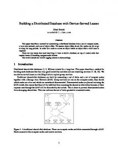
Building multiple representations is one of the key problems in GIS [Brugger et al. 89]. Indeed “hierarchical planning with different levels of detail for different parts of the task, seems to be common in human way-finding” [Mark 89]. However geographic databases are very similar to maps, i.e. only one representation at one scale is available. Nevertheless, a geographical database does not formally include the notion of scale (the ratio between the size of an object on the map and its real size on the ground) ; [Goodchild 91] [Müller et al. 95] speak of precision (degree of detail in the reporting of a measurement), accuracy (relationship between a measurement and the reality which it purports to represent) and resolution (the smallest object which can be represented). For geographic databases, it seems judicious therefore to connect the determination of these three concepts with the notion of scale commonly associated with a map. So, a multi-scale database is a geographic database, which allows us to represent the same phenomenon of the real world at different levels of precision, accuracy and resolution. Consequently, designing a multi-scale database requires a representation mechanism of schema and data at different levels. Three methods can be used to build a multi-scale database [Govorov 95] : • In the first method (see figure 1), a cartographic generalization1 process is used to generate databases at smaller scales from a single database at the greatest scale. Cartographic generalization can be either automatic or interactive. For the moment, this solution seems difficult for the following reasons :

1

Cartographic generalization modifies data in order to produce a simplified, or more abstracted representation, for the sake of map legibility [Lagrange and Ruas 94].

SDH’96

-1-

(i) There are no generalization tools in GIS allowing automatic generation representations less detailed than the most precise representation [Müller et al 95]. Indeed, modifications in cartographic generalization are complex, varied and intricately interwoven. (ii) An entirely interactive generalization is too long and too difficult [Müller 92] and for these reasons seems inadequate for final users. (iii) all the pieces of information which are wanted in the generalized representation, are not present in the most precise representation. Indeed, new themes may come on top of generalization. • The second method consists of a mere collection of geographic databases with no link whatsoever between objects. Some rules can be used to control the choice of the database to display according to the graphic scale. Nowadays, this method is implemented in some GIS (Apic, GeoConcept, ArcView) but these rules are limited (the notion of scale is unsuitable for geographical databases). For example, it would be necessary to include other parameters such as the density of the zone to define display rules. • Finally, in the third method (see figure 2), a multi-scale data structure is defined in order to link representations. This last solution seems the best compromise between the re-use of existing databases and their enrichment by integration. This is why we have adopted it. The aim of this integration is not to obtain a single representation but to allow interoperability between representations and to link homologous objects between the different representations of the same phenomenon of the real world. This integration is a “semantic integration” ; schemata are integrated according to the values of data. Input representations may be physically distributed databases or data sets. In the first case, we have one distributed database [Ceri and Pelagatti 87] or a federated database [Sheth and Larson 90], and in the second case we have a single database. This article discusses the latter type of multi-scale database.

Figure 1 : a single database with a cartographic generalization process

Figure 2 : multi-scale data structure Nevertheless, the design of multi-scale data structures is difficult, due to the implicit cartographic generalization complexity [Lagrange and Ruas 94]. We have therefore opted for the concept of scale-transition relationship [Devogele and Raynal 96] defined in section 2. We will then describe the process to build a multi-scale database in section 3. Note that this process has been experimented and validated on road network databases. Section 4 offers some conclusions.

2.

Designing a multi-scale database

In this section, we will first discuss some multi-scale database research given in the literature and its limitations. This will allow us to introduce the concept of the scale-transition relationship. Finally, the assets of the scale-transition relationship will be given.

2.1

Overview

Any geographic representation is an abstraction of the real world with its own concept to represent the phenomena of the real world. Designing a multi-scale database raises three kinds of problems: • Correspondence between abstractions. Abstraction translate phenomena of the real world into instances of databases, by focusing only on parts of these phenomena. From research on DBMS, only the concept of views [Günther 89] [Abel et al. 94] has been suggested to overcome this problem. However, scale problems are not approached in this context. • Correspondence between objects from different representations. Tree structures [Jones 91][Kidner and Jones 94][van Oosterom 95][Timpf and Frank 95] [Rigaux and Scholl 95] have been proposed to describe links between the different representations. However relationships in the real world are not always hierarchical when scale varies. • Defining the matching process between objects. Data matching is a generic term to indicate methods and algorithms to search two geographic sets of data for groups of objects that represent the same part of the SDH’96

-2-

real world. To identify homologous objects, geometric matchings [Raynal and Stricher 94] [Edwards 94] [Gabay and Doytsher 94] have been suggested. We will show that they are insufficient in our kernel. What is more, these three independent problems have never been coordinated.

2.2

Representations With Scale-Transition Relationships

To design multi-scale databases, it is necessary to integrate abstractions and to connect instances. With this aim, the concept of a scale-transition relationship which uses the object-oriented data model, is proposed. The concepts used in this article are those of type, class and object. • Type defines a template for all its objects. It provides a common representation for all objects of that type and a set of operations on those objects. A type can be an atomic type (integer, real, string, boolean and enumeration) or a structured type (tuple, set or list). Types are linked by subtyping (a type A is a subtype of another type B if an instance of A is a instance of B) and inheritance (a type A inherits from another type B if A shares all the behaviours of B). • Class is a grouping of instances of a given type. • Object is an instance of one type and is included in one class. Each object has both an invariant identifier (OID) and a value. With these concepts, we can define what a scale-transition relationship is. Scale-transition relationships connect two sets of elements (types, classes or objects) representing the same phenomenon of the real world and carry the sequence of multi-scale operations to go from one representation to another. Scale-transition relationships are oriented links. Since they include multi-scale operations, scale-transition relationships are describing and storing some amount of cartographic generalization. They are more advanced structures than simple relationships between elements. Multi-scale operations are defined in [Devogele and Raynal 95] and [Peng 96]. Two categories can be distinguished : • Cartographic generalization operations as described in [Shea and McMaster 91] and [McMaster and Shea 92]. • Schema modification operations which are basically borrowed from the database theory, and more precisely from schema evolution and schema integration such as those defined in [Motro 87] [Scherrer et al. 93] and [Scholl and Tresch 93]. For example, in figure 3, one can distinguish : -Scale-transition relationships between a set of buildings and a built-up area carrying the multi-scale operation : amalgamation [Shea and McMaster 91]. -Scale-transition relationships between a road section and another road section carrying the multi-scale operation : simplification [Shea and McMaster 91]. Of course, some elements may not match due to deletion in the less detailed representation.

amalgamation simplification Figure 3 : Representations with scale-transition relationships

2.3

Assets of scale-transition relationships

These scale-transition relationships can describe the correspondence between schemata (type and classe definitions) and to link data from different representations. Furthermore, a multi-scale database using scale-transition relationships allows us to answer the different needs of multi-scale database users : • From a practical point of view, this concept allows intelligent zoom [Timpf and Frank 95] between the different representations, and analysis of data from different representations. Queries can be applied SDH’96

-3-

simultaneously on sets of buildings and built-up areas even if these two classes are not defined in the same representation. Navigation between the different representations [Car and Frank 95] [Langou and Mainguenaud 94] is also feasible because scale-transition relationships authorize to go back and forth between representations. • Information transfers between levels also become possible, giving access to the sequence of multi-scale operations between elements. This means that, at least in some cases, it is possible to propagate an update performed at some detailed level, to a less detailed level [Kilpeläinen 95]. Indeed, once the scale-transition relationship carries enough information (precise sequence of multi-scale operations, values of parameters,…), the update, also required at the secondary level, may be activated through the conversion from the basic level. However, it is clear that such an automation might prove to be quite difficult if complex geometric transformations or transformations involving sets of objects are needed. • Finally for mapping agencies, the database merging favours quality control, and the concomitance of representations in a single structure facilitates maintenance of consistency. Besides, the information on quality (geometric accuracy, semantic accuracy, …) can be easily obtained by comparison of the less detailed database, to the reference database. In any case, building a multi-scale database allows us to derive new products and to integrate new data.

3.

Process to build a multi-scale database with scale-transition relationships

Two stages are distinguished in the process to build a multi-scale database : schema integration and data matching. • Schema integration allows interoperability between existing databases, since a multi-database language and an integrated data description can be defined. This first stage is inspired by works of [Spaccapietra et al. 92] [Dupont 94] that use assertion-based methodology. This methodology splits the integration process into two distinct steps. The first step is dedicated to the declaration of correspondences and conflicts between input schemata by using scale-transition relationships. In the second step, conflicts are resolved and schemata are merged. • In the second stage called data matching, homologous objects (representing the same real world phenomenon) are connected. This process generates scale-transition relationships between objects by using semantic, topologic and geometric information. Finally, to test the feasibility of such principles, a multi scale database kernel [Trevisan 95] has been realized from two IGN’s mono-scale databases (BD CARTO® 2 and GÉOROUTE® 3) in the area of Marne-la-Vallée (367 km of road for BD CARTO® and 991 km of road for GÉOROUTE®, the network in this area being varied and dense). This kernel has been developed in O2 [O2 91] and GéO2 [Raynal et al. 95] [David et al.93]. For the sake of easy reading the BDC acronym is adopted to designate BD CARTO® and the G acronym is adopted to designate GÉOROUTE®.

3.1

Declaration of Scale-Transition Relationships

Declaration of scale-transition relationships is done at two levels : between classes and between types.

BD CARTO® contains the basic geographical information, that is necessary for the production of 1:100,000 topographic maps, for national and regional development and network management. BD CARTO® has been created by processing existing 1:50,000 maps (scanning, vectorization, topological structuring). 2

GEOROUTE® is a topologically structured road-planning database containing precise data for urban areas and uses BD CARTO® data for other areas. GEOROUTE® is used for transportation purposes. 3

SDH’96

-4-

3.1.1 Scale-transition relationships between classes Scale-transition relationships between classes are used to describe correspondence between collections of instances ; i.e. they indicate that one instance of class 1 in the schema 1 corresponds to one instance of class 2 in the schema 2. More complex correspondences are also possible. For example, Crossroads classes do not correspond GÉOROUTE® BD CARTO® exactly : -One instance of the G Crossroads class corresponds to 0 or One instance of the BDC Crossroads class (whether it is suppressed or preserved). -One instance of the BDC Crossroads class can correspond to 1 complex crossroad in G (figure 4), which is composed of instances of Crossroads and Sections classes in G. Indeed, due to the change of scale, some instances of Sections and Crossroads classes are Figure 4 : The same crossroads in BDC and in G suppressed or are symbolised in a set of fewer objects. Extended to all classes in the kernel, the scale-transition relationships are : from BDC to G (Table 1) and from G to BDC (Table 2). BDC →G

G →BDC

1 Road

1 Road

1 Road

(0-1) Road

1 Section

(1-N) Sections

1 Section

(0-1) Section or 1 Crossroad

1 Crossroad

(0-N) Crossroads and (0-N) Sections

1 Crossroad

(0-1) Crossroad

Table 1 : Scale-transition relationships from BDC Table 2 : Scale-transition relationships from G classes to G classes classes to BDC classes Once scale-transition relationships between classes have been described, it is necessary to describe scale-transition relationships between types. 3.1.2 Scale-transition relationships between types Scale-transition relationships between types describe differences in structure. These scale-transition relationships can be declared only for types whose classes correspond. Scale-transition relationships between types can be declared according to the values of data in correspondence and not according to type parameters (name, domain,…). These differences are described by multi-scale operations (see section 2.2). For example, BDC crossroad type correspond to G crossroad type : they describe the same phenomenon of the real world. For tuples, attributes must be also link. These two tuples have three common attributes (kind_of_crossroad, and toponym, geometry). Furthermore the BDC type has one own semantic attribute: spot_height. - kind_of_crossroad attributes of BDC and G that describe the nature of the crossroad, are enumerations (authorized values : simple crossroads, roundabout, interchange, …). Globally, they correspond but some values have been added or suppressed. Thus, the multi-scale operation is a function of change for lists of authorized values. -Toponym attributes which indicate the name of the crossroad, correspond semantically but they do not have the same structure : in BDC, toponym is a tuple (attributes: Kind, Article, Wording) while in G, toponym is a character string. These, the multi-scale operation is a function of transformation of tuple into character string. -Geometry attributes correspond exactly, they represent points. There is no multi-scale operation associated with this scale-transition relationship. -Spot_height attribute is only present in BDC. So, the scale-transition relationship is a deletion. This example shows a few correspondences between types. The whole set of scale-transition relationships established in the prototype will be made available in [Trevisan 95].

3.2

Schema Merging

Schema Merging is the step that unifies corresponding types and corresponding classes to build the integrated schema. In this step, the best integration techniques are chosen for each kind of scale-transition relationship. The literature proposes several techniques to integrate schemata, depending on whether we prefer to preserve or to delete the initial schemata and on the kind of integrated schemata that we wish. In our case, we want to obtain SDH’96

-5-

a schema which will be able to represent all the instances of input schemata, without loss of information by unifying structures and will be able to connect data of different input representations most precisely. To transcribe scale-transition relationships between classes, the integration technique is to create a relationship between types corresponding to classes. For scale-transition relationships between one class and many classes (or between many classes and many classes), the integration technique is to create one (or many) super-class(es) and the relationship is carried by the types of these super-class(es) (see figure 5). Therefore, these super-types are anchor points to scale-transition relationships between instances. Thus for Crossroads and Sections of BDC and G, super-types Net_el_G (Network elements of G) and Net_el_BDC (Network elements of BDC) have been created and a relationship STR_Element (scale-transition relationship between network elements) has been defined between these two super-types. All scale-transition relationships between Sections and Crossroads classes (mentioned in tables 1 and 2) are grouped in these relationships. For scale-transition relationships between tuples, a technique of generalization between types has been chosen, i.e. for each pair of corresponding types (for example Crossroad types of BDC and G), a father type is created supporting common attributes (called Crossroad, in the kernel, see figure 5) and two son types are maintained for the specific attributes (called Crossroad_G and Crossroad_BDC, see figure 5). For scale-transition relationships between enumerated types (for example kind_of_crossroad of BDC and G) supporting functions of change for lists of authorized values as multi-scale operation, the chosen integration technique is to create a new enumerated type. This type is defined by merging authorized values of these two types. For scale-transition relationships between a tuple type and a primitive type (for example toponym types of BDC and G), the chosen integration technique depends on the complexity of the transformation mechanism. If the transformation process is manual, these types remain separated ; otherwise, the tuple type is preserved and the primitive type is transformed. The latter technique is applied for toponym types of BDC and G. Once this step is finished, we have a multi-scale schema allowing us to represent input types and to represent scale-transition relationships between their instances. This multi-scale schema can be either the schema of federated databases, or the schema of a single database with several data representations. Figure 5 presents the merged schema in our kernel. Road Id Num Adm_class administrator

is composed

Id Vocation Nb_ways Nb_total_lanes Nb_up_lanes Nb_down_lanes

Begin Node Section End Node Surface_state Access 2 {ordered} Position Communication Diversion_network Direction No_drive Geometry Weight_limit

Crossroad Id Toponym Kind_of_node Geometry

Hight_limit

Road_G

Road_BDC STR_Road Multi-scale_Ope

Section_G

Section_BDC Toponym Use Installation_day frost

Add_begin_left Standard_way Add_begin_right Width_limit Add_end_left Length_limit Add_end _right Vehicle_limit Specific_equipement

Father type Son type Relationship representing Scale-Transition Relationship

Crossroad_G

Crossroad_BDC spot_height

Net_El_G STR_Element Multi-scale_Ope Net_El_BDC

Figure 5 : Multi-scale schema (OMT model [Rumbaugh et al. 91]) This base supports two representations integrated in a single schema, but the objects themselves are not yet matched.

3.3

Data matching

Data matching is a generic term to indicate methods and algorithms to search two geographic sets of data for groups of objects that represent the same part of the real world. First, we will define the different types of data matching used, then we will describe the process realized in the kernel, before presenting some of the first results. 3.3.1 Different kinds of data matching In the current context (a single multi-scale database), the data matching step is realized after the schema merging. Scale-transition relationships between objects are therefore constructed in a permanent manner. To SDH’96

-6-

match data, semantic, topologic and geometric information is used to overcome the shortcomings of simple geometric matching as presented in [Raynal and Stricher 94] [Edwards 94] and [Gabay and Doytsher 94]. • The semantic matching put objects in correspondence according to their semantic attributes, which are a key. Objects are matched on the value of their keys. • The topologic matching uses composition or topologic relationships between the different objects to match data. If two relationships correspond, then this correspondence can be used to find homologous objects linked by this relationship. • The geometric matching ; data are matched by their location with a measure of distance between objects. Other geometrical characteristics, as the direction [Gabay and Doytsher 94] have been proposed to match these data. 3.3.2 Data matching process for the kernel These three kinds of matching have been necessary for the kernel. Furthermore, the process order is fundamental (data forming a network, many relationships exist between them). Thus three successive matching processes (see figure 6) have been defined : road matching, crossroad matching and section matching. Road_BDC Road Matching

( Road_G, Road_BDC )

Road_G

Sections Matching

Section_BDC

Crossroad_G

Road_BDC, Crossroad_BDC, Section_BDC

( Section_BDC, {Section_G} ) UNMATCHED DATA

Section_G

Crossroad_BDC

INCONCICTENCY

Crossroad Matching

Section_G

Road_G Crossroad_G Section_G

( Crossroad_BDC, {Crossroad_G, Section_G } )

Figure 6: Data matching process for the kernel Road matching : This algorithm uses only semantic information (keys are attributes : number and administrator) and generates object pairs (Road_BDC, Road_G). Crossroad matching : This procedure is more complex, using geometric and topologic information. Indeed, first, we automatically determine a search area4 Search around each BDC crossroad (see figure 7) ; G crossroads in area this area are automatically selected. Group 2 Then, by using topologic relationships between crossroad and section, we form connected groups (figure 5 : 4 connected groups). We compute the connected group whose dangle sections Group 3 Group 1 (sections connected to the group) and bi-connected sections (sections belonging to the group) match with dangle sections Group 4 of the BDC crossroad. On figure 5, we observe that group 1 matches with the BDC crossroad. This algorithm is used for all BDC crossroads and generates object pairs (Crossroad_BDC,{Crossroad_G,Section_G}. Figure 7: example of connected group Section matching : Henceforth, BDC sections may be matched with G sections (previously, G sections matched with BDC crossroads must be removed). This matching is achieved in two stages. In the first stage, sections belonging to semantically matched roads are matched road by road. Then the other sections are matched.

4

A search area is the intersection between a circle and the Voronoï diagram [Yap 87] of punctual BDC crossroads

SDH’96

-7-

Geometric section matching is realized with the help of the Hausdorff distance [Raynal and Stricher 94] [Hangouët 95] [Hausdorff 19]. We obtain three kinds of G sections : • Matched section : Only one distance of the BDC section from this G section is less than the matching threshold. • Litigious section : Several distances of the BDC section are less than the matching threshold. We can not choose the homologous BDC section with distance alone. • Unmatched section : No distance of BDC section is less than the matching threshold. Either this section has no homologue, or this section has one homologue but distance is superior to the matching threshold. Although those last two matching algorithms are not optimal (certainly, one can integrate more semantic information), a process which has been able to match real data sets has been realized [Trevisan 95]. We can present the first results. 3.3.3 First results Results of road matching are 100% correct. As for crossroads, a manual match was also performed to check the automatic process. For 284 crossroads, results are as follows : • For one BDC to one G matching (191 cases), automatic matching gives good results in 84% of cases. The remaining 16% are results including the right result but also some parasitic elements. • For one BDC to many G (49 cases) results are average. Automatic matching gives good results in 41% of cases, gives a result containing only a part of the right result in 28.5%, and gives a result including the right result in 30.5%. No matching between BDC crossroads and G crossroads (44 cases), has been also analyzed: • The main reason is border objects (49.4%) for which some dangle sections are missing (in BDC or in G). • The second reason of mismatch is inconsistency (39%) ; updates are not the same and semantic or geometric quality is wrong. • The third set of reasons are conflicts between BDC crossroads being too close (5.8%): a part of the complex crossroad can not be matched with the BDC crossroad because it is in another research area [Trevisan 95]. • The last set of causes are the translations (5.8%) between the two representations that are superior to the matching threshold. Results of section matching are approximately 75% correct.

3.4 Generalization of this process Our building a multi-scale database for road network data has demonstrated the feasibility of such databases from data sets. This process can be generalized whatever : • the data (network, land use, topography, …). For example, for land use data, the schema integration phase does not change much, on the other hand the data matching phase necessitates a new process [Kidner 96] (distance between surfaces, relationship of neighbourhood, …). • the number of representations. This process can be generalized to more than two input databases by using the same methods (schema integration into a single schema then, matching two by two of instances). • the location of representations (data set, distributed databases). For the integration of distributed databases into a federated database, our first results will still have to be improved. Indeed, with autonomous databases, data matching will not be computed after schema merging, but during the processing of the multi-scale queries and only for the data involved. This “on the fly” process is very interesting but necessitates a very effective matching process. • the needs (data analysis, quality controls, …). According to the application chosen, the multi-scale schema will not comply with the same constraints. Therefore, the schema integration technique is different. Building multi-scale database is an adaptable process. This process depends on the data, the needs, the number and the location of representations. This work can be also generalized for different kinds of multiple representations (temporal, thematic,…). In this cases, new operations of correspondence will have to be defined.

4.

Conclusion

In this article, we have described a process to build a multi-scale database with scale-transition relationships. This is a three steps process : declaration of scale-transition relationships between schemata, schema merging and data matching. Because management of this kind of database is difficult, some problems must be first tackled (update, data manipulation language,…). This process must still be thorough, by optimizing the data matching and by working on the retrieve-and-store of multi-scale operations. We are continuing our research SDH’96

-8-

into the integration of geographic databases (databases from different sources or databases stemming from a generalization process).

References D.J. Abel, P.J. Kilby and J. R. Davis (1994) The systems integration problem, in Int. J. Geographical Informations Systems Vol. 8 N° 1, pp 1-12. B. P. Brugger, R. Barrera A. U. Frank, K. Beard and M. Ehlers (1989) Research Topic on Multiple Representations in NCGIA Initiative 3 Workshop on Multiple Representations, pages 53-67. A. Car, A.U. Frank (1994), Modelling a Hierarchy of Space applied to Large Road Networks, in IGIS’94, LNCS n°884, pp 15-24. S. Ceri et G. Pelagatti (1987) Distributed databases: principles & systems, McGraw-Hill. B. David, L. Raynal, G. Schorter and V. Mansart (1993) Why objects in a geographical DBMS?, in Advances in Spatial Databases, pp 264-276. T. Devogele, L. Raynal. (1996) Modeling a Multi-Scale Database with Scale-Transition Relationships, in Samos’96, T.Sellis D. Georgoulis Eds. pp 83-93 Y. Dupont (1994) Resolving Fragmentation Conflicts in Schema Integration in 13th Int. Conf. on The Entity Relationship Approach. G. Edwards (1994) Characterising and maintaining polygons with fuzzy boundaries in geographic information systems, in Spatial Data Handling,Waugh and Healey Eds., Taylor&Francis, pp 223-239 Y. Gabay and Y. Doytsher (1994) Automatic adjustement of line maps, in GIS/LIS pp 233-241. M.F. Goodchild (1991) Issue of quality and uncertainty, in Advances in Cartography, Müller Ed., Barking, Essex/ Elsevier pp 113-139. M.O. Govorov (1995) Representation of the generalized data structures for Multi-Scale GIS, in 17 th ICA/ACI Barcelonna pp 2491-2495. O. Günther (1989) Database Support for Multiple Representations, NCGIA, in Initiative 3 Workshop on Multiple Representations, pp 50-51 C.B. Jones (1991) Database architecture for multi-scale GIS, in Auto-Carto 10 volume 6 pp 1-14. J.F. Hangouët (1995) Computation of the Hausdorff distance between plane vector polylines, in Auto Carto 12, pp 1-10. F. Hausdorff (1919) Dimension und äusseres in Mass. Mathematische Annalen n° 79, pp 157-179. D. Kidner and C.B. Jones (1994) A Deductive Object-Oriented GIS for handling multiple representations, in Spatial Data Handling, Waugh and Healey Eds., Taylor&Francis, pp 882-900. D. Kidner (1996) Geometric signatures for determing polygon equivalence during multi-scale GIS update, in Second Joint European Conference, IOS Press, pp 239-247. J.P. Lagrange and A. Ruas (1994) Geographic information modelling: GIS and generalisation, in Spatial Data Handling, Waugh and Healey Eds., Taylor&Francis, pp 1099-1117. B. Langou and Maiguenaud M. (1994) Graph data model operations for network facilities in a geographical information system, in Spatial Data Handling, Taylor & Francis, pp 1002-1019. T. Kilpeläinen (1995) Requirements of a Multiple representation database for topolographical data with emphasis on incremental generalization, in 17 th ICA/ACI Barcelonna, pp 1815-1825. D. Mark (1989) Multiple views of multiple representations, in NCGIA Initiative 3 Workshop on Multiple Representations, pp 68-71. R. McMaster and S. Shea (1992), Generalization in Digital Cartography, Association of American Geographers. A. Motro (1987) Superviews; Virtual Integration of Multiple Databases, in IEEE Transactions on Software Engineering 13 (7), IEEE, pp 785-798. J.C. Müller (1991) Generalization of spatial databases, Geographical information Systems Principles and Applications, Maguire, Goodchild and Rhind Eds., Publisher Longman Scientific & Technical, pp 457-475 J.C. Müller, J.P. Lagrange, R. Weibel and F. Salgé (1995) Generalisation : state of the art and issues, in GIS and GENERALISATION, Müller, Lagrange and Weibel Eds., Taylor & Francis pp 3-17. O2 (1991) The O2 System; in Communications of the ACM, Vol 34,n°10. W. Peng, K. Tempfi and M. Molenaar (1996) Automated Generalization in a GIS, Geoinformatic’96, West Palm Beach pp 135-146

SDH’96

-9-

L. Raynal, B. David and G. Schorter (1995) Building an OOGIS prototype: experiments with GeO2, in Auto Carto 12 pp 137-146. L. Raynal and N. Stricher (1994) Base de données multi-échelles: Association géométrique des tronçons de route de la BD Carto et de la BD Topo in EGIS /MARI’94, pp 300-307. P. Rigaux and M. Scholl (1995) Multi-Scale Partitions: Application to Spatial and Statistical Databases in SSD ‘95, pp 170-183. J. Rumbaugh, M. Blaha, W. Premerlani, F. Eddy and W.Lorensen (1991) Object-Oriented modeling and design, Prentice Hall Eds., Englewood Cliffs. S. Scherrer,A. Geppert and K. Dittrich (1993) Schema Evolution in NO 2, Institut fur Informatik der Universitat Zurich technical report n° 93-12. M.H. Scholl and M. Tresch. (1993) Schema Transformation without database reorganisation, in ACM SIGMOD Record, (22;1). K.S. Shea and R.B. McMaster (1991) Cartographic Generalisation in a digital environment When and how to generalize, in Map generalization, Buttenfield and McMaster Eds., Longman Scientific & Technical, pp 103-118. A. Sheth et J. Larson (1990) Federated database systems for managing distributed, heterogeneous, and autonomous databases,in ACM Computer Surveys 22,3 (Sept 1990), pp 183-236 S. Spaccapietra, P. Parent, Y. Dupont, (1992) Model-Independent Assertions for Integration of Heterogeneous Schemas, in Very Large DataBases Journal, 1(1), pp 81-126. S. Timpf and U. Frank (1995) A Multi-scale DAG for cartographic objects, in Auto Carto 12, pp 157-163. J. Trevisan (1995) Conception d’une BD Multi-échelles, ENSG Academic report, IGN Saint Mandé. P. van Oosterom (1995) The GAP-tree, an approach to 'on-the-fly' map generalisation of an area partitioning, in GIS and GENERALISATION, Müller, Lagrange and Weibel Eds., Taylor & Francis, pp 120-132. C.K. Yap (1987) An O(n log n) Algorithm for the Voronoï Diagram of a set of simple Curve Segments in Discete Comp. Geom. 2 journal, pages 365-393.

SDH’96

- 10 -