Building Simulation Models with Simscript II.5

process AIRPLANE call TOWER giving GATE yielding RUNWAY work TAXI.TIME (GATE, RUNWAY) minutes request 1 RUNWAY work TAKEOFF.TIME (AIRPLANE) minutes relinquish 1 RUNWAY end " process AIRPLANE process AIRPLANE call TOWER giving GATE yielding RUNWAY work TAXI.TIME (GATE, RUNWAY) minutes request 1 RUNWAY

S

Since

1962

Building Simulation Models with Simscript II.5 Edward C. Russell

Building Simulation Models with SIMSCRIPT II.5 Edward C. Russell

Copyright  1999 CACI Products Co. February 1999 All rights reserved. No part of this publication may be reproduced by any means without written permission from CACI. For product information or technical support contact:

CACI Products Company 3333 North Torrey Pines Court La Jolla, California 92037 Phone: (619) 824.5200 Fax: (619) 457.1184

The information in this publication is believed to be accurate in all respects. However, CACI cannot assume the responsibility for any consequences resulting from the use thereof. The information contained herein is subject to change. Revisions to this publication or new editions of it may be issued to incorporate such change. SIMGRAPHICS I, SIMGRAPHICS II and SIMSCRIPT II.5 are registered trademarks of CACI Products Company.

Windows is a registered trademark of Microsoft Corporation.

Table of Contents 1. Preface ............................................................................................................ a 1.1 FREE T RIAL OFFER ................................................................................................................ b 1.2 TRAINING COURSES ............................................................................................................... b 1.3 WEB S ITE .............................................................................................................................. b

1. Introduction .................................................................................................... 1 1.1 WHAT IS SIMULATION ? ......................................................................................................... 1 1.2 WHAT IS WRONG WITH S IMULATION? ................................................................................... 3 1.3 HOW TO A VOID THE TEN BIG MISTAKES ................................................................................ 3 1.3.1 Failure to Define an Achievable Goal ......................................................................... 3 1.3.2 Incomplete Mix of Essential Skills ............................................................................... 4 1.3.3 Inadequate Level of User Participation ....................................................................... 4 1.3.4 Inappropriate Level of Detail ....................................................................................... 4 1.3.5 Poor Communication .................................................................................................. 5 1.3.6 Using the Wrong Computer Language ....................................................................... 5 1.3.7 Obsolete or Nonexistent Documentation .................................................................... 5 1.3.8 Using an Unverified Model .......................................................................................... 6 1.3.9 Failure to Use Modern Tools and Techniques to Manage the Development .............. 6 1.3.10 Using Mysterious Results ......................................................................................... 7 1.4 A FIRST LOOK AT THE SIMULATION TASK .............................................................................. 7 1.4.1 1.4.2 1.4.3 1.4.4 1.4.5 1.4.6 1.4.7 1.4.8

Articulate Simulation Goals ......................................................................................... 7 Analyze the System to Determine the Appropriate Level of Detail for the Model ....... 8 Synthesize the System (Realize the Model) ............................................................... 8 Collect and Prepare Input Data ................................................................................... 8 Verify the Model .......................................................................................................... 8 Validate the Model ...................................................................................................... 9 Conduct Experiments .................................................................................................. 9 Analyze the Results .................................................................................................... 9

1.5 MANUAL CONTENTS ............................................................................................................. 9

2. Elementary Modeling Concepts ................................................................. 11 2.1 2.2 2.3 2.4

MODEL STRUCTURE ........................................................................................................... 11 PROCESS CONCEPT ........................................................................................................... 12 RESOURCE CONCEPT ......................................................................................................... 12 PROGRAM STRUCTURE ....................................................................................................... 13

2.4.1 2.4.2 2.4.3 2.4.4

Preamble ................................................................................................................... 13 Main .......................................................................................................................... 13 The Timing Routine ................................................................................................... 14 Process Routines ...................................................................................................... 15

2.5 EXAMPLE 1: A S IMPLE GAS STATION ................................................................................. 15 2.6 ADDING P ERFORMANCE MEASUREMENTS ............................................................................ 19 2.7 A SLIGHTLY MORE COMPLICATED EXAMPLE ........................................................................ 22 2.7.1 2.7.2 2.7.3 2.7.4

Define to Mean .......................................................................................................... 22 Local Variables ......................................................................................................... 25 Simple Decision Logic ............................................................................................... 25 Concluding Remarks ................................................................................................. 25

3. Modeling Individual Objects ....................................................................... 27 3.1 ATTRIBUTE CONCEPT ......................................................................................................... 27

i

Building Simulation Models with SIMSCRIPT II.5

3.2 VARIABLES ......................................................................................................................... 28 3.2.1 Global/Local Conflicts ............................................................................................... 28 3.2.2 Naming of Variables .................................................................................................. 29 3.3 ARITHMETIC ....................................................................................................................... 29 3.4 DATA INPUT ....................................................................................................................... 30 3.5 PROGRAM CONTROL S TRUCTURES ..................................................................................... 31 3.5.1 IF Statement ............................................................................................................. 31 3.5.2 Looping ..................................................................................................................... 32 3.6 REPRESENTATION OF TIME ................................................................................................. 34 3.7 TIME MEASUREMENTS ........................................................................................................ 34 3.8 EXAMPLE 3: A B ANK WITH A S EPARATE QUEUE FOR EACH T ELLER .................................... 35 3.8.1 Model Formulation .................................................................................................... 35 3.8.2 Program Discussion ................................................................................................... 39 3.9 PROCESS A TTRIBUTES ....................................................................................................... 40 3.10 ARGUMENT PASSING FOR S UBROUTINES ........................................................................... 42 3.11 SUBPROGRAM VARIABLES ................................................................................................ 43 3.12 ARGUMENT PASSING FOR P ROCESSES .............................................................................. 44 3.13 PROCESS INTERACTION COMMANDS ................................................................................. 45 3.13.1 Suspend .................................................................................................................. 47 3.13.2 Destroy .................................................................................................................... 47 3.14 SET CONCEPT .................................................................................................................. 48 3.15 EXAMPLE 4: A HARBOR MODEL ....................................................................................... 51 3.15.1 Model Formulation .................................................................................................. 51 3.15.2 Program Discussion ................................................................................................ 55 3.16 SUMMARY ........................................................................................................................ 56

4. Modeling and Measuring Random Phenomena .......................................57 4.1 INTRODUCTION ................................................................................................................... 57 4.2 RANDOM NUMBER GENERATION ......................................................................................... 57 4.3 RANDOM DEVIATES ............................................................................................................ 58 4.3.1 Uniform ..................................................................................................................... 59 4.3.2 Normal ...................................................................................................................... 59 4.3.3 Exponential ............................................................................................................... 60 4.3.4 GAMMA .................................................................................................................... 61 4.3.5 Beta........................................................................................................................... 62 4.3.6 Erlang ........................................................................................................................ 63 4.3.7 Log Normal ............................................................................................................... 64 4.3.8 Weibull ...................................................................................................................... 65 4.3.9 Integer Uniform ......................................................................................................... 65 4.3.10 Poisson ................................................................................................................... 66 4.3.11 Binomial .................................................................................................................. 67 4.4 4.5 4.6 4.7

ARBITRARY RANDOM V ARIABLES ......................................................................................... 67 CONTROLLING P ERFORMANCE MEASUREMENTS ................................................................... 70 ADDITIONAL S TATISTICAL PERFORMANCE MEASURES ........................................................... 72 E XAMPLE 5: THE “MODERN” B ANK (SINGLE -QUEUE -MULTIPLE -S ERVER ) .............................. 74

4.7.1 Model Formulation .................................................................................................... 74 4.7.2 Program Discussion .................................................................................................. 77

ii

Contents

4.8 DISCUSSION

OF

RESULTS ................................................................................................... 79

5. Modeling Passive Objects .......................................................................... 81 5.1 5.2 5.3 5.4 5.5 5.6

INTRODUCTION ................................................................................................................... 81 PERMANENT E NTITIES ........................................................................................................ 81 COMPOUND E NTITIES ......................................................................................................... 82 TEMPORARY E NTITIES ........................................................................................................ 83 A SECOND L OOK AT S ETS ................................................................................................. 86 ADDITIONAL SET MANIPULATIONS ....................................................................................... 89

5.6.1 5.6.2 5.6.3 5.6.4 5.6.5

IN Reverse Order ...................................................................................................... 89 FILE FIRST and FILE LAST ..................................................................................... 89 REMOVE FIRST and REMOVE LAST ..................................................................... 89 REMOVE Entity ........................................................................................................ 89 FILE BEFORE and FILE AFTER .............................................................................. 90

5.7 EXAMPLE 6: A JOB S HOP MODEL ....................................................................................... 90 5.7.1 Model Formulation .................................................................................................... 90 5.7.2 Program Discussion .................................................................................................. 97 5.8 MORE EFFICIENT USE OF DATA STORAGE .......................................................................... 98 5.9 EFFICIENCY IMPROVEMENTS FOR SET S TRUCTURES .......................................................... 101 5.10 SYSTEM A TTRIBUTES AND A RRAYS .................................................................................. 102

6. Miscellaneous Simulation Topics ............................................................ 107 6.1 INTRODUCTION ................................................................................................................. 107 6.2 EXTERNAL P ROCESSES .................................................................................................... 107 6.2.1 Process Name ........................................................................................................ 108 6.2.2 Process Activation Time ......................................................................................... 108 6.3 PRIORITY AND TIE-BREAKING AMONG P ROCESSES ............................................................ 112 6.4 PRIORITY QUEUEING FOR RESOURCES ............................................................................. 115 6.5 EXAMPLE 7: A COMPUTER CENTER S TUDY ...................................................................... 117 6.5.1 Model Formulation .................................................................................................. 118 6.6 MONITORED A CTIONS ....................................................................................................... 121 6.7 MONITORED V ARIABLES .................................................................................................... 123 6.7.1 Program Discussion ................................................................................................ 124

7. Modeling With Discrete Events ................................................................ 129 7.1 7.2 7.3 7.4

INTRODUCTION ................................................................................................................. 129 ANALOGY B ETWEEN PROCESSES AND EVENTS .................................................................. 129 EXAMPLE 8: GAS S TATION 1A REVISITED ......................................................................... 130 ADDITIONAL EVENT COMMANDS ........................................................................................ 133

7.4.1 Cancel Statement ................................................................................................... 133

8. Input and Output ........................................................................................ 135 8.1 INTRODUCTION ................................................................................................................. 135 8.2 REVIEW : F REE -F ORM READ AND THE PRINT S TATEMENT .................................................. 135 8.3 TEXT MODE .................................................................................................................... 137 8.3.1 8.3.2 8.3.3 8.3.4

Free-Form Input ...................................................................................................... 137 CONCAT.F(A, B) .................................................................................................... 138 LENGTH.F (A) ........................................................................................................ 138 MATCH.F (A, B, I) ................................................................................................... 138 iii


8.3.5 8.3.6 8.3.7 8.3.8 8.3.9

SUBSTR.F (A, I, J) .................................................................................................. 139 TTOA.F(A) .............................................................................................................. 139 ITOT.F(I) ................................................................................................................. 139 Text Comparisons ................................................................................................... 139 Storage Considerations .......................................................................................... 140

8.4 REPORT GENERATOR ....................................................................................................... 140 8.4.1 Automatic Page Titling ............................................................................................ 140 8.4.2 System Variables Related to Output ....................................................................... 141 8.4.3 Multiple Page-Width Reports (Column Repetition) ................................................. 143 8.5 FORMATTED INPUT /OUTPUT ............................................................................................... 145 8.5.1 8.5.2 8.5.3 8.5.4

Example 1 ............................................................................................................... 150 Example 2 ............................................................................................................... 150 Example 3 ............................................................................................................... 151 Repeating a Format ................................................................................................ 151

8.6 MULTIPLE INPUT /OUTPUT DEVICES ................................................................................... 151 8.7 MISCELLANEOUS INPUT /OUTPUT FEATURES ...................................................................... 153 8.7.1 8.7.2 8.7.3 8.7.4 8.7.5

Rewind Statement ................................................................................................... 153 Using Phrase .......................................................................................................... 154 Buffer ...................................................................................................................... 154 Input/Output of Binary Information .......................................................................... 155 External Process or Event ...................................................................................... 155

9. Model Verification and Debugging .......................................................... 157 9.1 9.2 9.3 9.4

INTRODUCTION ................................................................................................................. 157 COMPILER AIDS IN DEBUGGING ........................................................................................ 157 RESOLVING LINKER NAME CONFLICTS .............................................................................. 162 RUN -TIME DEBUGGING A IDS ............................................................................................. 163

9.4.1 Error Message ........................................................................................................ 164 9.4.2 Traceback ............................................................................................................... 164 9.4.3 System Conditions .................................................................................................. 164 9.5 EXAMPLE 9: THE HARBOR MODEL REVISITED ..................................................................... 164 9.6 USER -WRITTEN DEBUGGING ROUTINES ............................................................................. 172 9.6.1 SNAP.R — User Supplied Post Mortem Routine .................................................... 172 9.6.2 BETWEEN.V — Tracing the Flow of Simulation ..................................................... 173

10. A Comprehensive Example .................................................................... 185 10.1 10.2 10.3 10.4

INTRODUCTION ................................................................................................................ 185 THE P ROBLEM: A WATERWAYS NETW ORK ....................................................................... 185 INTRODUCTION TO THE SOFTW ARE DESIGN DOCUMENTATION L ANGUAGE (SDDL) ............. 185 MODEL DESIGN ............................................................................................................... 188

References ...................................................................................................... 201 Appendix A: SIMSCRIPT Reference Syntax ................................................ 203 A.1 A.2 A.3 A.4 A.5

iv

BASIC CONSTRUCTS .......................................................................................................... 203 PRIMITIVES ....................................................................................................................... 204 METAVARIABLES ............................................................................................................... 204 THE S TATEMENT SYNTAX .................................................................................................. 208 PREAMBLE STATEMENT PRECEDENCE RULES .................................................................... 224

Contents

Appendix B. SIMSCRIPT II.5 Coding Conventions ..................................... 227 B.1 CODE INDENTATION CONVENTIONS .................................................................................... 228 B.2 STRUCTURED PROGRAMMING ............................................................................................ 230 B.3 IMPLIED S UBSCRIPTS ........................................................................................................ 230

Appendix C. SIMSCRIPT II.5 Random Deviate Generator .......................... 231 C.1 Routine Listings ............................................................................................................. 231 C.2 INITIAL RANDOM NUMBER S TREAM S EEDS - SEED.V ....................................................... 231

Appendix D. System-Defined Names .......................................................... 239 D.1 D.2 D.3 D.4 D.5 D.6 D.7

VARIABLES ....................................................................................................................... 239 CONSTANTS ..................................................................................................................... 248 SYSTEM-DEFINED A TTRIBUTES .......................................................................................... 249 SYSTEM GENERATED NAMES ............................................................................................ 254 ATTRIBUTES GENERATED IN CONJUNCTION WITH USER -DEFINED ENTITIES ......................... 255 FUNCTIONS ...................................................................................................................... 259 ROUTINES ........................................................................................................................ 280

Index ................................................................................................................. 283

v


vi

List of Figures Figure 2-1. Basic SIMSCRIPT II.5 Timing Routine ..................................................................... 14 Figure 2-2. Time-Dependent Statistics........................................................................................ 20 Figure 3-1. Pump Resource Data Structure ................................................................................ 27 Figure 3-2. Input Data Mode Conversions .................................................................................. 31 Figure 3-3. Time-Independent Statistics ..................................................................................... 35 Figure 3-4. Multiple Process Data Structures ............................................................................. 41 Figure 3-5. Actions Performed for a Process (External to the Process, Itself) ............................ 45 Figure 3-6. Actions a Process Performs for Itself ........................................................................ 46 Figure 3-7. Set Structure Linkage ............................................................................................... 48 Figure 4-1. Uniform Distribution .................................................................................................. 59 Figure 4-2. Normal Distribution ................................................................................................... 60 Figure 4-3. Exponential Distribution ............................................................................................ 60 Figure 4-4. Gamma Distribution .................................................................................................. 62 Figure 4-5. Beta Distribution ....................................................................................................... 63 Figure 4-6. Erlang Distribution .................................................................................................... 64 Figure 4-7. Log Normal Distribution ............................................................................................ 64 Figure 4-8. Weibull Distribution ................................................................................................... 65 Figure 4-9. Integer Uniform Distribution ...................................................................................... 66 Figure 4-10. Poisson Distribution ................................................................................................ 66 Figure 4-11. Binomial Distribution ............................................................................................... 67 Figure 4-12. Example of Discrete Valued Random Variable........................................................ 68 Figure 4-13. Example of Continuous Random Variable .............................................................. 69 Figure 4-14. RESET Example ..................................................................................................... 71 Figure 5-1. Permanent Entity Data Structure .............................................................................. 82 Figure 5-2. Temporary Entity Data Structure .............................................................................. 84 Figure 5-3. Multiple Instances of a Temporary Entity .................................................................. 85 Figure 5-4. Linked Entities .......................................................................................................... 85 Figure 5-5. A Unidirectional Network .......................................................................................... 87 Figure 5-6. Network Structure ..................................................................................................... 87 Figure 5-7. Packed Temporary Entity ......................................................................................... 99 Figure 5-8. Packed Permanent Entity ....................................................................................... 100 Figure 5-9. Intra-Packing Permanent Entity .............................................................................. 101 Figure 5-10. Intra-Packing System Attribute ............................................................................. 104 Figure 5-11. Ragged Array Storage Allocation ......................................................................... 105 Figure 6-1. Event Set ................................................................................................................ 113 Figure 6-2. Detailed Resource Mechanism ............................................................................... 116 Figure 6-3. Before and After Arguments ................................................................................ 122 Figure 6-4. Example of Monitored Variables ............................................................................. 124 Figure 6-5. Inventory Measurements Using Monitored Variables ............................................. 126 Figure 8-1. Column Repetition Illustration ................................................................................. 143 Figure 8-2. Column Repetition Continuation Page .................................................................... 144 Figure 8-3. Illustration of Column Suppression ......................................................................... 145 Figure 9-1. A Routine from Example 4 (With Compilation Errors) ............................................. 158 Figure 9-2. The STAR Listing of Example 4 (Extract) .............................................................. 160 Figure 9-3. The ALLSTARS Listing of Example 4 (Extract) ................................................... 161 Figure C.1 SIMSCRIPT II.5 Random Deviate Generator Routine Listings ............................... 232

vii


viii

List of Examples Example 1. A Simple Gas Station Model ........................................................... 16 Detailed Trace of Execution ................................................................................................ 18 With Performance Measurements Added ........................................................................... 21 Output ................................................................................................................................. 22

Example 2. A More Elaborate Gas Station Model .............................................. 23 Output ................................................................................................................................. 24

Example 3. A Bank With a Separate Queue for Each Teller ..............................37 Output ................................................................................................................................. 38

Example 4. A Harbor Model ............................................................................... 51 Output ................................................................................................................................. 54

Example 5. The Modern Bank (Single-Queue-Multiple-Server) ......................... 75 Output ................................................................................................................................. 78

Example 6. A Job Shop Model ........................................................................... 91 Input ................................................................................................................................... 95 Output ................................................................................................................................ 96

Example 7. A Computer Center Study ............................................................. 118 Input ................................................................................................................................. 121 Output .............................................................................................................................. 121

Example 8. Gas Station Example 1A Revisited ................................................ 131 Output .............................................................................................................................. 132

Example 9. Harbor Model with Errors ............................................................... 165 Standard SIMSCRIPT Error Information .......................................................................... 170 With Diagnostic Programming Added .............................................................................. 175 User-Generated Diagnostic Output .................................................................................. 183

Example 10. Waterways Network Model .......................................................... 189

ix


x

Preface This document describes how to build simulation models using the CACI Product Company’s SIMSCRIPT II.5 programming system. SIMSCRIPT II.5 is an integrated, interactive development environment controlled by SimLab. SimLab includes the complete SIMSCRIPT II.5 programming language, utilities for editing and managing SIMSCRIPT II.5 programs, the SIMGRAPHICS I and II graphical interface and utilities, and comprehensive online-help. This document is an updated version of the book written by Edward C. Russell. It stresses the use of SIMSCRIPT II.5 for conceptualizing models and implementing them in computer-readable form. It presents the use of SIMSCRIPT II.5 for discrete-event simulation through a sequence of case studies. These range from a very simple model of a single-queue-single-server to a complete, complex network model. The examples have been throughly tested and used in a short course regularly offered by CACI. Although the examples illustrate all the features of SIMSCRIPT II.5, the emphasis is on model building. Consequently, programming concepts are introduced only as they are required. Appendix A describes the syntax of the entire SIMSCRIPT II.5 language in convenient form. This manual is oriented toward real applications. Small examples are used for practical reasons, but the techniques apply to large models as well. The intent is to stress good techniques of model building, program planning, programming, and verification. For information on how to build Graphical User Interfaces (GUI) and how to add animation and presentation graphics to simulation models, refer to the SIMGRAPHICS User’s Manual for SIMSCRIPT II.5. The following documents also pertain to SIMSCRIPT II.5: •

SIMSCRIPT II.5 Programming Language — A description of the programming techniques used in SIMSCRIPT II.5.

•

SIMSCRIPT II.5 Reference Handbook — A complete description of the SIMSCRIPT II.5 programming language.

•

SIMGRAPHICS II User’s Manual for SIMSCRIPT II.5 — Information about SIMGRAPHICS II, the integrated graphics development and animation environment for SIMSCRIPT II.5.

•

SIMGRAPHICS I User’s Guide and Casebook — Supplementary information on SIMGRAPHICS, and user’s guide for SIMGRPAHICS I.

•

SIMSCRIPT II.5 Windows User’s Manual — An instruction manual for Windows and Windows NT users of SIMSCRIPT II.5.

•

SIMSCRIPT II.5 UNIX User’s Manual — An instruction manual for UNIX users of SIMSCRIPT II.5.

a


The SIMSCRIPT II.5 language and its implementations are proprietary program products of the CACI Products Company. Distribution, maintenance, and documentation of the SIMSCRIPT II.5 language and compilers are available exclusively from CACI.

Free Trial Offer SIMSCRIPT II.5 is available on a free trial basis. We provide everything needed for a complete evaluation on your computer. There is no risk to you.

Training Courses Training courses in SIMSCRIPT II.5 are scheduled on a recurring basis in the following locations: La Jolla, California Washington, D.C. London, United Kingdom On-site instruction is available. Contact CACI for details. For information on free trials or training, please contact the following: CACI Products Company 3333 N. Torrey Pines Court La Jolla, CA 92037 (619) 824.5200 Fax: (619) 457.1184

Web Site For the most up-to-date SIMSCRIPT II.5 information, visit our WEB site at: www.caciasl.com

b

1. Introduction This chapter defines discrete-event simulation, broadly outlines the steps taken in simulation and model building, defines some common tools used in building simulation models and analyzes why simulations sometimes fail.

1.1 What is Simulation? Simulation is an effective way to pretest proposed systems, plans, or policies before developing expensive prototypes, field tests, or actual implementations. Using computerbased simulation, it is possible to trace out in detail the consequences and implications of a proposed course of action. Simulation can be defined as: •

The operation of a model that is a representation of the system under study.

•

Being amenable to manipulation that would be impossible, too expensive, or too impractical to perform on the system it portrays. Operation of the model being amenable to study. From the study, properties concerning the behavior of the actual system can be inferred.

•

This definition is broad enough to encompass methods other than the SIMSCRIPT II.5 approach discussed in this manual, but it will serve as a working definition that will be refined later. Simulation is often used as an alternative to more traditional forms of analysis such as analytical solutions (e.g. closed-form solutions to steady-state queueing models), numerical solutions (e.g., to differential equations), or even to scale-model building (e.g. for harbors or waterway systems). Over the past 20 years, simulation has proved again and again that it can be a powerful analytic tool. In small-scale applications, it has recorded countless modest successes; in large-scale applications, it has recorded some spectacular, widely publicized successes. The wonder is that a tool of such power has not gained even wider adoption. In her article Simulation as an Alternative to Linear Programming [17], Professor Susan L. Solomon comments wryly on the lingering distrust of simulation even as its use is becoming more widespread than ever: It is commonly accepted that general classes of problems are best solved using particular techniques. For example, critical path scheduling problems can often be formulated for solution by linear programming, but this approach would not recommend itself for cost reasons to the vast majority of those having access to a PERT or CPM package . . . Simulation might offer a reasonable alternative solution vehicle in many circumstances like

1


these, yet some operations research analysts tend to consider its use only “when all else fails.” That is, simulation is the technique of last resort. An examination of the simulation literature, including conference proceedings, in the past decade—by weight, by volume, by complexity and sophistication, or by breadth of application areas—would incline one to believe that either all else fails quite a bit of the time, or perhaps that simulation is a cost-effective alternative to the more structured deterministic methods of problem solving. Perhaps some analysts regard simulation as too difficult or merely too strange, and feel themselves on safer ground solving familiar, purely mathematical models. More likely, they are scared off by some of simulation’s spectacular—and costly failures. In paragraph 1.2 ten reasons are given for why simulations fail. The rest of this manual tells you how to succeed. Within the discipline of computer-based simulation, there is a rather clear-cut dichotomy between so-called “continuous simulation” and “discrete-event simulation.” Continuous simulation describes systems by sets of equations to be solved numerically. These may be algebraic or differential equations, usually with time as the independent variable. Examples of problems in this area are fluid-flow and hydraulics problems, heat-flow problems such as the representation of a blast furnace in a steel mill, and orbital calculations for a communications satellite. Discrete-event simulation describes a system in terms of logical relationships that cause changes of state at discrete points in time rather than continuously over time. Examples of problems in this area are most queueing situations: Objects (customers in a gas station, aircraft on a runway, jobs in a computer) arrive and change the state of the system instantaneously. State variables are such things as the number of objects waiting for service and the number being served. One could argue, of course, that these changes also appear to occur continuously. For example, when exactly does an airplane join a queue at a runway? The important point is that is is satisfactory for the purposes of the study to represent certain phenomena as if they occur at discrete points in time. Not all discrete simulation involves queueing. For example, many war gaming situations are modeled in which no queues are formed. Many communications systems are “memoryless” and hence have no queueing, yet many interesting insights into these systems can be derived from their simulation. In the final analysis, all real systems are continuous and all digital simulation is discrete. It is merely our perception of the problems and their solutions that varies. A continuous simulation is ultimately implemented by a program that solves equations numerically in discrete (albeit very small) time increments, whereas a discrete-event simulation assumes the lack of importance of things that might occur between the modeled events or as a consequence of those events actually consuming some time.

2

Chapter 1. Introduction

The important question, however, is not whether a real system is discrete or continuous, but which perception of the system is most useful for the analysis. As more complex models are built, analysts recognize that some systems are most naturally represented as a combination of discrete and continuous methodology. Considerable effort has been expended in this area [6, 14, 16].

1.2 What is Wrong With Simulation? Before exploring good simulation procedures, we will review the reasons simulation analysis studies often fail. The reasons for failure are frequently the same. All of the pitfalls can be avoided. A report to the United States Congress prepared by the General Accounting Office (GAO Report LCD-75-11) said in part: The Government Accounting Office identified 519 federally funded models developed or used in the Pacific Northwest area of the United States. Development of these models cost about $39 million. Fifty-seven of these models were selected for detailed review, each costing over $100,000 to develop. They represent 55 % of the $39 million of the development costs in the models. Although successfully developed models can be of assistance in the management of federal programs, GAO found that many model development efforts experienced large cost overruns, prolonged delays in completion, and total user dissatisfaction with the information obtained from the model. Most models now under development will fail in the same ways these did and for exactly the same reasons!

1.3 How to Avoid the Ten Big Mistakes 1.3.1 Failure to Define an Achievable Goal The goal of a simulation project should never be “To model the . . .” Modeling itself is not a goal; it is a means to achieving a goal. A successful simulation demands, first of all, a clearly articulated and agreed-upon set of realizable objectives. These depend on the answers to questions like: What is to be learned about the system under study? What decisions will be based on the simulation results? The objectives cannot be correctly defined without the active participation of the end user, and they must, of course, be realizable. Setting the goals is the first step in any simulation project and perhaps the one most commonly bypassed.

3


1.3.2 Incomplete Mix of Essential Skills A successful simulation project calls for a combination of at least four areas of knowledge and experience: Project Leadership. Someone must have the ability to motivate, lead, and manage the simulation team. Modeling. There must be the expertise to design a conceptual model that imitates the system under study at the required level of detail. Programming. There must be the ability to transform the conceptual model into a readable, modifiable, and working computer program. Knowledge of the Modeled System. There must be sufficient understanding of the system to guide the modeling and to judge the validity of the simulation results. Teams have typically lacked specialists whose expertise and professional interests lie in modeling and simulation over and above programming. In addition, people knowledgeable about the system, together with those who will use the results of the simulation study, have typically not tracked the development in sufficient detail to assure that the end product satisfies their needs. 1.3.3 Inadequate Level of User Participation All too often, model developers simply go off by themselves for a year and then proudly drop the “completed,” never-to-be-used model on the sponsor’s desk. The model building team must work with the user organization from start to finish in order for both to have the confidence and understanding necessary to use the completed work effectively. There must be regularly scheduled briefings, progress reports, and technical discussions with prospective users of the model. The end user is also the only one who can inform the team about realistic considerations such as politics, bureaucracy, unions, budgets, and changes in the sponsoring organization. These will determine the success of the project as much as will the quality of the technical work. 1.3.4 Inappropriate Level of Detail A model is a simplified representation of a system, and it should incorporate only those features of the system that are important for the user’s purposes. In modeling a complex system, difficult questions must be addressed, often for the first time. There is a tendency to spend a great deal of effort modeling, in unnecessary detail, those portions of the system that are well understood while glossing over poorly defined portions that may be more important. This approach creates the illusion that great progress is being made, until the time comes to produce valid, usable results.

4


The goals of the project determine the appropriate level of detail which must be consistent with the availability of data and other resources. 1.3.5 Poor Communication It has been said that if you can clearly define what the problem is, you are already halfway toward its solution. To gain understanding of a problem, everyone who can contribute to its definition should be able to do so in a disciplined but natural way. A conceptual framework and language for communication between the team members is essential. The framework, or world view, should relate closely to the language of the programmed model. Simulation languages that are problem-oriented and readable can dramatically simplify model design and programming. They provide a vocabulary and related concepts with which system elements and their interactions can be conveniently described and discussed. 1.3.6 Using the Wrong Computer Language Opinions differ regarding programming languages for simulation. Some believe that computer languages should be English-like and problem-oriented, while others feel that any language extended with simulation-related routines is adequate. Our view is that the programming language should be English-like, self-documenting, and readable by the user, who is primarily interested in the system under study, not computer programming. High-level simulation languages have been shown to substantially reduce both programming and project time. By design, they offer language, program, and data structures that make models much easier to develop and modify. 1.3.7 Obsolete or Nonexistent Documentation Over the years, we have observed numerous unsuccessful simulation projects that had no documentation except a programming listing. Many of these listings contained few explanatory comments. Even thoroughly commented FORTRAN or C++ listings are difficult to decipher for anyone other than the person who wrote it. Often, even the original programmer has difficulty understanding it after a short time. This waste is a consequence of the realities of model development. Most models evolve over a long period of time because of new and increased understanding of the system, changing goals, and availability of new data. Because of the evolutionary changes, flowcharts, prose documentation, detailed descriptions of routines, and variables, program comments often become obsolete, incomplete, or incorrect shortly after they are written. The longer the model is around—

5


and many models in use today were developed five or more years ago—the more this type of documentation deteriorates. For the purposes of computer program development, modification, and enhancements, the only dependable documentation in a changing environment is the source program listing. The quality and usefulness of this documentation is determined by the model design and the simulation language. 1.3.8 Using an Unverified Model Verification involves comparing the programmed computer model with the conceptual model to determine if the program implements the model as designed. The most effective verification technique is a walkthrough, with the programmer explaining the code to someone who is familiar with the system under study. This technique frequently turns up design and coding errors that can be corrected at a fraction of the cost and time that would be required after the model is implemented on a computer. To use the powerful walkthrough technique, the program must be readable. SIMSCRIPT II.5 has this advantage. 1.3.9 Failure to Use Modern Tools and Techniques to Manage the Development Most large computer development programs are late. The three major reasons are: • • •

Premature Coding. There is usually an urge to begin coding before the program is designed. Optimistic Scheduling. The time required for known tasks is underestimated and there is no time allocated for the inevitable, unanticipated problems. Confusing Effort with Progress. On some days progress will consist of locating and correcting a single error.

There are tools and techniques that can help in overcoming these problems. Computerbased design tools, such as JPL’s Software Design and Documentation Language [10], guide the top-down development of models through statements of objectives, functional requirements, procedures, and data structures. These tools also provide a means for capturing project management information such as progress estimates, responsibility assignments, problem areas, and design revisions. Software engineering tools and related principles, such as structured and modular programming, make programs orderly and manageable. Lack of complete understanding of these methods and failure to use them virtually dooms any effort to develop a large, complex model.

6


1.3.10 Using Mysterious Results The results from simulation studies should be presented in a way that the user can easily relate to the system under study. Otherwise, the user cannot effectively judge the validity of the model and will not have confidence in it. A model that gives unexpected or illogical results may do so because certain parameters turn out to be far more significant or insignificant than expected, or because unanticipated interactions between system elements greatly affect system performance. Insight into hidden problems of this sort are typically gained from simulation. However, unexpected or unusual simulation results that cannot be explained are usually caused by errors, invalid assumptions, or lack of understanding of the real system. The model will be useless until these faults are found and corrected. New simulation and programming tools and techniques can help bring order to model design, implementation, evolution, and analysis. It is now easier than ever before to define and design models, to generate correct computer programs, and to produce readable, more meaningful reports. One key to the successful use of simulation analysis lies in understanding and applying these new methodologies.

1.4 A First Look at the Simulation Task SIMSCRIPT II.5 helps you avoid the problems listed in paragraph 1.3 by: • • • • • • • •

Articulating simulation goals. Analyzing the system to determine an appropriate level of detail for the model. Synthesizing the system (realizing the model). Collecting and preparing the data. Verifying model correctness. Validating model results. Preparing for system experiments. Analyzing experimental results.

Although these points are enumerated as if they might be accomplished sequentially, it is more realistic to envision a test during or after the performance of each step that might send you back to redo one or more of the preceding tasks. 1.4.1 Articulate Simulation Goals Defining the problem often is the problem. Setting goals does not necessarily mean determining the outputs to be produced. Rather, it means describing relationships that need to be studied and quantifying the information to be obtained.

7


1.4.2 Analyze the System to Determine the Appropriate Level of Detail for the Model There is always more information available about a system than can be incorporated in a simulation model. The real art of model building is the ability to capture the essence of a system without building extraneous information into the model and yet omitting nothing of importance. A modeling approach that uses good design techniques such as top-down, structured design with clearly defined modularity, will enhance the quality of the product. 1.4.3 Synthesize the System (Realize the Model) An aspect of simulation languages that is often overlooked when comparison is made to modeling with a general-purpose programming language is the “world-view” of the language. With a general-purpose language, this amounts to looking at the data structures of the language; but with a simulation programming language, it involves much more. The world-view of a simulation language, in a sense, defines the class of problems for which the language is suitable. Another way of characterizing the world-view of the language is quite literal: how one views the world with the language. For example, in SIMSCRIPT II.5, one begins to describe the modeled system in terms of entities. These entities are characterized by their attributes. If there are logical associations or groupings of entities, they are described as sets. The actions in the modeled system are described as events or processes. The world-view of the language, together with the support of the constructs by the compiler, is one of the most important reasons for using a simulation language. Logical consistency tests are performed, some during compilation of the model and some during execution of the model, which are related to the correct application of the world-view, not just to programming details. 1.4.4 Collect and Prepare Input Data A simulation study of any magnitude entails gathering massive amounts of data and reducing them to usable form. Tools are available to aid in this data reduction task. SIMSCRIPT II.5 has techniques for the representation of data. They are: • •

Direct input of observed phenomena from external events Reduction of data to an arbitrary distribution function that is represented numerically

•

Use of various built-in random deviate generators to approximate the observed phenomena analytically.

1.4.5 Verify the Model This is the traditional “debugging” phase. Debugging a simulation model involves assuring that the implemented code faithfully represents the model as abstracted from the real system. If it does not, there are latent errors in the code, or the model is not a correct abstraction.

8


1.4.6 Validate the Model A model can run correctly and yet be worthless! This is because the model may not correctly represent the system. With a well-defined program such as a payroll program, exhaustive testing and hand calculations can show program correctness. With a program that is not well defined, reduce the program to a simple case with all randomness eliminated, or compare the program to a real-world system in operation. This comparison to a real-world system is termed “face-validity.” Face validity does not guarantee that the model and the real-world system will respond in the same manner when parameters are varied. 1.4.7 Conduct Experiments Once a model has been validated, it is ready for experimental use. The experiments should have been designed at the articulated stage (paragraph 1.4.1). From the experiments the model will usually have to be modified. Use existing techniques, as necessary, to control the experiments, replicate the runs, reset the random sequences for comparisons under identical situations, and to isolate random processes to reduce correlation. 1.4.8 Analyze the Results During the planning stage decide which performance measures best describe the phenomena under study and the best ways for presenting the results. SIMSCRIPT II.5 includes features for automating the collection of performance information and for displaying it in a natural manner.

1.5 Manual Contents This manual teaches simulation and modeling principles in the context of SIMSCRIPT II.5. Chapter 2 presents a simple modeling task. The concepts of processes and resources are presented and applied to a model. There is a step-by-step walkthrough of the model’s execution. Subsequent chapters present more and more complex models. There are many common modeling situations which at first glance seem formidable or beyond the capability of the language, but are really quite simple to handle. The approach to handle these situations will be presented in the examples. One of the unique features of SIMSCRIPT II.5 is that it gives you the ability to change the basic constructs of the language. Early examples use the default constructs, but later examples show you how you have the freedom to increase the usefulness of the language.

9


10

2. Elementary Modeling Concepts 2.1 Model Structure Simulation models exhibit many common properties. Every model has the following three ingredients: • • •

A mechanism for representing arrivals of new objects A representation of what happens to the objects within the modeling system A mechanism for terminating the simulation.

The arrival of new objects into the system from the external world is usually independent of what happens within the system. This process can be characterized by describing the number of objects that arrive simultaneously and specifying the time between arrivals. Two common methods for modeling this situation are: 1. Data is supplied as an explicit sequence of arrivals. 2. Sampling is from a stochastic process each time an arrival “occurs” in order to determine the time delay between that arrival and the next. This latter method can use arbitrary distribution functions for the representation of time delays. These may range from a constant delay to uniform delays to exponentially distributed delays with a specified mean. Refer to chapter 4 for more details. Many arrival processes may be superimposed on a system model. The primary focus of the modeling effort is the representation of what happens to the objects within the modeled system. It is natural to focus on one object at a time and to describe its interaction with other objects. For example, objects may compete for scarce commodities, leading to queueing or preemption or balking (i.e. “giving up” without receiving whatever service was expected). Finally, a model must be provided with a means of termination. There are two primary methods of model termination. The first is the planned-termination-time method, in which the termination is scheduled for a definite simulated time regardless of what else might be happening in the model. The second method allows everything in the model to come to rest. Either method can be used effectively. Models of the same system might use one method or the other, depending on the goal of the simulation. As an example of the difference between the two methods, consider a model of a commercial system such as a bank or gas station. In the first method of termination, you would stop the simulation at the predetermined time and report the results. In the second method, you would stop the arrival mechanism at a predetermined time but allow the model to complete all started or pending activities. For example, in the bank, a guard closes the door to new arrivals at closing time, but people already inside are permitted to finish their transactions before the tellers close their windows.

11


2.2 Process Concept In SIMSCRIPT II.5 the notion of a process is used as the primary dynamic object. A process represents an object and the sequence of actions it experiences throughout its life in the model. There may be many instances (or copies) of a process in a simulation. There may also be many different processes in a model. A process object enters a model at an explicit simulated time, its “creation time.” It becomes active either immediately or at a prescribed “activation time.” From then on, the description of its activity is contained in the process routine. A process routine may be thought of as a sequence of interrelated events separated by lapses of time, either predetermined or indefinite. Predetermined lapses of time are used to model such phenomena as the service time (deterministic or stochastic), whereas indefinite delays arise because of competition between processes for limited resources. In this latter case processes will automatically be delayed until the resource is made available to them. At each (re)activation of the process routine, it may execute statements representing changes to the system state. The process routine may test for system conditions and take alternative courses of action. Processes interact either implicitly (for example, through resource competition) or explicitly (through executing statements to activate , interrupt , or resume one another).

2.3 Resource Concept Resources are the passive elements of a model. A resource is used to model an object which is required by the process objects. If the resource is not available when required, the process object is placed in a queue or waiting line and made to wait until the resource becomes available. A resource becomes available when the process holding it “relinquishes” it. The first process object in the queue is then given the resource and reactivated. If a resource is relinquished when no process object is waiting for it, it is merely made available to be allocated when requested. The simplest form of a resource consists of a single “unit” of a single type. For example, a one-teller bank or a single-runway airport might be modeled in this manner. To expand to multiple resources in the model, there are three alternatives: 1. Add more identical units of the resource. They are identical in the sense that they are indistinguishable and they serve processes from a single queue. 2. Add more separate units of the resource. These are isolated from the other units in that they have separate queues of processes waiting for them and are reallocated only to those processes that have specifically requested them.

12

Chapter 2. Elementary Modeling Concepts

3. Name different resources. Both alternatives 1 and 2 will apply equally well to both of these new resources. Other capabilities of resources will be illustrated in subsequent examples. For instance, it is not necessary to request single units of a resource. Multiple units may be requested and relinquished collectively or individually. Further, the queueing for resources by default is first-come-first-served, but can be prioritized by various criteria.

2.4 Program Structure A SIMSCRIPT II.5 program consists of three primary elements: • • •

A preamble giving a static description of each modeling element A main program where execution begins A process routine for each process declared in the preamble .

2.4.1 Preamble The first section of any SIMSCRIPT II.5 program is the preamble . It is purely declarative and includes no executable statements. All the modeling elements (processes and resources) must be named in the preamble. Drawing an analogy between constructing a SIMSCRIPT II.5 model and writing a play, the preamble would be like the cast of characters, which describes their static features and lists all the props they might use, but does not describe how or why they might interact. Other declarations can be made in the preamble. These include changing background conditions, specifying data structures other than processes and resources, and listing performance measurements. 2.4.2 Main Execution of a SIMSCIPT II.5 program begins with the first statement in the main program. Several steps in the main program are necessary for a simulation. Resources must be created and initialized before they can be used by processes. This is usually accomplished in main . SIMSCRIPT II.5 requires that something be awaiting execution before a simulation commences. This is done by activating initial processes in main. A simulation begins when control passes to a system-supplied timing routine. This is done by executing the start simulation statement. Any statements following the start simulation statement will not be executed until the simulation has terminated (by running out of things to do, i.e., coming to rest). At this point final reports can be produced and a new simulation can be run.

13


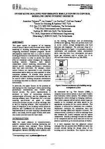
2.4.3 The Timing Routine The timing routine is at the heart of discrete-event simulation. From a programming perspective, this is the routine that ties the entire collection of processes together. The timing routine is transparent to the model builder. Let us define an “event” as a pending (re)activation of a process. Then the timing routine is as shown in figure 2-1.

START SIMULATION

ANY PROCESSES ON PENDING LIST?

NO

Yes

SELECT PROCESS WITH EARLIEST (RE)ACTIVATION TIME

RETURN

UPDATE CLOCK TO TIME OF EVENT

DETERMINE TYPE OF PROCESS

REMOVE PROCESS FROM PENDING LIST

EXECUTE PROCESS ROUTINE

Figure 2-1. Basic SIMSCRIPT II.5 Timing Routine As can be seen from the figure, processes must be on the pending list prior to entry into this routine or the simulation will terminate immediately. It is natural to assume that the execution of one process will (or may) activate other processes and thus perpetuate this

14


sequence for some time. Termination will occur either for the algorithmic reason shown in the figure or because some process executes a stop statement. 2.4.4 Process Routines Each process declared in the program preamble must be further described by a process routine. The names of the process object and process routine are identical. Continuing our analogy with play writing, a process routine is like the script for a single character. Or, if several characters do very similar things, we might think of the process description as a prototype description into which we plug different parameters. From a programming point of view, the process routine embodies the logic description of a process, telling what the process object does under all circumstances. Information pertinent to each process-instance is stored with the process notice telling, for example, the values of local variables in the routine, the time at which the process routine will next reactivate, the resources the process currently holds, and the reactivation point for the process-instance (a line number in the source code).

2.5 Example 1: A Simple Gas Station To solidify these concepts, let us construct a simple model and implement it in SIMSCRIPT II.5. Consider a small, full service gas station where customers arrive randomly, queue up for service, receive service, and leave. Our goal might be to determine the effects of adding or deleting gas pumps or attendants from the system. For the moment, however, our real goal is merely to construct and execute a very simple SIMSCRIPT II.5 model. To introduce randomness, assume that we have a source of uniformly distributed random numbers for which we can establish bounds. In SIMSCRIPT II.5 this is referenced as uniform.f . This function has three parameters: the lower bound, the upper bound, and a random number stream. Each time the function is executed, a new sample from the interval is computed. Refer to chapter 4 for the details on representing random phenomena. The customers are modeled as processes. Customers arrive, request service, wait if no server is available, occupy the server for awhile, and then depart. For this model, it is sufficient to model the attendant (server) as a resource. This program will be discussed in two phrases: first, a walk-through of the SIMSCIPT II.5 code presented in figure 2-2; and second, a walk-through of the sample execution is presented in Example 1.

15


1 2 3 4 5 6

'' EXAMPLE 1

A SIMPLE GAS STATION MODEL

1 2 3 4 5 6

main create every ATTENDANT(1) let U.ATTENDANT(1) = 2 activate a GENERATOR now start simulation end

1 2 3 4 5 6 7

process GENERATOR for 1 = 1 to 1000, do activate a CUSTOMER now wait uniform.f(2.0, 8.0, 1) minutes loop end

1 2 3 4 5

process CUSTOMER request 1 ATTENDANT(1) work uniform.f(5.0, 15.0, 2) minutes relinquish 1 ATTENDANT(1) end

preamble processes include GENERATOR and CUSTOMER resources include ATTENDANT end

Example 1. A Simple Gas Station Model Each segment of a SIMSCRIPT program begins with a keyword and ends with an end statement. In the preamble, two processes are declared, a GENERATOR (of new customers) and the CUSTOMER . The ATTENDANT (s) are modeled as a resource since a resource can be described passively. In the main program the initialization of resource ATTENDANT is accomplished by the create every statement, in which the number of “kinds” (or subgroups) of attendants is specified as one, and by the assignment statement, let . . . in which an automatically defined variable U.ATTENDANT is initialized to specify two units of attendant resources. That is, there are now two identical attendants who draw customers from a single queue. The activate statement creates a process object called GENERATOR and places it on the pending list with an immediate time of activation (now ). Start simulation passes control to the timing routine. Note that without this statement, no processes would ever be executed! Finally, in this model, when control returns from the timing routine (because all

16


processes are complete), control will pass immediately out of the program and back to the operating system. No output is produced from this model. An output will be added in paragraph 2-6. Each process is described as a separate routine which begins with a process statement naming the process. This name must correspond to one of the processes named in the preamble. The process GENERATOR contains a sequence of two statements, which are executed repetitively under the control of a simple iteration phrase for I = 1 to 1000. The statements do and loop delimit the scope of the for phrase. That is, statements between a pair will be executed 1000 times before the loop control logic is satisfied. Within the loop, the two statements create a new customer process object and place it on the pending list with an immediate time of activation. Then the wait statement puts the GENERATOR process object back on the pending list with a new reactivation time. The new time is determined by first drawing a sample from the population of real numbers between 2: and 8; (uniformly distributed), and then adding that value to the current “clock” time. The process CUSTOMER describes everything that happens to a customer from the time of arrival to the time of departure. This is very simple in this example. The customer requests an ATTENDANT. If neither ATTENDANT is available, the CUSTOMER process object is automatically placed on a list of objects waiting for the attendants. By default this list is ordered as “first-come-first-served.” The process is then suspended until this “blocking” condition (no available ATTENDANT ) is alleviated. When an ATTENDANT is available, one is assigned to this CUSTOMER and the CUSTOMER executes the work statement, which operates identically to the wait in GENERATOR except for the difference in distribution parameters. Finally, when the customer is reactivated after a period representing his service, the ATTENDANT is relinquish ed, either to be made available (if no CUSTOMERs are waiting) or to be allocated to the first CUSTOMER in the queue. This allocation automatically reactivates the other CUSTOMER, who will then execute his work statement. The present CUSTOMER is finished, so his process object is automatically destroyed and no trace remains of his ever having been in the system. In Example 1, the detailed execution is traced using the following notation: [Pi , n, t]

represents the ith instance of process P ready to resume execution at line n at time t. CUSTOMER s in queue have a time designated “*” to indicate that the time is unknown.

The progress of the program may be read from Example 1 in the following way. The current process is executed at its reactivation time and line. It continues executing, line by line, until it either encounters a delay (unavailable ATTENDANT or work/wait statement) or successfully completes execution. The system status recorded on the remainder of the line is after the process has progressed as far as possible without a time advance.

17


AFTER Current Process Executes Time

Current Process

Available Attendants

Customers in Queue

Pending Processes

0.0

[AT START SIMULATION]

2

none

[G1 ,1,0.0]

0.0

[G1 ,1,0.0]

2

none

[C1 ,1,0.0] [G1 ,6,7.547]

0.0

[C1 ,1,0.0]

1

none

[C1 ,4,6.847] [G1 ,6,7.547]

6.847

[C1 ,4,6.847]

2

none

[G1 ,6,7.547]

7.547

[G1 ,6,7.547]

2

none

[C2 ,1,7.547] [G1 ,6,10.617]

7.547

[C2 ,1,7.547]

1

none

[G1,6,10.617] [C2,4,14.400]

10.617

[G1 ,6,10.617]

1

none

[C3 ,1,10.617] [G1 ,6,14.073] [C2 ,4,14,400]

10.617

[C3 ,1,10.617]

0

none

[G1 ,6,14.073] [C2 ,4,14.400] [C3 ,4,24.367]

14.073

[G1 ,6,14.073]

0

none

[C4 ,1,14.073] [C2 ,4,14.400] [G1 ,6,21.932] [C3 ,4,24.367]

14.073

[C4 ,1,14.073]

0

[C4, 3, *]

[C2 ,4,14.400] [G1 ,6,21.932] [C3 ,4,24.367]

14.400

[C2 ,4,14.400]

0

none

[C4 ,3,14.400] [G1 ,6,21.932] [C3,4,24.367]

14.400

[C4 ,3,14.400]

0

none

[C4 ,4,20.143] [G1 ,6,21.932] [C3 ,4,24.367]

20.143

[C4 ,4,20.143]

1

none

[G1 ,6,21.932] [C3 ,4,24.367]

Example 1. Detailed Trace of Execution

18


For example, the one instance of the generator process, G1, is the first current process [G1, 1, 0.0]. After it has executed lines 1-5 of its process source code, the available ATTENDANT s and CUSTOMER s in queue are unchanged but two processes are now pending, the first CUSTOMER to enter the system (at time zero) and the GENERATOR itself which has drawn a first interarrival time delay of 7.547 minutes. It is important to observe the sequence in which these actions occur. In particular, let us clarify the meaning of now at the time of activation. The CUSTOMER process activated now in the GENERATOR is placed on the pending list and the GENERATOR process continues to execute until it, itself, is delayed (i.e., placed on the pending list) due to the execution of the wait statement. Thus, now means “as soon as control returns to the timing routine for next event selection.” Observe what happens when a process requests a resource of which no units are available. In Example 1 this occurs at time 14.073 when C4 is the current process. The process is placed on the “CUSTOMERS IN QUEUE” list. At this time it is not known when the resource will become available. This is represented by an asterisk in the time position. When the resource becomes available, in the example at [C2 ,4,14.400], it is immediately reallocated and the waiting process (C4) is moved from the queue to the pending process list. Notice that if C2 were to now re-request an ATTENDANT, C2 would be put on the CUSTOMERS IN QUEUE list, because the resource is no longer available.

2.6 Adding Performance Measurements Two measures that are commonly desired for this type of model are statistics on the queue (average, variance, maximum, etc.) and the utilization of the resources. These can be easily obtained in SIMSCRIPT II.5 by using the accumulate statement. The accumulate statement provides you with a simple means of specifying which measurements are desired without requiring detailed specification of the method of measurement. An accumulate statement is placed in the preamble. As the variable of interest changes during the course of the simulation, the system automatically captures the pertinent information. For example, consider the variable plotted in figure 2-3. This might represent queue length in our example.

19


VARIABLE

TIME

Figure 2-2. Time-Dependent Statistics Measurements of interest on this variable are time-dependent. The average value of the variable, for example, depends on how long the variable remains at a certain value. Two more automatically defined variables are available for use in our measurement task. Associated with each resource are counters indicating how many requests are currently being enqueued. As with the number of units variable, the names of these variables are derived from the name of the resource. They are N.X.resource and N.Q.resource, respectively. To display the results the print statement is introduced. The print statement consists of three parts: the keyword print and a specification of the number of lines of output to be produced from a single execution of the statement, a list of variable to be printed, and finally, a format or “picture” of output to be produced. This picture consists of text material to be printed verbatim, together with formats for the numerical data. There must be a oneto-one correspondence between elements in the list of variables and the formats. A numerical format is composed of a sequence of asterisks and, at most, one period. The number of asterisks after the decimal point governs the number of significant digits to be printed, with automatic rounding in the last position. The number of asterisks before the decimal point determines the maximum value that can be printed. However, automatic provision is made for blanks immediately preceding such a format to be treated as asterisks. Provision is also made for automatically detecting any overflow condition. Example 1A contains the completed program, including provision for measuring queue length and ATTENDANT utilization and for reporting these results. It should be observed that the only changes to the model from figure 2-2 are the addition of two accumulate statements in the preamble and the print statement in main. The value printed as utilization of the ATTENDANT s is the average value of N.X.ATTENDANT(1) divided by two, since the number of busy ATTENDANT s ranges from zero to two and it is desired to report their utilization as a percentage of possible utilization.

20


The placement of the print statement after the start simulation in main causes the output to be produced only after all processes activated in the model have terminated. Another possibility is to place the print statement after the loop statement in the GENERATOR process. This would have the effect of not including the wrap-up operation (i.e., serving customers after the door has been closed to new customers.) The results produced by executing the program in Example 1A are illustrated in Example 1A Output. 1 '' Example 1 A Example 1 with Performance Measurements Added 2 3 preamble 4 processes include GENERATOR and CUSTOMER 5 resources include ATTENDANT 6 accumulate AVG.QUEUE.LENGTH as the average 7 and MAX.QUEUE.LENGTH as the maximum 8 of N.Q.ATTENDANT 9 accumulate UTILIZATION as the average of N.X.ATTENDANT 10 end

1 main 2 create every ATTENDANT(1) 3 let U.ATTENDANT(1) = 2 4 activate a GENERATOR now 5 start simulation 6 print 4 lines with AVG.QUEUE.LENGTH(1), MAX.QUEUE.LENGTH(1), 7 and UTILIZATION(1) * 100. / 2 thus SIMPLE GAS STATION MODEL WITH 2 ATTENDANTS AVERAGE CUSTOMER QUEUE LENGTH IS *.*** MAXIMUM CUSTOMER QUEUE LENGTH IS * THE ATTENDANTS WERE BUSY **.** PER CENT OF THE TIME. 8 end

1 2 3 4 5 6 7

process GENERATOR for I = 1 to 1000 do activate a CUSTOMER now wait uniform.f(2.0,8.0,1) minutes loop end

1 2 3 4 5

process GENERATOR request 1 ATTENDANT(1) work uniform.f(5.0,15.0,2) minutes relinquish 1 ATTENDANT(1) end

Example 1 with Performance Measurements Added

21


SIMPLE GAS STATION MODEL WITH 2 ATTENDANTS AVERAGE CUSTOMER QUEUE LENGTH IS 7.809 MAXIMUM CUSTOMER QUEUE LENGTH IS 21 THE ATTENDANTS WERE BUSY 98.64 PER CENT OF THE TIME.

Example 1A Output

2.7 A Slightly More Complicated Example One of the goals in modeling is to explore alternatives in design. This may entail including more (or less) detail than originally anticipated, changing numerical data in the model, or including more measurement requirements. To illustrate the ease of doing this in SIMSCRIPT II.5, the model will be modified as follows: a. Customers choose whether they require premium or regular gas. They must wait for the proper pump to become available. Let us arbitrarily assume that 70% require premium and 30% require regular. Initially, we will arbitrarily have one regular pump and three premium pumps. b. An attendant is not required until the pump is available. The attendant starts the pump and then is free until the pump stops. He is then required in order to complete the service. c. The queues and utilization for the attendants and two types of pumps will be measured. Example 2 shows the program modified to incorporate these features. The program shows three features of SIMSCRIPT II.5 not used previously: • • •

define to mean

local variables simple decision logic

2.7.1 Define to Mean In the interest of improved readability of programs, SIMSCRIPT II.5 allows you to substitute a character string for a single word, and thus to develop your own vocabulary or shorthand notation. The general form of the statement is: define WORD to mean STRING

A constraint is that STRING must be confined to a single input record. In the example this feature allows mnemonic values for our pump resource subscripts (.REGULAR or .PREMIUM ). It is purely a style convention in this example to have every define to mean symbol begin with a period.

22


1 ''EXAMPLE 2 A MORE ELABORATE GAS STATION MODEL 2 3 preamble 4 processes include GENERATOR and CUSTOMER 5 resources include ATTENDANT and PUMP 6 accumulate AVG.ATTENDANT.QUEUE.LENGTH as the average 7 and MAX.ATTENDANT.QUEUE.LENGTH as the maximum 8 of N.Q.ATTENDANT 9 accumulate UTILIZATION as the average of N.X.ATTENDANT 10 accumulate AVG.PUMP.QUEUE.LENGTH as the average 11 and MAX.PUMP.QUEUE.LENGTH as the maximum 12 of N.Q.PUMP 13 accumulate PUMP.UTILIZATION as the average of N.X.PUMP 14 define .REGULAR to mean 1 15 define .PREMIUM to mean 2 16 end

1 main 2 create every ATTENDANT(1) 3 let U.ATTENDANT(1) = 2 4 create every PUMP(2) 5 let U.PUMP(.REGULAR) = 1 6 let U.PUMP(.PREMIUM) = 3 7 activate a GENERATOR now 8 start simulation 9 print 10 lines with AVG.ATTENDANT.QUEUE.LENGTH(1), 10 MAX.ATTENDANT.QUEUE.LENGTH(1), 11 UTILIZATION(1) * 100. / U.ATTENDANT(1), 12 AVG.PUMP.QUEUE.LENGTH(.REGULAR), MAX.PUMP.QUEUE.LENGTH(.REGULAR), 13 PUMP.UTILIZATION(.REGULAR) * 100. / U.PUMP(.REGULAR), 14 AVG.PUMP.QUEUE.LENGTH(.PREMIUM), MAX.PUMP.QUEUE.LENGTH(.PREMIUM), 15 PUMP.UTILIZATION(.PREMIUM) * 100. / U.PUMP(.PREMIUM) thus SIMPLE GAS STATION WITH TWO ATTENDANTS AND TWO GRADES OF GASOLINE AVERAGE QUEUE WAITING FOR ATTENDANTS IS *.*** CUSTOMERS MAXIMUM “ “ “ “ * THE ATTENDANTS WERE BUSY *.** PER CENT OF THE TIME. THE QUEUES FOR THE PUMPS WERE AS FOLLOWS: GRADE AVERAGE MAXIMUM UTILIZATION REGULAR *.*** * *.** PERCENT PREMIUM *.*** * *.** PERCENT 16 end

Example 2. A More Elaborate Gas Station Model

23


1 2 3 4 5 6 7

process GENERATOR for I = 1 to 1000 do activate a CUSTOMER now wait uniform.f(2.0,8.0,1) minutes loop end

1 process CUSTOMER 2 define GRADE as an integer variable 3 if random.f(3) > 0.70, 4 let GRADE = .REGULAR 5 else 6 let GRADE = .PREMIUM 7 always 8 request 1 PUMP(GRADE) 9 request 1 ATTENDANT(1) 10 work uniform.f(2.0,4.0,2) minutes 11 relinquish 1 ATTENDANT(1) 12 work uniform.f(5.0,9.0,2) minutes 13 request 1 ATTENDANT(1) 14 work uniform.f(3.0,5.0,2) minutes 15 relinquish 1 ATTENDANT(1) 16 relinquish 1 PUMP(GRADE) 17 end

Example 2. A More Elaborate Gas Station Model - Continued

SIMPLE GAS STATION WITH TWO ATTENDANTS AND TWO GRADES OF GASOLINE AVERAGE QUEUE WAITING FOR ATTENDANTS IS .138 CUSTOMERS MAXIMUM “ “ “ 2 THE ATTENDANTS WERE BUSY 69.93 PER CENT OF THE TIME. THE QUEUES FOR THE PUMPS WERE AS FOLLOWS: GRADE AVERAGE MAXIMUM REGULAR: 1.237 8 PREMIUM: .084 3

Example 2. Output

24

UTILIZATION 79.94 PERCENT 70.74 PERCENT


2.7.2 Local Variables The variables used so far have been global in scope. That is, the same variable can be referenced from anywhere in the program. For example, the variable U.ATTENDANT was initialized in main and modified in the execution of the request and relinquish statements in the process CUSTOMER . It is sometimes necessary to define variables which are private to a particular process, or even more specifically, to an individual instance of a process. This is accomplished by defining local variables in the body of a process. For example, in the model, it is necessary that each customer “remember” which grade of gasoline they want, so that when they have been served they can relinquish the proper pump. This is accomplished by defining the variable GRADE within the process CUSTOMER. 2.7.3 Simple Decision Logic The final new concept introduced in this model is the ability to alter the flow of control explicitly in the program logic. The if statement is used to describe two alternative courses of action. The form of the statement is: if logical test group of statements1 else group of statements2 always

and it is executed in this manner. The logical test is evaluated. It will be either true or false. If it is true, group of statements 1 will be executed and group of statements 2 will not. If the logical test is false, only group of statements2 will be executed. In either case the statements which follow the word always are executed. In this example, this construct is used to randomly select the grade of gasoline for each customer. Random.f(i) is a function that uses the ith random number stream to return a value sampled from the population uniformly distributed between 0 and 1. This value should be less than 0.70 seventy percent of the time, corresponding to our estimates of the number of customers who use premium grade. The results from executing this model are displayed in Example 2 Output. This more realistic model shows the breakdown of congestion between pump demands and attendant demands. However, the data are purely fictitious and no significant conclusions should be drawn without more analysis of the situation. 2.7.4 Concluding Remarks This chapter has introduced many of the modeling concepts supported by the SIMSCRIPT II.5 language. Many problem areas can be addressed by analogy to the models presented. About 25% of the statements of the language have been illustrated. But, almost without

25


exception, each of the statements has more complex forms or alternative applications. Succeeding chapters go into much more detail. The chapters will show how these constructs may be elaborated upon in some instances and dissected in others, for purposes of greater understanding or for use in nonstandard applications. For those readers who desire a more formal treatment of the language than this tutorial permits, Appendix A contains a formal syntax of all the statements of the SIMSCRIPT II.5 language. Appendix B summarizes the coding and style conventions used in the examples. Appendices C and D give all the particulars about system-defined variables, functions, and routines.

26

3. Modeling Individual Objects 3.1 Attribute Concept In Chapter 2 the system was modeled without the need to identify individual copies of objects explicitly. Objects often must be described in more detail. Processes and resources can be given attributes. In fact, some attributes of resources were used in Chapter 2. However, these attributes were defined by the system. The number of units of a resource, the number of outstanding requests, and the number of currently satisfied requests are all contained in attributes of a resource. You may add as many attributes as you choose to characterize the resources adequately. For example, instead of remembering that the first PUMP subgroup is for regular gas and the second is for premium, you may choose to have a type or GRADE attribute. In addition, you might wish to keep track of the remaining reserve of each GRADE. To add these features write: resources every PUMP has a GRADE

When space is allocated for this resource, the data structure can be represented as shown in figure 3-1. create every PUMP (3)

1

2

3 U.PUMP N.X.PUMP N.Q.PUMP GRADE

Figure 3-1. Pump Resource Data Structure Each column in the figure represents the storage for the attributes of a different pump group. Two more variables are automatically associated with each resource. One is a variable with the same name as the resource; the other is a variable whose name is derived from the resource name by prefixing “N. ”. N.resource is used as a reference to a particular object (or column in figure 3-1). Thus, in the example N.PUMP has a value of 3, taken from the create statement. The initial value of all SIMSCRIPT variables is zero. Therefore, before using the variable PUMP we must initialize it to a valid value—in this case 1, 2, or 3.

27


We use the entity name like a subscript and refer to specific attributes as GRADE(PUMP) or “grade of pump.”

3.2 Variables Several SIMSCRIPT II.5 variables have been used in previous examples without a precise definition of their characteristics. These variables will now be given definitions of their characteristics. SIMSCRIPT II.5 variables are of numerous types. Attributes, reference variables, and simple variables are only a few of the types available, but they will suffice to introduce the concepts. Variables are either global or local in scope. A global variable must be defined in the program preamble. If a variable is not explicitly defined anywhere, it becomes a local variable by default, provided that it is used in proper context. All variables have a mode which may be integer, double, real, alpha , or text. Double is the background or default mode. That is, if a variable is defined implicitly or even explicitly without specifying a mode, it assumes the background mode. background mode may be changed by use of the statement:

The

normally, mode is mode

If this statement appears in the preamble , it has the effect of changing the background for the remainder of the preamble and all programs compiled with the preamble. It may, of course, be superseded by subsequent normally statements. If a normally statement appears in an individual routine, it applies only to variables in that routine. It is better programming practice to define every variable explicitly and not to rely on the system defaults. 3.2.1 Global/Local Conflicts A variable which is defined in the preamble (and is thus global) may also be defined explicitly in an individual routine. When this is done, the global variable is effectively excluded from use in that routine. This is particularly useful in isolating or eliminating “side effects” of the execution of routines. This will be illustrated in figure 3-4. A variable is initialized to zero automatically when the storage for the variable is allocated. For a global variable, this occurs at the beginning of the execution of the program. For a local variable in a routine or process, the local variable is allocated upon entry into the routine. Local variable storage remains allocated until the routine “ends.” For a routine this means at the execution of a return statement. The execution of process delaying statements does not cause local storage to be deallocated. The local storage for a process remains allocated until the process is finally completed. Note that this method of storage allocation provides each copy of a process with its own local storage and also permits recursive calls of routines.

28

Chapter 3. Modeling Individual Objects

3.2.2 Naming of Variables You have great freedom in naming variables. The only restriction on name length is that it must be contained within a single record of input to the compiler. A single record is typically 80 characters. The SIMSCRIPT II.5 keywords are not reserved words and thus may be used as variable names. However, this feature should not be used, because it creates unreadable programs. A variable name is any sequence of letters, digits, and periods that does not form a number. ABC, NO.OF.CUSTOMERS, 4F, 5.12.38, 1E6 and ABC... are all valid names. 1., 567, 2+2 and 5.12 are not valid names. They are numbers or expressions. The compiler drops terminal periods in names. Thus, ABC and ABC... are representations of the same variable name. SIMSCRIPT II.5 contains many predefined variables and constants, as well as automatically generated variables. They are named as shown in table 3-1.

Table 3-1. Naming Conventions for Variables Category

Form

Examples

Meaning

Constants

name.c

pi.c

π

Variables

NAME.V

TIME.V HOURS.V

simulation clock number of hours/day

Functions

name.f

sqrt.f uniform.f

square root uniform random deviate generator

Generated Attributes

letter.name

u.pump n.q.pump

units attribute of a resource number in queue for a resource

By SIMSCRIPT II.5 language rules, system names (of the form NAME.LETTER) and generated names (of the form LETTER.NAME) are used only for purposes defined by the language implementation. Appendix D describes the system names.

3.3 Arithmetic SIMSCRIPT II.5 uses the usual operators and precedence rules. Parentheses are used to change the order of evaluation, forcing evaluation of expressions within parentheses before using the result in outer expressions. There is no limit to the length of an expression or the depth of nesting of parentheses. For example, let A = B+D/(C-E*F)**2

is evaluated as follows:

29


1. 2. 3. 4. 5. 6.

Multiply E by F. Subtract the product from C. Square the difference. Divide D by the result of 3. Add B. Store the result in A.

3.4 Data Input Models are usually constructed to perform parametric studies. Typically, a wide range of values need to be tested and the specific values or sequence of values are not known a priori. Rather than build constant values into a model and then require recompilation each time one value needs to be changed, it is common practice to provide for parameters to be changed at the time of execution of the model, without change to the source code. The freeform read statement is used for this purpose. read X, N.TELLER, U.PUMP (1)

The read statement consists of the keyword read followed by a list of variables separated by commas. The format of the data is not specified in the statement but rather is implied by the language. The implied format is that a sequence of data fields will be read corresponding to the variables in the read statement. A data field is a sequence of non-blank characters. It is terminated by either a blank or the end of a record. A single read statement may use several records to satisfy its input data requirements. A read statement does not automatically start a new record. Thus, if successive read statements are executed, the first one might read several entire records and part of one more. The second read will read any data fields on the current record before starting a new record. If there is disagreement between the mode of the data field and the mode of the variable, conversion will be made automatically where the conversion is permitted. The allowable conversions are shown in figure 3-2.

30


Variable Mode

Form of Data

 Integer   Real   Characters

Integer

Real

Alpha

Text

Integer

Real

Alpha

Text

X

Real

Alpha

Text

X

X

Alpha

Text

where X denotes an error condition.

Figure 3-2. Input Data Mode Conversions The mode of an input data field is determined in the following manner: 1. A sequence of digits, possibly including a preceding sign, is regarded as integer. 2. A sequence of digits (that may have a sign) with a decimal point is regarded as real . In addition, scientific notation is recognized as real . It consists of a real representation plus an exponent in the form: SXX.XXESXX

where S represents an optional sign, X represents a digit, and E is an optional separator between fraction and exponent (either E or the sign of the exponent is required). 3. Anything else is regarded as an alpha or text mode string.

3.5 Program Control Structures There are several statements in SIMSCRIPT II.5 for altering the flow of program control. The if statement in its most general form was used in figure 2-5, and a simple loop structure was used to control the generation of new customers. 3.5.1 IF Statement Sometimes the full structural power of the if statement is not needed to describe a branching condition. For example, when a block of statements is executed conditionally, but no alternative is needed other than to execute those statements, the else can be omitted. For example, if STATUS = BUSY add 1 to BACK.LOG always

31


On the other hand, the first path may end with an unconditional transfer of control such as stop or return. In this case, the alternative is the remainder of the routine and no always is needed. The always should not be included in this case, as it may cause another if structure to be terminated. If structures can be nested to any depth. if BACK.LOG = 0 let STATUS = IDLE return otherwise

3.5.2 Looping The indexed for phrase used previously for simple counter control can also be applied to a resource entity in the following manner: for each resource

is equivalent to: for resource = 1 to N.resource

In this example, resource is a defined resource entity. This illustrates that the variable associated with each resource is incremented over its range of valid values from one to the number of subgroups of the resource ( N.resource). An alternative form of this phrase is: for each resource called name

which is equivalent to: for name = 1 to N.resource

It is often desirable to be selective in this searching operation. For this purpose it is possible to build into the control structures phrases for specifying conditions which must be met either to include or exclude a certain case, or conditions for continuing or terminating the search. The logical comparisons that may be used in these phrases are the same as those used in the if statement. They include: equality inequality less than greater than

= ¬ = < >

eq ne lt gt

and combinations of these. For program readability, a large collection of synonyms is available. See Appendix A.

32


Each logical expression will be evaluated to a true or false value. In addition to these simple expressions, compound expressions may be composed by using the logical connectives, and, or, and parentheses. For example, you might need a certain combination of attribute values on a resource to exist before the resource is of use. For example, for each PUMP with GRADE(PUMP) = DESIRED.GRADE and RESERVE(PUMP) >= 10.0 find the first case

specifies a search over all the PUMP resource subgroups, looking for the first one that has a GRADE attribute whose value matches a desired grade, and simultaneously has a value greater than or equal to 10 in its reserve attribute. The find statement causes the search to terminate on the first success. It may be followed, optionally, by an if statement to determine the outcome. The format of this statement is if found , or alternately, if none. Sometimes the search is for the maximum or minimum over all the subgroups. In this case, the compute statement is used in place of the find statement, since it is necessary to look at all cases before ascertaining that the maximum or minimum has indeed been found. As an example, for each TELLER, compute SHORTEST.QUEUE.LENGTH as the minimum of N.Q.TELLER(TELLER)

will examine the N.Q.TELLER attribute of each subgroup of TELLERs and records, as the value of the variable SHORTEST.QUEUE.LENGTH, the minimum value of this attribute among all the TELLER subgroups. Often, it is not the value of the variable that is important, but rather the index corresponding to the value that maximizes or minimizes the variable. To record the index, a slightly different form of the statement is used: for each TELLER, compute SHORTEST.QUEUE as the minimum(TELLER) of N.Q.TELLER(TELLER)

This is interpreted as “Examine the value of the length attribute of each TELLER queue and record in SHORTEST.QUEUE , the value of the index TELLER for which this variable is a minimum.”

33


3.6 Representation of Time We have used time expressions in our simulation models without precisely describing the representation of time internally to the system. The SIMSCRIPT II.5 simulation “clock” is a system-defined, real variable called TIME.V. Initially, TIME.V has a value of zero, although it may be initialized to any starting value. The default units for time are days. If time expressions are given in hours or minutes, appropriate adjustments are made using two system-defined variables, HOUR.V and MINUTES.V . The default values for these variables are 24 and 60, respectively, indicating the expected conversions of 24 hours per day and 60 minutes per hour. You may change these values to represent, for example, an eight hour day. In combination with the define to mean feature, the entire time domain may be easily changed. For example, in modeling computer systems it is often convenient to represent times in units of seconds, milliseconds, and microseconds. While these words are not a part of the SIMSCRIPT vocabulary, they may be added as shown here: preamble define .SECONDS to mean DAYS define .MILLISECONDS to mean HOURS define .MICROSECONDS to mean MINUTES end main let HOURS.V = 1000 let MINUTES.V = 1000 end

Now statements such as wait 32 .MILLISECONDS can be written. Note, however, that the conventional meanings of days, hours, and minutes have been substantially altered! The timing routine, as noted in Chapter 2, updates TIME.V as it causes the simulation to progress. It should be noted that any attempt to retrogress in simulated time causes a terminal error in the execution of the model.

3.7 Time Measurements In paragraph 2-6 it was seen that it is often necessary to measure phenomena as they change over simulated time. There are also many measures which are not time-dependent, but rather depend on the number of samples taken. Actually, all measures could be performed by taking samples, but using the accumulate statement is much more convenient. The tally statement is used with sample-based measurements. Like the accumulate statement, it is a declarative statement appearing in the preamble. There are many applications of the tally statement. Many involve sampling time measurements such as delays, actual service times, total cycle time, etc.

34


Figure 3-3 illustrates an example of measuring the waiting time of the first several customers in a system.

Waiting Time

Customer Number

Figure 3-3. Time-Independent Statistics Notice that zero waiting times are explicitly recorded as sample values in order to be included in the statistics. If the default time values are used, these measurements will be recorded in units of days. The results may be converted to hours or minutes by using the system variables HOURS.V and MINUTES.V.

3.8 Example 3: A Bank With a Separate Queue for Each Teller All of the features discussed so far in this chapter will now be illustrated by modeling a bank in which customers arrive, go immediately to any available teller, receive service, and leave. If all tellers are busy, the arriving customer joins the shortest line, and waits there until served. While it is an unreasonable assumption that customers remain in one line when another teller becomes available, it will give an extreme value for comparing this model to the newer-style bank in which all customers form a single line to be served by the next available teller. When jockeying is permitted, the single line is the optimum equivalent. The measures required are the average and maximum queues, the utilization of each separate teller, and the mean waiting time for all customers. 3.8.1 Model Formulation This system will be modeled using two processes and one resource. The GENERATOR process will inject customers into the system with an exponential distribution of interarrival times until a pre-specified closing time. The model will terminate after all customers who arrived before closing time finish being served. Chapter 4 provides details on exponential distribution.

35


The CUSTOMER process will contain the complete description of the actions of one customer from arrival at the bank until departure. The single resource, TELLER, is used with the subgroup concept—one subgroup per individual TELLER—so as to easily accomplish the separate queueing and measurements. Certain model parameters are explicitly defined as global variables to permit initializing them in one program ( main ) and using them in another (process GENERATOR and CUSTOMER). The program listing for this example is shown in Example 3.

36


1 '' Example 3 A Bank With Separate Queues for Each Teller 2 3 preamble 4 processes include GENERATOR and CUSTOMER 5 resources include TELLER 6 define MEAN.INTERARRIVAL.TIME, MEAN.SERVICE.TIME, 7 DAY.LENGTH and WAITING.TIME as real variables 8 9 accumulate UTILIZATION as the average of N.X.TELLER 10 accumulate AVG.QUEUE.LENGTH as the average, 11 MAX.QUEUE.LENGTH as the maximum of N.Q.TELLER 12 tally MEAN.WAITING.TIME as the mean of WAITING.TIME 13 end 1 main 2 read N.TELLER, MEAN.INTERARRIVAL.TIME, MEAN.SERVICE.TIME 3 and DAY.LENGTH 4 create every TELLER 5 for each TELLER, 6 LET U.TELLER(TELLER) = 1 7 print 8 lines with N.TELLER, MEAN.INTERARRIVAL.TIME, 8 MEAN.SERVICE.TIME and DAY.LENGTH thus SIMULATION OF A BANK WITH * TELLERS (EACH WITH A SEPARATE QUEUE) CUSTOMERS ARRIVE ACCORDING TO AN EXPONENTIAL DISTRIBUTION OF INTER ARRIVAL TIMES WITH A MEAN OF *.** MINUTES. SERVICE TIME IS ALSO EXPONENTIALLY DISTRIBUTED WITH A MEAN OF *.** MINUTES. THE BANK DOORS ARE CLOSED AFTER *.** HOURS. (BUT ALL CUSTOMERS INSIDE ARE SERVED.) 9 10 activate a GENERATOR now 11 start simulation 12 13 print 6 lines with TIME.V * HOURS.V, 14 and MEAN.WAITING.TIME * HOURS.V * MINUTES.V thus THE LAST CUSTOMER LEFT THE BANK AT *.** HOURS. THE AVERAGE CUSTOMER DELAY WAS *.** minutes. TELLER

15 16 17

UTILIZATION

QUEUE LENGTH AVERAGE MAXIMUM

for each TELLER, print 1 line with TELLER, UTILIZATION(TELLER), AVG.QUEUE.LENGTH(TELLER), MAX.QUEUE.LENGTH(TELLER) thus *.** *.** *

* 18 end

Example 3. A Bank With a Separate Queue for Each Teller

37


1 2 3 4 5 6 7 8 9

process GENERATOR define TIME.TO.CLOSE as a real variable let TIME.TO.CLOSE = DAY.LENGTH / HOURS.V until TIME.V >= TIME.TO.CLOSE, do activate a CUSTOMER now wait exponential.f(MEAN.INTERARRIVAL.TIME, 1) minutes loop end

1 process CUSTOMER 2 define ARRIVAL.TIME as a real variable 3 define MY.CHOICE as an integer variable 4 let ARRIVAL.TIME = TIME.V 5 for each TELLER, with N.X.TELLER(TELLER) = 0, 6 find the first case 7 if found, 8 let MY.CHOICE = TELLER 9 else 10 for each TELLER, 11 compute MY.CHOICE as the minimum(TELLER) 12 of N.Q.TELLER(TELLER) 13 always 14 request 1 TELLER(MY.CHOICE) 15 let WAITING.TIME = TIME.V - ARRIVAL.TIME 16 work exponential.f(MEAN.SERVICE.TIME,2) minutes 17 relinquish 1 TELLER(MY.CHOICE) 18 end

Example 3. A Bank With a Separate Queue for Each Teller Continued SIMULATION OF A BANK WITH 2 TELLERS (EACH WITH A SEPARATE QUEUE) CUSTOMERS ARRIVE ACCORDING TO AN EXPONENTIAL DISTRIBUTION OF INTER ARRIVAL TIME WITH A MEAN OF 5.00 MINUTES SERVICE TIME IS ALSO EXPONENTIALLY DISTRIBUTED WITH A MEAN OF 10.00 MINUTES. THE BANK DOORS ARE CLOSED AFTER 8.00 HOURS. (BUT ALL CUSTOMERS INSIDE ARE SERVED.) THE LAST CUSTOMER LEFT THE BANK AT 9.49 HOURS. THE AVERAGE CUSTOMER DELAY WAS 19.84 MINUTES. TELLER 1 2

UTILIZATION .97 .91

QUEUE LENGTH AVERAGE MAXIMUM 1.73 6 2.06 7

Example 3. Output

38


3.8.2 Program Discussion For the sample execution shown in Example 3 Output, the input data could have been prepared as: 2

5.0

10.

8

A more elaborate model might request this information in an interactive dialog. A good programming practice is to print all the input data so as to verify that no miscommunication has occurred. This is shown in main. This model is designed to terminate by running out of active processes and returning control to main for final analysis output. The process CUSTOMER has the following salient features: a. Lines 2, 4 and 15 compute a sample of waiting time for each CUSTOMER. b. Lines 2 and 3 define local variables in order to preserve a record for each CUSTOMER of the time of arrival and the selected TELLER . Preserving a record of the selected TELLER is imperative, so that after a time delay either for queueing, service, or both, the proper TELLER resource will be relinquished. c. The CUSTOMER decision making function is broken into two steps: 1. Look for the idle TELLER (lines 5-8); 2. If no idle TELLER is found, look for the shortest line (lines 10-12). This operation could have been combined into a single search of the form: for each TELLER compute MY.CHOICE as the minimum(TELLER) of N.X.TELLER(TELLER)+N.Q.TELLER(TELLER)

The process GENERATOR is slightly different from previous examples in that the number of CUSTOMERs to be generated is not specified, but rather a time at which to stop generating them. The until phrase is another loop variant. This time there is no need for the for phrase. There is a slight imprecision in this model-closing procedure in that, if there were no customers in the bank at closing time, the model would not actually stop and summarize statistics immediately, but would only do so at the time of next CUSTOMER arrival since that is the time at which the process GENERATOR would be terminated. This can be remedied with additional commands that will be discussed in the next paragraph.

3.9 Process Attributes Attributes may be associated with processes as well as resources. For example, it might be necessary to carry along as attributes of the process CAR such information as the time of

39


arrival, the grade of gasoline required, and the amount of gasoline required. These can all be defined in a statement such as: processes every CAR has a TIME.OF.ARRIVAL and a GAS.GRADE and a TANK.CAPACITY

When such a process is activated, these attributes will automatically be initialized to zero. In order to assign values later, the attribute is associated with the particular process through the use of a reference variable, sometimes called a pointer variable. For example, let TANK.CAPACITY(CAR) = 15

This statement is read as “let TANK.CAPACITY of CAR be set equal to fifteen.” The variable CAR is a reference variable. Its value is established by the activate statement. activate a CAR in 10 minutes

which is now seen to mean: 1. Create a process notice to describe a new CAR . 2. Place the reference value for this notice in the variable CAR. 3. Compute the time at which this activation will take place (current time + ten minutes) and store this value as an attribute of the process. 4. Place the process notice in the pending list.

40


Only one CAR process notice is accessible by this mechanism at any particular time. It is possible to refer to more than one copy of processes of the same class in the following manner: activate a CAR called X in 5 minutes activate a CAR called Y in 10 minutes let TANK.CAPACITY(X) = 17 let TANK.CAPACITY(Y) = 20

This concept is summarized in figure 3-4.

X

CAR

Y

TIME.OF.ARRIVAL

0

0

0

GAS.GRADE

0

0

0

TANK.CAPACITY

0

17

20

. . .

. . .

. . .

Figure 3-4. Multiple Process Data Structures Each process notice has space for the defined attributes plus some additional systemdefined information to be discussed later. These process notices are dynamically allocated blocks of storage. You do not need to be concerned with where they are stored, how many are allocated at any particular time, or the order of assignment of the attributes to the words within the process notice. The variable with the generic name of the process becomes, by default, a global variable— accessible from any part of the model—whereas other variables default to a local context.

41


The attributes of a process can be initialized as part of the execution of the activate statement. Assume, for example, that we have a process representing a message in a communications network defined as follows: processes every MESSAGE has an ORIGIN and a DESTINATION

We might represent a message to be sent from Los Angeles to Washington, D.C. as: activate a MESSAGE giving LA and DC now

This is equivalent to the following sequence of statements: create a MESSAGE let ORIGIN(MESSAGE) = LA let DESINATION(MESSAGE) = DC activate this MESSAGE now

This latter breakdown illustrates two further concepts: the ability to create a process notice without placing it in the pending list; and then, later on, activating the process without automatically creating a new process notice. The distinction in the form of the activate statement is very subtle. The indefinite article (a or an) is replaced by a definite article (the or this ). The values in the giving phrase are assigned to attributes in the order in which the attributes were defined in the preamble.

3.10 Argument Passing for Subroutines When a subroutine is invoked, it is often necessary to pass information to that routine. Upon completion, the subroutine communicates its results to the calling routine via arguments. In SIMSCRIPT II.5, the given information and the results are passed as separately specified arguments. A subroutine is invoked via the call statement. For example, call HARBOR.MASTER giving SHIP and “ARRIVING” yielding STATUS

specifies invocation of the routine named HARBOR.MASTER, passing to it as arguments the value of the variable SHIP and the literal “ARRIVING.” The result of this execution of the routine will be placed in the variable STATUS. The corresponding procedure declaration heading might appear as: routine HARBOR.MASTER giving NEW.SHIP and ACTION yielding STATUS define NEW.SHIP and STATUS as integer variables define ACTION as a TEXT variable

Note: The arguments must agree in mode and in number between the call statement and the routine declaration.

42


3.11 Subprogram Variables The subprogram variable is a generalization of the subroutine calling mechanism. A subprogram variable is declared as, for example: define DEBUG as a subprogram variable

or, define TRIG as a real subprogram variable

When a mode is specified, it refers to the mode of the result of the subprogram when called as a function. This will be illustrated below. To initialize a subprogram variable, a let statement must be used to assign a subprogram literal as the value of the variable. For example, let TRIG = 'sin.f'

The subprogram literal may be any SIMSCRIPT library routine or a routine written by the user. A statement such as: let B = TRIG

would copy the address of the sin.f function to another subprogram variable, B, whereas: let X = $TRIG(.5)

would compute the value of sin.f(.5) and store the result in X. This presents a syntactic problem. Since a subprogram variable can be subscripted, i.e., an array or an attribute, what does the quantity in parentheses represent? The answer is that it is the argument to the routine. If it is necessary to execute a subprogram stored in an array or attribute, it must first be moved to an unsubscripted subprogram variable. For example: processes every PORT has a PT.ROUTINE define PT.ROUTINE as a subprogram variable . . . process PORT define LOCAL as a subprogram variable store PT.ROUTINE in LOCAL call LOCAL giving PORT . . .

43


This program illustrates that a different routine can be associated with each different process instance, i.e. each port, to be called from the process when needed.

3.12 Argument Passing for Processes It is not necessary to explicitly pass arguments to processes, since the values of the arguments are taken from the attributes of the process notice. They may be referenced directly. However, it is occasionally convenient or more natural to specify parameters for a process. Only given parameters may be specified for processes. The arguments (or formal parameters) take their values from the user-defined attributes specified in the process notice definition in the preamble. It is not necessary to provide arguments for all of the attributes. However, the attributes will be assigned to the arguments in the order of preamble definition. The mode-mismatch problem of subroutines does not arise for processes. However, process attributes are copied to the arguments only upon initial entry to the process routine. If, for some reason, the attribute values are changed while the process is either active or passive (i.e., from within or without the process), this will have no effect on the argument values. For example, consider the previous MESSAGE process example. With the same preamble definition and activate statement: processes every MESSAGE has an MG.ORIGIN and an MG.DESTINATION activate a MESSAGE giving LA and DC now

The process routine might start with, process MESSAGE given ORIGIN and DESTINATION define ORIGIN and DESTINATION as integer variables

It is not permissible to use the same variable names as process attributes and process routine arguments. The common solution is to give the desired name to the argument and prefix the attribute with a reminder of the process name (e.g., ORIGIN versus MG.ORIGIN ). The process attribute names may not even appear in the program because of the giving phrase in the activate statement.

3.13 Process Interaction Commands We have seen two types of process interactions thus far: a. A process activates another process (via the activate statement). b. A process restarts another process by relinquishing a resource that the later process has requested. Several more process interaction commands may be used to describe direct communication between processes. They allow for:

44


a. Interrupting a process that is currently awaiting time passage, as in a work or wait statement. b. Resuming a process previously interrupted. c. Suspending a process (this statement applies only to the currently executing process—a short of “do it yourself” command). d. Destroying a process. All of these interactions are summarized in the state transition diagrams of figures 3-5 and 3-6.

AC

CREATED

EA CR

TIV AT E

TE

ST DE

I NT

Y RO

ER R

“TH

E” R

ES UM

E

UP T

ACTIVATE “A” ACTIVE

NONEXISTENT

L RE

QU IN

H IS

DELAYED FOR RESOURCE

Legend: Solid lines represent immediate actions. Dotted lines represent simulation time-delayed actions.

Figure 3-5. Actions Performed for a Process (External to the Process, Itself)

45


CREATED

SU SP EN

D W

W

NONEXISTENT

RETURN

OR AI K T

ACTIVE

END QU RE

T ES

DELAYED FOR RESOURCE

Legend Solid lines represent immediate actions. Dotted lines represent simulation time-delayed actions.

Figure 3-6. Actions a Process Performs for Itself 3.13.1 Suspend This operation applies only to the process in which it appears. The process returns to the “created” state and will not progress further until stimulated from outside the process (via a resume or (re)activate “THE” statement in another process. 3.13.2 Destroy The form of the statement is: destroy [THE] process [CALLED variable]

The process must not be in the pending list (or any other set). A process routine must not contain a destroy statement to destroy itself (i.e., the “current activation”), since the destroy operation occurs automatically at the end of a process routine. These operations point out the need for taking great care in manipulating processes. When a process has been interrupted or suspended, there is a danger of “losing” it. That is, you

46


must preserve the reference to the process since no system-maintained mechanism has a record of it (pending list or resource queue). This is often accomplished through direct reference either by global variable or attribute (or local variable) of another process, but most often by introducing a very powerful data structure, the user-defined set.

3.14 Set Concept A set is a logically ordered collection of entities (processes or resources) organized through a system of set pointers. The implementation of resources involves two sets that are automatically maintained by the system: one for the resource requests currently satisfied, and the other for the queue of pending resource requests. A user-defined set must have a declared owner and a declared member. If there is to be only one copy of the set in the model, the owner can be defined to be the system . In general, however, any process, resource, or other type of entity can either own or belong to a set. For example, we might wish to define a queue of airplanes waiting for a single runway at an airport. Assume that for some reason it is not satisfactory to model the runway as a resource. The structure might be: processes every AIRPLANE may belong to a RUNWAY the system owns the RUNWAY

and is represented pictorially in figure 3-7.

47


F.RUNWAY L.RUNWAY N.RUNWAY P.RUNWAY THE SYSTEM

S.RUNWAY M.RUNWAY P.RUNWAY AIRPLANE

S.RUNWAY M.RUNWAY P.RUNWAY AIRPLANE

S.RUNWAY M.RUNWAY

AIRPLANE

Figure 3-7. Set Structure Linkage The figure illustrates several aspects of set structures. First, the information describing a set is completely contained within the attributes of the owner and the member(s). The figure shows an instantaneous snapshot of a set which has an owner (the system ) and three members (AIRPLANE s). The attributes shown are automatically generated and maintained by the system. They are: Owner Attributes: F.RUNWAY L.RUNWAY N.RUNWAY

A pointer to the First member of the set. A pointer to the Last member of the set. The Number of members currently in the set.

Member Attributes: P.RUNWAY S.RUNWAY M.RUNWAY

48

A pointer to the Predecessor member of the set. A pointer to the Successor member of the set. An error checking flag to record Membership in a set (and disallow multiple membership).


All of these attributes are initially zero. The set comes into existence with the creation of the owner. An owner with all three attributes of zero value has an empty set. Set ownership is then unconditional. If the owner exists, it owns the set even though it may be an empty set. However, set membership is said to be potential. A potential member does not become an actual member until explicitly placed in the set. The command for this purpose is the file statement. For example, file AIRPLANE in RUNWAY

The default set-discipline is first-in-first-out or FIFO. A new member is automatically placed at the end of the list. Once an entity is placed into a set, an explicit reference to the entity need no longer be preserved, since it may be recovered at will from the set. A set may be examined, in total or in part, by use of a for loop. For example, for each AIRPLANE on RUNWAY do . . . loop

This structure processes the members of the set, RUNWAY , starting from the first (or oldest member in a FIFO set), and successively sets the index variable AIRPLANE to “point” to each member in turn. If there are no members, no processing takes place and it is not an error. Control merely proceeds to the next statement after the loop. It may become desirable to remove a member from a set. One form of the command for this purpose is: remove first variable from set

This statement causes two things to happen: The first member of the set is logically disconnected from the set, and the variable becomes a reference to this newly removed entity. There are several pitfalls to avoid in performing set operations. Once an entity has been removed from a set, it is once again vulnerable to becoming lost should the reference variable be modified. Secondly, a remove operation on an empty set causes a terminal error in program execution. Thirdly, an entity cannot be destroyed if it is still a member of any set, since destroying a member would essentially break the linking mechanism of a set. So far, this would apply only to processes. Again, this causes a terminal error in program execution. There are two logical tests for avoiding these situations. They are illustrated as follows: if RUNWAY is empty

and,

49


if AIRPLANE is on RUNWAY

Note: This is the test for membership in any RUNWAY set. It is not possible to test for membership in a particular copy of a set (i.e., specific subscript). These logical expressions may be used in if statements or any of the selection or termination phrases associated with loops.

3.15 Example 4: A Harbor Model A comprehensive example will illustrate the concepts of process interactions and sets. This example models the unloading of ships in a harbor using two cranes mounted on a track. There is room at dockside for two ships. When two ships are there, each crane unloads one of them. If only one ship is there, both cranes work on it, reducing its unloading time by a factor of two. If another ship arrives while both cranes are serving one ship, one crane will immediately begin to serve the new ship. Waiting ships are unloaded first-come-first-served. Assume that ships arrive on the average of three in every four days, but interarrival times are exponentially distributed (the mean is thus 4/3 days). The unloading time is uniformly distributed between 0.5 and 1.5 days. The desired results are the maximum and average queue length and the cycle times of ships (queuing plus unloading)—minimum, maximum and average. These results should be reported after 80 days of continuous operation. 3.15.1 Model Formulation The ship will be modeled as a process. A separate process will model the arrival of ships. At first glance, it might seem natural to model the cranes as a single resource with one subgroup and two units. However, the rules for operating cranes do not readily translate into the simple operations we have learned to perform on resources ( request/ relinquish ). There is no preemption command in SIMSCRIPT II.5. Thus, we resort to the following: a. A set called DOCK to contain ships being unloaded. There can be a maximum of two. b. A set called QUEUE to contain ships waiting for the DOCK. c. A routine called HARBOR.MASTER to model the interactions between ships by allocating the cranes and adjusting unloading times from ships. This is a routine rather than a process since no time delays are represented. The harbor master responds immediately to any request for service. This modeling approach illustrates the important concept of modularizing the system in a manner that parallels the real system. In this instance, the SHIP process contains only those

50


actions that are under the control of the ship in the real world, and the harbor master routine describes those ship interactions that a real harbor master would normally control. The level of detail is chosen to ignore the very detailed operations. For example, cranes would really require some travel time to move from one ship to the other; they would not move to a ship that was almost unloaded; etc.

'' Example 4 - - A Harbor Model 1 preamble 2 processes include SCHEDULER and STOP.SIM 3 every SHIP has an UNLOADING.TIME 4 and may belong to the QUEUE 5 and may belong to the DOCK 6 define UNLOADING.TIME as a real variable 7 the system owns the QUEUE and the DOCK 8 accumulate MAXQ as the maximum 9 MEANQ as the MEAN of N.QUEUE 10 tally NUMBER.OF.SHIPS as the NUMBER, 11 MINCT as the minimum, 12 MAXCT as the maximum 13 and MEANCT as the mean of CYCLE.TIME 14 define CYCLE.TIME as a real variable 15 16 define .DOCK.IS.NOT.FULL to mean .N.DOCK < 2 17 define .ARRIVING to mean 1 18 define .LEAVING to mean 2 19 define .OK to mean 1 20 define .NOT.OK to mean 1 21 end

1 2 3 4 5

main activate a SCHEDULER now activate a STOP.SIM in 80 days start simulation end

Example 4. A Harbor Model

51


1 2 3 4 5 6 7

process SCHEDULER until TIME.V > 80, do activate a SHIP now wait exponential.f(4/3,1) days loop end

1 process SHIP 2 define STATUS as an integer variable 3 define ARRIVE.TIME as a real variable 4 let ARRIVE.TIME = TIME.V 5 let UNLOADING.TIME(SHIP) = uniform.f(0.5, 1.5,2) 6 call HARBOR.MASTER giving SHIP and .ARRIVING yielding STATUS 7 if STATUS ne .OK 8 file SHIP in QUEUE 9 suspend 10 always 11 work UNLOADING.TIME(SHIP) days 12 remove this SHIP from the DOCK 13 let CYCLE.TIME = TIME.V - ARRIVE.TIME 14 call HARBOR.MASTER giving SHIP and .LEAVING yielding STATUS 15 end

Example 4. A Harbor Model - Continued

52


1 routine HARBOR.MASTER given NEW.SHIP and ACTION yielding STATUS 2 define ACTION, STATUS, NEW.SHIP, OTHER.SHIP 3 and SHIP as integer variables 4 if ACTION = .ARRIVING 5 if .DOCK.IS.NOT.FULL, 6 if DOCK is not empty, 7 let OTHER.SHIP = F.DOCK 8 interrupt SHIP called OTHER.SHIP 9 let time.a(OTHER.SHIP) = time.a(OTHER.SHIP) * 2.0 10 resume SHIP called OTHER.SHIP 11 else 12 let UNLOADING.TIME(NEW.SHIP) = UNLOADING.TIME(NEW.SHIP) / 2.0 13 always 14 file this NEW.SHIP in DOCK 15 let STATUS = .OK 16 else 17 let STATUS = .NOT.OK 18 always 19 else ''ACTION is .LEAVING 20 if QUEUE is not empty, 21 remove the first SHIP from QUEUE 22 file this SHIP in DOCK 23 reactivate this SHIP now 24 else 25 if DOCK is not empty, 26 let OTHER.SHIP = F.DOCK 27 interrupt SHIP called OTHER.SHIP 28 let time.a(OTHER.SHIP) = time.a(OTHER.SHIP) / 2.0 29 resume SHIP called OTHER.SHIP 30 always 31 always 32 always 33 return 34 end


53


1 2 3

4 5

6 7

process STOP.SIM print 5 lines with NUMBER.SHIPS, TIME.V, MINCT, MAXCT and MEANCT as follows SHIP AND CRANE MODEL * SHIPS WERE UNLOADED IN *.** DAYS THE MINIMUM TIME TO UNLOAD A SHIP WAS *.*** " MAXIMUM " " " " *.*** " MEAN " " " " *.*** skip 3 lines print 2 lines with MEANQ and MAXQ thus THE AVERAGE QUEUE OF SHIPS WAITING TO BE UNLOADED WAS *.*** THE MAXIMUM QUEUE WAS * stop end


SHIP AND CRANE MODEL 73 SHIPS WERE UNLOADED IN 80.00 DAYS THE MINIMUM TIME TO UNLOAD A SHIP WAS.270 " MAXIMUM " " " " 2.230 " MEAN " " " " .862 THE AVERAGE QUEUE OF SHIPS WAITING TO BE UNLOADED WAS.093 THE MAXIMUM QUEUE WAS 2

Example 4 Output 3.15.2 Program Discussion The preamble contains definitions of the processes of this model, SCHEDULER , STOP.SIM, and SHIP . UNLOADING.TIME is made an attribute in order to permit external access to this SHIP’s unloading time (from the HARBOR.MASTER routine). Other communication takes place by means of the two sets, QUEUE and DOCK . In order to improve the English-like readability of the model, lines 16-19 define several symbolic substitutions. SIMSCRIPT II.5 does not have the concept of a “full” set. We define this concept for our DOCK by recognizing that, at most, two SHIP s are allowed at dockside. The main, process SCHEDULER , and STOP.SIM operate the same as previous models and should thus be self-explanatory.

54

When a SHIP arrives, it calls the HARBOR.MASTER routine, which checks the current situation at the DOCK and moves the new SHIP into the DOCK immediately if the DOCK is not full (lines 6-18). In doing so, it may be necessary to take a CRANE from another SHIP (lines 7-100). If no other SHIP is at the DOCK, this new SHIP gets both CRANE s and will take less time to unload (line 12). When a SHIP signals that it is leaving, the harbor master reallocates the CRANE(s) to either the next SHIP in queue (lines 21-23) or the only SHIP remaining at the DOCK (lines 26-29). If neither of these actions is taken (because no SHIP s remain), the CRANE s are effectively made idle. The SHIP process communicates its requests to the harbor master by passing the arguments SHIP and ACTION to the harbor master, indicating which SHIP is requesting attention and what action is desired. If the action can be performed, the harbor master returns a status of “ok.”

3.16 Summary Most of the concepts of process/resource modeling in SIMSCRIPT II.5 have now been illustrated. Some interesting and fairly general process modeling structures remain to be illustrated, but before this is done, the next chapter will concentrate on the statistical aspects of the language.

55


56

4. Modeling and Measuring Random Phenomena 4.1 Introduction In all of the examples so far, random processes have been used to drive models without discussing the mechanisms for representing random phenomena in the models. The purpose of this chapter is to display all of the tools available in SIMSCRIPT II.5 for the representation and use of random processes. Further, once random processes have been incorporated into a model, the output results also become random phenomena, so it is important to have tools for measuring such phenomena and displaying these results in a convenient form. This chapter will expand on the previously introduced accumulate and tally commands for this purpose. This manual does not provide complete coverage on the role of random processes in simulation or the analysis of output from models that incorporate random processes. For an introduction to the selection of which distribution to use, see Breiman [1]. For output analysis see Law [11] or Fishman [4, 5].

4.2 Random Number Generation The heart of any representation of random phenomena on a computer is a source of random numbers. In SIMSCRIPT II.5 a function called random.f serves this purpose. It is a generator of numbers which are uniformly distributed on the open interval (0, 1). Actually, random.f is a source of pseudo-random numbers, since any sequence of numbers can be reproduced at will merely by initializing the generator function to the same starting seed. random.f’s technique is based on the Lehmer technique described in [13]. In this method based on the multiplicative congruence technique, a starting seed is multiplied by a constant to produce a new seed and a sample. The constant is chosen as a function of the size of the computer word and thus is different in different architectures. Therefore, the same model using random numbers may yield slightly different results on different computers. The starting seed is actually a variable which has a default non-zero value. In SIMSCRIPT II.5, SEED.V(n) contains the current seed of the n th random number stream. By default, ten starting seeds are provided. They were generated by using random.f and recording the seed after each 100,000 samples. Even after the required 1,000,000 samples, the period of the generator has not been approached. For the 32-bit IBM implementation it is on the order of 231. The seeds are stored as integers and may be printed or altered as desired. To generate a random number in a program, reference the function. For example, let X = random.f(1)

will generate a sample using SEED.V(1) and replace SEED.V(1) for the next sample.

57


The reason for providing more than one random number stream is to allow greater flexibility in the design of experiments and to reduce the cost of simulation runs without reducing the usefulness of the results. In representing random processes in a model, it is important to be able to isolate various processes. For example, in a simple queuing system, one expects that the arrival distribution should be independent of the service mechanism. If we were limited to one sequence of random numbers, it would be difficult to represent this independence, although it could be approximated with very long runs. By assigning different random number streams to two processes and thereby starting from different values, the desired independence can be achieved. Further, from an experimental design point of view, one can more quickly perform sensitivity analysis experiments. For example, if we change the number of servers in our simple queueing system and repeat the experiment with the same starting seeds for each stream, then, through careful implementation of the model, we can show that any changes in the results from the simulations are directly due to the changes in the controlled variable (number of servers) and not due to random variations. Another technique which can be easily used in SIMSCRIPT II.5 is the so called method of antithetic varieties. For each use of the random number generator, if r is the prescribed sample, 1-r is the antithetic sample. Two runs that are identical except for this change can be very useful for establishing bounds on random variables in the output from a simulation. See Fishman [4, 5]. To use an antithetic variate in any random deviate generator in SIMSCRIPT II.5, it is merely necessary to negate the random number stream parameter to the function random.f. For example, let X = random.f(-1)

or, let SAMPLE = normal.f(MU, SIGMA, -3)

In order to restart a simulation with the same starting seeds, there are two possibilities: 1. Make a separate run (i.e., reload the program). 2. Save the initial values of any streams to be sampled from and restore them before the second simulation. This method will be illustrated in Example 5.

4.3 Random Deviates Once there is a reliable source for introducing randomness into models, it is relatively easy to provide functions for the common random deviates. SIMSCRIPT II.5 provides most of the commonly used distributions. They are described briefly as follows:

58

Chapter 4. Modeling and Measuring Random Phenomena

4.3.1 Uniform The uniform function shown in figure 4-1 effectively extends the range of random.f. The required parameters are the minimum and maximum values of the range of the function. As in all of these functions, the last parameter specifies which random number stream is to be used. The sampling is accomplished as follows: let X = uniform.f (a, b, i)

1. Draw a sample from random.f(i) (call it r ). 2. Compute X as a + r (b-a).

___1____

p(x)

b-a

x a

b

Figure 4-1. UNIFORM Distribution Appendix D summarizes the parameters of all of the following SIMSCRIPT II.5 provided random deviate generators. It is particularly important that you pay careful attention to the modes of the parameters to these functions when preparing programs using them. The coding of all the random deviate generators is contained in Appendix C. For an excellent treatment of the analytical formulation of these generators, including formulation of the density and distribution functions, see Law [11]. 4.3.2 Normal The normal function provides the familiar “bell-shaped curve.” Two parameters are required: the mean and the standard deviation (plus the random number stream). let X = normal.f (MU, SIGMA, I)

59


p(x) µ−σ

µ

µ +σ

x

Figure 4-2. NORMAL Distribution Note: Use caution in using this distribution for sampling time intervals (for example, service times or mean time between failures): With inappropriate relative values of mean and standard deviation, the tail can extend into the negative region and occasional samples will be negative. If used directly in activating processes or in work or wait statements, this will produce an execution error, since it is not permitted to schedule actions at times which have already passed. 4.3.3 Exponential The exponential function is widely used in analytical queueing models. It is related to the Poisson function in that, if the number of arrivals in a given unit of time are Poisson distributed, the interarrival times are exponentially distributed. The only parameter required to describe the distribution is the mean. The variance is equal to the square of the mean. let Y = exponential.f (MU, i)

1 µ p(x) x

Figure 4-3. EXPONENTIAL Distribution

60


4.3.4

Gamma

The gamma function is often used to represent service time in preference to the exponential function. The reason is that it has smaller variance and more control in parameter selection, and therefore more realistically represents observable data. It is also closely related to the beta and Erlang distributions, which follow. The classical representation of this distribution is given by the density function: ƒ(x) =

1 (α-1)!βα

xα-1 e-x/β

where α > 0, β > 0, and x ≥ 0 The mean of this distribution is µ = αβ and the variance is σ2 = αβ 2. Refer to figure 4-4. The parameters for the SIMSCRIPT II.5 function gamma.f are not α and β, but rather µ and α (where µ =αβ). let X = gamama.f (MU, alpha, I)

If alpha is integer, this function is the same as the Erlang distribution. If alpha is one, this function is the same as the exponential distribution, and if alpha = 0.5, this function is the chi-square distribution.

61


α=3 β=5

α =3 β=3 p(x)

α=3 β=1 Constant

x

α

α = .5 β=1 α =1 β=1 p(x)

α=3 β=1 Constant β

x

Figure 4-4. Gamma Distribution 4.3.5 Beta The beta function generates a useful family of distributions, related to the gamma function, where the result is restricted to the unit interval. The mean of this distribution, µ=

62

α1 α1 + α2


α1 α2

and the variance, σ2 =

(α1 + α2)2(α1 + α2 + 1) The parameters for the SIMSCRIPT II.5 function beta.f are α 1 and α2 (and the random number stream). let X = beta.f (alpha1, alpha2, I)

p(x)

x

Figure 4-5. Beta Distribution 4.3.6 Erlang The Erlang distribution is a special case of the gamma which results when α is an integer. If α = 1, this function is the same as the exponential distribution. let X = erlang.f (mean, alpha, I)

where alpha is integral. See figure 4-6.

63


α = 10

α=4 α=∞ α=2 α=1 p(x)

x

0

1.0

Figure 4-6. Erlang Distribution 4.3.7 Log Normal The log normal distribution is often used to characterize skewed data. The mean of this distribution function is: 2

2

2

e(µ + σ /2) and the variance is e(2µ+σ )(eσ -1) The parameters for the SIMSCRIPT II.5 function are µ and σ. let X = log.normal.f(MU, SIGMA, I)

p(x)

x

Figure 4-7. Log Normal Distribution

64


4.3.8 Weibull The Weibull function is often used to generalize distribution function implementation. That is, by coding use of Weibull and then appropriately selecting the values of the parameters, one can represent several families of distributions. For example, if the shape parameter (α) = 1, the Weibull function is the same as the exponential with Mu = scale. Note the similarity to the gamma distribution when α = 2. Refer to figure 4-8. let X = weibull.f (SHAPE, SCALE, I)

α=2

p(x)

α=1

x

Figure 4-8. Weibull Distribution The remaining three distributions are discrete valued. 4.3.9 Integer Uniform Randi is a variation of the uniform function which produces only integers. let N = randi.f (A, B, I)

where A is integer valued lower limit and B is integer valued upper limit. Refer to figure 4-9.

65


....

p(x)

1/(b-a)

a

a+1

b -1

b

x

Figure 4-9. Integer Uniform Distribution 4.3.10 Poisson Poisson distributions are often used in modeling queueing situations when it is necessary to represent the number of arrivals (or occurrences of some event) in a given period of time. It is related to the exponential function, which is used for the interarrival times of Poisson distributed arrivals. let N = poisson.f (MEAN, I)

Refer to figure 4-10.

p(x)

x

Figure 4-10. Poisson Distribution

66


4.3.11 Binomial The binomial distribution represents the integer number of successes in n independent trials, each having probability of success p . let K = binomial.f (N, P, I)

Refer to figure 4-11.

p(x)

x

Figure 4-11 Binomial Distribution

4.4 Arbitrary Random Variables More often than not, the modeler does not know which distribution in paragraph 4-3 best describes the situation at hand. Typically, there are stacks of data from which some assumptions are to be derived. Statistical analysis can be performed on this data to approximate its distribution with a function. Arbitrary distribution tables can be prepared that summarize the data. Data from these arbitrary tables can be sampled in the same manner as with the functional representation. Two methods of sampling are available in SIMSCRIPT II.5. They are designated step and linear. The step sampling point will only choose samples from among the table data points whereas the linear sampling function will linearly interpolate between data points. Neither method will include sample points outside the range of data in the table. In order to use these random variables, it is necessary to declare and initialize them before attempting to sample from them. For example, a random variable that can only take on certain discrete values could be described as follows: the system has an X random step variable define X as an integer variable

67


See figure 4-12. In order to initialize X, data are prepared for input via a free-form read as any number of pairs of values in which a probability is followed by the corresponding function value. The data are terminated by a special character (MARK.V ), which by default is an asterisk (*). The probability values for step tables may be expressed as either individual probabilities or cumulative probabilities.

1.00

.75

.50 p(x)

.25

x 0

1

2

3

4

5

6

7

Figure 4-12. Example of Discrete Valued Random Variable To initialize X, include the statement: read X

and to match figure 4-12 provide the data: 0.2

2

0.25 3

0.33

5

0.22

7

*

The probabilities must sum to one. This variable may also be described in terms of a cumulative distribution by supplying the equivalent data: 0.0

0

0.2

2

0.45

3

0.78

5

where the first probability value must be 0 and the last must be 1. To sample from X, reference X like any other variable or function, e.g.,

68

1.0

7

*


let Y = X

Each time this statement is executed, a probability value is drawn from random.f using stream number 1 (by default). A table lookup procedure is then used to determine the corresponding sample value. For example, assume .67 is drawn from random.f (1) . Since .45 < .67 < .78, the corresponding value of x is 5. A variable which is to assume values from a continuous population is described as follows: the system has a Y random linear variable define Y as a real variable

The initialization procedure is the same except that the data must describe a cumulative probability distribution. 1.00

0.8

0.6

p(x) 0.4

0.2

10

20

30

40

50

60

x

70

Figure 4-13. Example of Continuous Random Variable The data corresponding to figure 4-13 are: 0.0

10

0.4

30

0.6

50

1.0

70

*

Whenever Y is sampled from, the probability is used to linearly interpolate between data points in the table.

69


For example, if probability of .55 were drawn, the corresponding value of Y would be: Y = 30 + (.55-0.4) x (50-30) = 45 (0.6-0.4)

These random variables may also be defined as attributes. For example, any entity such as a TELLER resource in a bank model might have such an attribute defined, for example, as: resources every TELLER has a SERVICE.RATE random linear variable define SERVICE.RATE as a real variable

Now a SERVICE.RATE cumulative distribution must be established for each TELLER subgroup. read N.TELLER create each TELLER for each TELLER, read U.TELLER (TELLER) and SERVICE.RATE (TELLER)

For instance, this might be distinguishing between experienced TELLERs in one subgroup and trainees in another subgroup. It is also possible to specify that a random number stream other than the first is to be used for drawing probabilities. the system has an X random step variable define X as a real, stream 7 variable

The stream specification must be an integer constant. For an example of the use of random step variables, complete with a method of printing the input data, see Example 6, A Job Shop Model.

4.5 Controlling Performance Measurements Several features of SIMSCRIPT II.5 aid in the preparation of statistical results from simulations. In all of the examples, we have looked at thus far, the simplest sort of analysis has been performed—e.g., specify some desired measures ( mean, maximum, etc.) in an accumulate or tally statement, run the simulation, and print the results. In a more general case, it is often necessary to run a simulation for a while in a “warm-up” mode to eliminate any initial atypical situation. An example would be modeling an airport. Once it opens, there might never be a time at which no airplanes are there—either landing, departing, or parked. To have a simulation warm-up period, or non-measurementrecording period, SIMSCRIPT II.5 provides a reset statement. The reset statement reinitializes all the statistical counters relative to the variable(s) listed in it. For example,

70


reset totals of CYCLE.TIME

where CYCLE.TIME is a global variable which appeared in a statement such as, tally MEAN.WAITING.TIME as the mean and MAX.WAITING.TIME as the maximum of CYCLE.TIME

Both MEAN.WAITING.TIME and MAX.WAITING.TIME are reset as a consequence of the reset statement. In fact, MEAN.WAITING.TIME is not actually implemented as a variable. Rather, it is a function and several variables are generated by the system for its use. These variables are also automatically reset. Measurements made through the use of an accumulate statement involve several more system generated variables which are also reset automatically. For example, consider a variable which has progressively taken on values as shown in figure 4-14.

TO

P

TL

T

Figure 4-14. RESET Example If the variable is reset at time T, several system generated variables will acquire non-zero re-initialized values. In particular, the system maintains the values of T O and TL , the beginning of the observation period and the time of the last change in the variable, respectively. At reset, they both acquire the value of current time. Also, the maximum and minimum values of the variable are set to the current value. Several variables may have statistics reset via a single reset statement. However, if the observed variable is an attribute, each of its subscript values must be explicitly referenced for resetting. Examples: reset TOTAL of CYCLE.TIME, N.QUEUE and N.DOCK for each TELLER, reset TOTALS of N.Q.TELLER(TELLER)

71


Once we have the capability of resetting performance measures, it becomes natural to make several sets of experimental measures in a single simulation. For example, it may be desirable to make several concurrent sets of such measurements, for example, to study daily, weekly and monthly cycles in a business system. All this can very conveniently be implemented in SIMSCRIPT II.5 using the concept of qualified statistics. Qualifying statistics allow for multiple, simultaneous gathering of measurements, and then selective resetting of some while not disturbing others. Qualifiers may be any word of your choosing. Example: accumulate WK.MEAN as the weekly mean and MON.MEAN as the monthly mean and GRAND.AVE as the average of N.QUEUE

Processes might be included for printing results at the end of each week and month as follows: process WEEKLY.REPORT until TIME.V > END.OF.SIMULATION do wait 7 days print 1 line with TIME.V and WK.MEAN thus at day **. WEEKLY.MEAN = *.** reset the weekly totals of N.QUEUE loop end

and similarly for process MONTHLY.REPORT . Note: The unqualified measurement ( GRAND.AVG ) is not affected by either reset . However, if a reset without a qualifier is executed, all statistics, whether qualified or not, are reset.

4.6 Additional Statistical Performance Measures In the examples so far, accumulate and tally statements have been used to compute averages, maxima, minima, and occasionally to count the number of samples (for tally). There are several more computations which can be specified in accumulate and tally statements. The complete list is shown in table 4-1.

72


Table 4-1. Statistical Keywords for Accumulate/Tally Statements Statistic

Accumulate Computation

Tally Computation

NUMBER

K = The number of changes in X

N = The number of samples of X

SUM

∑ (X(TIME.V - T ))

∑X

MEAN

Sum ____ (TIME.V - T ) o

Sum N

SUM.OF.SQUARES

∑ (X (TIME.V - T ))

∑X

MEAN.SQUARE

Sum.of.squares (TIME.V - T ) o

Sum.of.squares N

VARIANCE

Mean.square - Mean

L

2

2

L

STD.DEV

2

VARIANCE

Mean.square - Mean

2

VARIANCE

MAXIMUM

M = Maximum (X) for all X M = Maximum (X) for all X

MINIMUM

m = Minimum (X) for all X m = Minimum (X) for all X

Notes: TIME.V = current simulated time. T = simulated

time at which variable was set to its current value.

T = simulated

time of last reset for this variable.

L o

X = sample value of variable before change occurs. In addition to these very useful performance measures, it is also possible to request a histogram of the variable. In the context of a tally statement, a histogram represents a distribution of the number of times the observed variable fell within certain limits, whereas in the accumulate context, it represents the total time the variable remained in each range. The general form of a histogram specification is: tally NAME 1, (R1 to R2 by R3 ) as the histogram of NAME2 NAME 2 must be either an unsubscripted global variable or system attribute, or an attribute

of a resource or permanent entity. It is not possible to generate histograms for attributes of processes or temporary entities.

73


The histogram is implemented as a function which allocates its own internal storage and thus should not be referenced for “reading.” The histogram is stored in an array, the size of which is determined by the formula: n = (R2 - R3 )/R3 + 1

Thus, the samples are counted in the various array elements as follows: let S i < R1 + R3 R1 + R3 ≤ S i, R 1 + 2R3 . . . R2 - R3 ≤ S i