Building Transcription Factor Classifiers and Discovering Relevant ...

Building Transcription Factor Classifiers and Discovering Relevant Biological Features Dustin T. Holloway1, Mark Kon2, Charles DeLisi3§ 1

Molecular Biology Cell Biology and Biochemistry Department, Boston University, 5 Cummington Street, Boston, USA 2 Department of Mathematics and Statistics, Boston University, 111 Cummington Street, Boston, USA 3 Bioinformatics and Systems Biology, Boston University, 44 Cummington Street, Boston, USA §

Corresponding author

Email addresses: DTH: [email protected] MK: [email protected] CD: [email protected]

-

-2--

Abstract Background

The network of interactions between transcription factors and the genes they regulate governs many of the behaviours and responses of cells. An increasingly important goal in post-genomic research is discovering links in this network. For many transcription factors high quality sets of target genes have been identified. Given such example sets, machine learning technologies create rules for target identification. Furthermore, they facilitate the identification of specific attributes, such as particular DNA patterns or gene expression experiments which help distinguish true targets from non-targets. We have previously reported the development and validation of a new supervised learning approach to regulator site identification, and used it to predict targets of 104 transcription factors in yeast. We now include a new sequence conservation measure, expand our predictions to include 59 new TFs, and implement a ranking method to reveal the most important biological features contributing to TF binding. All together we integrate 8 genomic datasets covering a broad range of measurements including sequence conservation, sequence overrepresentation, gene expression, and DNA structural properties. Results

Overall, the method reported here is able to predict binding sites with an accuracy of 76%, and the top 25 classifiers yield 86% accuracy. The new predictions match well with known biology of many TFs, and all predictions are available for download on a web server as well as for visualization in the VisAnt network analysis suite [1, 2]. Analysis of the regulatory network in VisAnt allows simple selection of biologically interesting network motifs such as a new feed-forward loop involving Swi6, Rfx1, and the target gene YMR279C. Other network-wide properties, such as the TFs and genes serving as hubs are examined. The most highly regulated genes are enriched for functions in carbon and energy metabolism, while the most pervasive regulators control the cell cycle, growth, and the stress response. Using the cell cycle regulatory gene Swi6 as a case study, our results show the efficacy of robust feature ranking techniques for selecting biological attributes which are important for regulatory control. Using classifiers based on simple sequence motifs and gene expression measurements, the feature ranking for Swi6 correctly identifies the expression experiment on Mbp1 deletion mutants as being important for target regulation by Swi6. This makes sense since Mbp1 forms a complex with Swi6 during the cell cycle. Feature ranking also identifies a DNA sequence matching the known Swi6 binding site, and indicates that it is conserved and over-represented in target genes. This sequence can be seen using the SVM techniques in new Swi6 targets, including Isc1, a gene important for the biosynthesis of ceramide, a bioactive lipid currently being investigated for its anti-cancer properties. These predictions suggest possible new roles for Swi6 in lipid/ceramide metabolism. Conclusions

SVM-based classifiers provide a comprehensive platform for analysis of regulatory networks. Post-processing of classifier results can provide high quality predictions, and robust feature ranking strategies can deliver valuable biological insight into the regulatory functions of specific transcription factors. Future work on

-

-3--

this method will focus on expanding the analysis to the human genome and applying similar strategies to the analysis of cancer gene expression datasets

Background Many factors influence the regulation of genes and their protein products within the cell. Chromatin condensation, DNA methylation, and histone acetylation/methylation can affect the accessibility of a gene’s cis-regulatory sites to trans-acting factors. On the RNA level, mRNA splicing, mRNA editing, microRNA silencing, and RNA degradation can all affect the ability or efficiency of translating mRNA into active protein. Nevertheless, the primary mode of regulatory control is the association of transcription factors with their binding sites in DNA. These binding sites occur most often in promoter regions, the stretch of DNA upstream of the transcription start site. The string of nucleotides bound by a particular TF is not identical at every recognized site. Instead, the TF distinguishes a flexible motif, or shared pattern of bases. Founding work in discovering and representing binding sites involved the use of position specific scoring matrices (PSSMs) [3-6], which represent the frequency of nucleotide bases at each position in a known motif. New predictions are sites which match the PSSM based on a score threshold [3]. Methods in motif discovery seek to estimate the PSSM model, given a set of sequence regions known or hypothesized to be bound by a particular TF. Many techniques for discovering and predicting binding sites have been reported [7-14], and an evaluation of the state of the art in current motif-discovery methods is available [15]. Despite their broad usefulness, detection by PSSM is beset by a high rate of false positive predictions. Some TF matrices can produce predictions at a frequency of 1 in every 500bp [16]. Often, there is not enough information to construct high quality matrices. To improve target prediction, more sophisticated machine learning approaches can be used. Supervised learning schemes begin with more information and seek to generate classification rules based on a user-provided set of positive and negative examples. Some work has been published on supervised classification schemes for predicting TF binding targets, and we have briefly reviewed a few of these in our previous work ([17] and [18]), which focused on developing and applying a support vector machine variant to predict transcription factor binding sites in Saccharomyces cerevisiae. More specifically we compared the effectiveness of various datasets for predicting the binding of 104 TFs to their target genes, and we evaluated predicted targets based on the integration of all datasets. We now expand that work to include 163 TFs, revise our machine learning strategy to be more robust, and construct and analyze the gene regulatory network in S. cerevisiae. All predictions are now available online, including the full transcriptional network, which can be analyzed in the VisAnt browser [1, 2]. Genomic datasets have high dimensionality, with many numerical features often in the thousands or tens of thousands describing each gene in the dataset. Many classification algorithms, e.g., k-nearest-neighbors or neural networks, will perform poorly in such a setting unless selection criteria are used to drastically reduce the number of features. Support vector machines perform well with high dimensional data and have been shown to provide excellent classification accuracy with many genomic datasets (see Methods). Positive examples for regulation are taken from known TF binding sites published in the literature. Negatives are a randomly chosen subset of those genes -

-4--

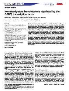
found not to be bound by a TF in ChIP-chip experiments (typically these are the genes with highest p-values and thus least significant binding). A schematic representation of the classification workflow is presented in Figure 1. See the Methods section for a full description of classifier construction and validation. Using several genomic datasets (described below) an SVM classifier is constructed for each TF on a chosen set of features and then evaluated using a leave-one-out cross validation approach. Some difficulties remain for choosing the negative set at this stage. The selection of negatives does not guarantee that the chosen genes are truly not targets of the TF. In the worst cases where some TFs have few known targets, the classifier would contain only a few negative examples. This can introduce fluctuations in the results, biasing the performance in unpredictable ways. Under-sample negative set

Training Set

Feature Reduction and Classifier Construction •SVM-RFE to select top 1500 features.

genes

features

leave-one-out cross validation loop

Final Training Classifie r

•Train Platt’s SVM on selected features.

Single Accuracy Estimate

evaluate on test set Testing Set

Testing Set

Repeat validation with new resampling of negatives. Average the Accuracy estimates over 100 repeats.

100X Average Accuracy

Figure 1 - SVM Framework This figure shows the data mining scheme for making TF classifiers. 100 classifiers are constructed for each TF, each using a different random sub-sample of the negative set. First, on the far left, the negative pool for a TF is under-sampled, so that it is the same size as the positive set. A classifier built on the training set is evaluated using leave-one-out cross validation (center, dashed box). For every cross-validation split, the top 1500 features are selected using SVM-RFE and the classifier is trained and finally used to classify the test set (left out sample). This process is repeated 100 times, and the accuracy for the procedure is the average of the 100 cross-validation accuracies. To classify a potential new target for a TF, all 100 classifiers are applied to the gene’s feature vector, and the average posterior probability is calculated (probability of being a target). A probability greater than 0.5 indicates a positive classification.

To resolve these difficulties we first assure that the pool of possible negatives is a minimum of 600 genes, or at least three times the size of the positive set. From this pool we randomly select a set of negatives which is equal in size to the known positives. After constructing and validating a classifier on these examples, the process is repeated one hundred times, each time with a new random resampling from the -

-5--

negative pool. The average cross-validation accuracy from all repeats is reported. This assures that small-sample classifiers are challenged with a diverse set of negatives and that fluctuations due to errors in the negative set tend to average out. Once the choices of positive and negative sets are made, genes are described by a set of attributes or features to be used by the algorithm to learn the classification rule. A gene may be described by its expression measurements over a set of conditions, or perhaps by counts of various motifs present in its promoter. For example, to capture the sequence composition of a gene’s promoter, all possible nucleotide patterns of length 4 may be counted in the 800 base pairs 5' of the transcription start site. This results in a vector 256 elements long, each entry being the count of a particular 4-mer in the promoter. In our previous study, we examined 26 different types of features including various types of k-mer counts, expression data, and phylogenetic profiles. Here we choose 8 feature types selected to represent a diverse set of data including sequence, structure, expression, and conservation. Several things set our current work apart. First, balanced training sets (equal numbers of positive and negatives) and the random resampling of negatives provides for more robust classifiers. Second, rather than using all features to make a classifier we apply recursive feature elimination to select those that are most relevant. Most importantly, a ranking is also created which can be used to identify the specific features that are most useful for separating target genes from non-targets. The simultaneous ranking of all features allows us to easily discover important biological aspects of regulation. Third, several of our methods have been improved. We introduce a new dataset of k-mer counts weighted by their conservation in alignments with sequences from closely related species. Finally, we expand the transcriptional network to include 59 new TFs (163 total) and analyze the global network properties of the regulatory interactions in yeast. This analysis highlights the transcriptional network hubs; the factors which control the most genes and the genes which are bound by the largest set of regulators. Again, Swi6 is taken as an example and a new potential feed-forward loop is discussed which may take part in the cell cycle and DNA damage response.

Results and Discussion Parameter tuning, feature selection, and training set size

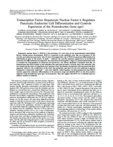
Two parameters must be set in our framework before building a classifier. One parameter, denoted by C, determines the amount of misclassification that is tolerated. The second is the number of features to select during training. Since it would be computationally prohibitive to choose these parameters during the training of every classifier, they are first optimized on the classifier for one TF. The learned values are then applied to the remaining classifiers. The transcription factor YIR018W is chosen for parameter selection since it is known to regulate ~70 genes, which is close to the average for all TFs being analyzed. Features for all genomic datasets are concatenated to produce large attribute sets for each gene. SVM-RFE is used to rank each feature during classifier training (see Methods) and various feature subset sizes are tested using a leave-one-out cross validation. Thus we allow the datasets to adjust, automatically selecting the most important features, irrespective of the data sets from which they originated. Figure 2 shows the effect that changes in feature number have on classifier accuracy. Although as few as five features achieve 70% accuracy, the addition of more features

-

-6--

continues to improve accuracy until 1500 features are selected, where accuracy is approximately 85%. 1500 is then the number chosen for the remaining TFs.

Figure 2 - Feature Elimination YIR018W was used as a prototype to determine the number of features needed to build a classifier. This graph shows the accuracy of classifiers for YIR018W built using different numbers of features selected using SVM-RFE. Error-bars show one standard deviation of 50 classifiers constructed at each feature number using different sub-sampling of the negative set. 1500 features were selected as the point where accuracy reaches a plateau.

Using a grid search as described in Methods, we have chosen C = 0.0078, although results are relatively insensitive to changes in value for C < 1. Classifiers are then constructed for the remaining transcription factors. As discussed in Methods, performance is measured using leave-one-out cross-validation. Since 100 classifiers are trained for each TF using 100 randomly chosen negative sets, the reported accuracy is the average for 100 trials. The accuracy for all yeast binding sites (over all classifiers) is 76%; for the best 25 classifiers it is 86%. All predictions are in the form of a class conditional probability as described in [19]. New predictions are the result of averaging the assigned probabilities from each of the 100 classifiers for a TF. An average probability greater than 0.5 indicates a positive classification. Higher confidence predictions can be obtained by increasing the threshold. Throughout this manuscript probabilities given with the capital P refer to the mean posterior probability assigned by the SVM classifiers (see Methods). Lower-case p refers to pvalues assigned using other statistical tests. Classifier accuracy is loosely correlated with the size of the positive set, where TFs with more known targets tend to have more accurate classifiers (Supplementary Figure 1). This implies that classifier performance could improve in the future, as more experimental targets are discovered. This effect is seen mainly for classifiers

-

-7--

with few positives. Indeed, many classifiers with 20 or fewer positive examples perform poorly. Web Server, Network Visualization and Analysis

One of the origins of network structure is combinatorial regulation; i.e. single TFs often regulate more than one target, and particular targets are often regulated by more than one TF. Such networks can be augmented with data on protein-protein interactions and displayed as a repertoire of connections (the cell’s network repertoire), different subsets of which are selected by particular environments. Here we display the underlying repertoire using the VisAnt analysis and visualization system [1, 2]. The repertoire is available at the VisAnt website and can be accessed in the methods table as “TFSVM.” Visualization in VisAnt allows comparison of predictions to be integrated with many other large scale genomic datasets including protein-protein interaction, gene expression, GO functional annotation, and genetic interaction. VisAnt also includes a sliding bar which allows adjustment of the network based on a threshold for accepting a predicted association. Thus predictions can be embedded in networks mined at any specified degree of stringency for further analysis.

Rfx1 phylogenetic profile predicted functional similarity affinity chromatography yeast-2-hybrid co-purification biophysical interaction

a.

protein

Swi6

known

new

DNA

Rfx1

Rfx1 new

YMR279C

Figure 3 - Partial Regulatory Network of Swi6 A sub-network showing some of the new predictions for Swi6 and how they are interconnected to previously known targets, using the VisAnt browser. Rfx1 and YMR279C are underlined in the network. 3a shows and up-close schematic of the feed-forward loop between Swi6, Rfx1, and YMR279C.

Figure 3 displays a sub-network of known and newly predicted (P > 0.95) targets of Swi6. Only a portion of the known Swi6 targets are shown. This subset was chosen

-

-8--

because the genes are as interlinked with each other as they are with newly predicted targets. The new predictions are highly connected to known targets by a variety of experimental and computational methods, including phylogenetic profiling, genetic interaction, yeast two-hybrid, Bayesian predicted functional similarity, copurification, affinity chromatography, and synthetic-lethal experiments. Both gene groups in Figure 3 contain cell cycle genes, and the most common connection is phylogenetic profiling, suggesting considerable functional similarity. The network perspective supports the prediction of common regulation of these highly interacting genes, and makes it easier to formulate testable hypothesis about the relationships of regulatory targets. It is clear from Figure 3 that a new target of Swi6, YLR176C(Rfx1), is a transcription factor which regulates a previously known Swi6 target, YMR279C. This arrangement is a feed forward loop, suggesting that YMR279C is under strict combinatorial control by these two factors (Figure 3a). It should be noted that although our method independently predicts that Rfx1 is a regulator of YMR279C. Rfx1 was reported to bind the promoter of YMR279C in an early ChIP-chip study[20]. An updated analysis of those results by the same group removed YMR279C from the dataset (can be downloaded from [21]), and a subsequent ChIPchip experiment did not show significant regulation[22]. Due to this ambiguity the Rfx1-YMR279C interaction is not in our positive set; nonetheless, it is predicted by the classifier for Rfx1. Rfx1 is a repressor known to be involved in the cell-cycle DNA damage checkpoint. Inactivation of Rfx1 in response to cellular DNA damage or replication block causes the induction (i.e., de-repression) of many genes[23]. As further evidence that Rfx1 is indeed regulated by Swi6, expression of the two transcription factors was examined during the alpha-factor arrested cell cycle time course[24]. Figure 4 shows the expression of Swi6, Rfx1, and two reference genes which show expression peaks in G1 and S-phase. Across the 18 experiments in the time course, the two factors show a correlation coefficient of 0.6.

-

-9--

Figure 4 - Swi6 and Rfx1 in the Cell Cycle This graph shows the Log2 expression values of Swi6 and a newly predicted target, Rfx1 (also a TF) during the cell cycle. G1 and S-Phase are marked by the expression of two prototype genes, YPL256C and YDR224C, which are known to have peak expression in G1 and S-phase, respectively. Swi6 and Rfx1 show correlated expression during the cell cycle.

Since Swi6 is known to be important for the G1/S transition, the expression in these specific experiments was examined more closely. Using prototypical G1 and S phase reference genes, eight time points spanning the peak of G1 through the peak of S phase were selected. In these eight experiments Swi6 and Rfx1 show a stronger correlation of 0.73, which is statistically significant at p = 0.02. Interestingly, Swi6 binds several genes in the DNA damage response pathway including Dun1(known), Rad53(new, P = 0.96), and Mec1(new, P = 0.76). These targets are upstream kinases known to phosphorylate Rfx1 in the DNA damage response pathway[23]. Finally, it has been shown that Rad53 directly phosphorylates Swi6, delaying progression of the cell cycle into S-phase[25]. The ultimate target of the new feed foreword loop is YMR279C, which is an uncharacterized gene showing sequence similarity to membrane transport proteins. This gene shows a 9-fold induction in response to DNA damage[26]. Taken together, this evidence suggests that Swi6 is crucial to the DNA damage response at the end of G1, and that YMR279C plays a role in DNA damage response and perhaps cell cycle progression. Deletion mutants of YMR279C are viable[27] but it is not known how this deletion affects the cell cycle or DNA damage response. Examining these mutants for deficiencies in growth and DNA damage response may shed some light on the true function of YMR279C. Detailed experiments including reporter assays would be needed to determine how closely interlinked Swi6, Rfx1, and YMR279C are on the transcriptional level. As a working hypothesis, it appears that Swi6 is available to activate DNA damage response genes such as Rfx1, ensuring they are present at crucial times in the cell cycle. Normally Rfx1 is repressing its targets and YMR279C will not be activated. In times of DNA damage Rfx1 is inactivated by a phosphorylation cascade allowing YMR279C and other response genes to be induced by Swi6, resulting in cell cycle arrest. In any regulatory network it is of interest to know which genes are most heavily under transcriptional control, and which TFs exert the most control by regulating large numbers of genes. When analyzing global network properties, we limit our analysis to high quality predictions by only including TFs that have a classification accuracy greater than 0.6 (there are 130 such TFs), and targets that have a true positive probability ≥ 0.95. In the resulting network, many genes are under strong regulatory control. For instance, 125 genes are regulated by 12 or more transcription factors. These genes show statistical enrichment (p ≤ 0.05) in several GO biological process categories. The enriched categories are mainly involved in carbon metabolism and energy generation (see Supplementary Table 1), which are crucial functions expected to be under intense control. Other important processes include DNA damage checkpoint, DNA recombination, DNA damage response, acetyl-CoA catabolism, NADP(H) metabolism, and telomere maintenance. In all, 13 transcription factors show very broad regulatory control. These 13 TFs regulate more than 300 genes each at high significance levels (P≥ 0.95). This set of TFs includes the pervasive regulators Abf1 and Reb1, as well as TFs involved in the cell cycle, growth, and stress response (see Supplementary Table 2). The full set of predictions for 163 TFs in S. cerevisiae are available at http://cagt10.bu.edu/TFSVM/Main%20Frame%20Page.htm . Users may query a -

- 10 - -

transcription factor, returning the list of predicted targets, or a gene, returning a list of possible regulators. The class conditional probabilities described above may also be set by the user, providing an adjustable threshold on the confidence of predictions for each TF. In addition, the cross validated accuracies for all classifiers have been posted online, as well as the top 50 ranked features for each TF-classifier. Prediction Analysis and Feature Rank

As described in Methods, the features for each classifier are ranked using SVM-RFE. Ranked features can be used to reveal interesting biological aspects of regulation and suggest directions for future experiments. We again use Swi6 for a case study. Swi6 interacts with Mbp1 and Swi4 during the cell cycle (G1/S transition) and in meiosis [28, 29]. This TF has 142 known targets and its SVM classifier has a prediction accuracy of 83%. The known targets of Swi6 and the new predictions (at true positive probability thresholds of P > 0.5 through P > 0.95) are significantly enriched (p < 0.05) in the expected GO biological processes including cell cycle, regulation of cell cycle, mitotic cell cycle, DNA repair, etc. Some of the new categories for which targets at P > 0.95 show enrichment include chromatin assembly/disassembly (p = 1e-10), septin checkpoint (p = 2.7e-3), and lipid metabolism (p=8.4e-4). These new targets fit with the current intuition about Swi6 regulation and suggest possible new roles of action. Further regulatory implications can be seen by examining the importance of the features used for classification. Since feature ranking is performed on every training set during cross validation, and because the cross validation is repeated 100 times with random negative sets, there is a total of 14200 feature rankings available (142 examples times 100 cross validation repetitions = 14200 rankings). Using this ensemble of rankings, features are re-ranked based on the frequency with which they appear in the top 40 rank-ordered features. This allows the selection of attributes that are robust to changes in training data and can serve as reliable markers for differentiating regulatory targets. Figure 5 shows a plot of the features for Swi6 sorted by their occurrence in the top 40 ranked features within the 14200 rankings. Only a relatively small number of features retain high importance across a majority of the rankings. The first 10 features are in the top 40 of more than 65% of the rankings while the remaining features fall off sharply in reliability.

-

- 11 - -

Figure 5 - Swi6 Feature Ranking A feature ranking is created on every training set during cross validation of a classifier. Since 100 classifiers are made for every TF, this results in hundreds of separate rankings (100 * #Training Points). This plot shows the frequency with which a feature shows up in the group of top 40 features. When sorted by this frequency, only the most important features remain at the top of the list. For Swi6 the first 10 features are in the top 40 of 60% of the rankings.

The most important feature for identifying known targets of Swi6 is a microarray experiment measuring expression of genes in an Mbp1 deletion mutant. This makes sense since Swi6/Mbp1 interact and function as coactivators at many promoters. By t-test the observed expression change is significant between the negative set and the known positives (p = 3.7e-25), and between the negative set and the predictions made at 95% confidence (p = 9.14e-27, 280 genes). For more details on how microarray data are incorporated as features in the datasets see Methods. The next 4 highest ranked features identify the k-mer ACGCG/CGCGT as being important for classification by conservation and overrepresentation. The k-mer overlaps highly with known binding sites for Swi6; for example, Swi6 binds CGCGAAA in the Cln2 promoter[30]. The overrepresentation of this sequence in the positive training set can be seen by examining the calculated E-values, which are the scores used to determine the significance of each k-mer (see Methods). Viewing this score in the negative set genes as compared to the positives is informative, and Figure 6 plots the distribution of E-values in the genes of the negative set, positive set, and the predicted targets at P > 0.95. The graph was generated by placing the genes in each set (i.e., positive, negative, and predicted) into 5 equally spaced bins based on Evalue. The known and predicted targets clearly show enrichment of ACGCG as compared to the negative genes.

-

- 12 - -

Figure 6 - Overrepresentation of ACGCG in Swi6 Target Promoters This plots the number of genes versus the E-value of ACGCG in groups of target promoters. Three categories of promoters are shown: (i) negative set promoters in blue, (ii) positive set promoters in violet, (iii) predicted targets at P ≥ 0.95. For each category, genes are grouped into 5 equally spaced bins based on the E-value of overrepresentation of ACGCG. The center locations of those bins are plotted on the x axis and the number of genes in each bin is on the y axis. Positive and predicted target promoters of Swi6 show higher overrepresentation of ACGCG than negative set genes.

The conservation of ACGCG is ranked more highly than overrepresentation, indicating that this sequence is preserved in promoter alignments which include 7 Saccharomyces species. Figure 7a shows such an alignment in the promoter region of the Isc1 gene, a newly predicted target of Swi6 (Figure 7b shows a similar alignment in the Sur2 promoter). Two occurrences (highlighted in red) of the indicated k-mer appear in close proximity in a highly conserved segment of the Isc1 promoter. Isc1 is an important gene since it is the only member of the extended family of sphingomyelinases (SMases) which is present in the yeast genome. This SMases are responsible for generating ceramides, which are bioactive lipids known to modulate a variety of cellular processes including cell growth, senescence, apoptosis, and the cell cycle[31]. They also contain a newly discovered P-loop-like domain, which is conserved in the SMase family from yeast to humans[32]. Isc1 is the closest yeast homolog to the human neutral SMase2 gene and has thus become the prototype for exploring the functions of this enzyme class.

-

- 13 - -

a

Conservation

start

S. cerevisiae S. paradoxus S. mikatae S. kudriavzevii S. bayanus S. castelli S. kluyveri SVM conserved pattern: ACGCG/CGCGT in the promoter of ISC1 Transcription factor SWI6 (YLR182W)

Figure 7 - Conservation of ACGCG in Swi6 Target Promoters This figure shows multi-genome alignments of selected promoter regions of Swi6 targets taken from the USC Genome Browser. Instances of ACGCG and its reverse complement are highlighted in red. The conservation score is the output of the PhastCons algorithm. The score is a posterior probability assigned to each nucleotide, giving the likelihood that the nucleotide resides in a conserved element, as defined by a hidden Markov model of “slow” and “fast” evolution. A) alignment in the promoter region of ISC1, showing two instances of the ACGCG motif. B) alignment in the promoter region of Sur2, also showing two instances of the conserved motif.

Isc1 is a new prediction, not previously annotated as a target of Swi6. The regulation of Isc1 is now being actively explored, and it was recently shown that Isc1 is linked to cell growth in yeast[31] as well as being important for fermentative growth and sexual reproduction[33]. Perhaps more importantly, recent experiments in human and mouse models have demonstrated ceremide enhanced cancer cell death, indicating that ceramide could act synergistically with other chemotherapeutic agents[34]. Indeed, several therapeutic compounds are currently under development which modulate ceramide metabolism. The prediction that Isc1 is regulated by Swi6(Mbp1) is significant since it provides a direct link between cell cycle regulation and the generation of bioactive lipids via the hydrolytic pathway. Further investigation will be necessary to determine the biological significance of this link and whether the human ortholog, SMase2, shows a similar connection to the cell cycle. It is possible that ceramide production via SMase2 could serve as a target for anti-cancer therapy which can be easily studied in yeast models. It would be of interest to create sphingomyelinase inhibitors which would help in dissecting the specific roles of the ceramide biosynthetic pathway (SMase independent) and the hydrolytic pathway (SMase dependent) in regulating ceramide levels and cell death. The information that predicted targets of Swi6 include SMase and are enriched in genes functioning in cellular lipid metabolism (GO category p-value=8.4e-4) suggests that Swi6 has a greater role than previously appreciated in controlling lipid metabolism and its coupling to cell growth, apoptosis, and reproduction. -

- 14 - -

As a further example of the usefulness of SVMs coupled to a robust feature ranking, we briefly explore the results for the TFs Gzf3 (YJL110C), and Ash1 (YKL185W). The feature ranking for the factor Gzf3 (YJL110C) indicates that the melting temperature at positions -274 to -286 in target promoter regions is different than that in non-target promoters. Figure 8 shows a plot of the average melting temperature in sets of yeast promoters averaged within a moving 20bp window. Known targets clearly have a reduced melting temperature at the identified positions as compared to negative set or average genes. The relationship is still present in the targets which show a true-positive probability >0.95. This group contains 72 targets, 27 of which are new predictions. Although it is unclear how the melting temperature and helix stability in this region affects regulation by Gzf3, it is possible that Gzf3 or other factors induce changes in DNA compaction or stability which alter regulation at these promoters. Binding sites of Gzf3 do not appear to be concentrated in this region, implicating the activity of other factors at this site. In any case, feature ranking has identified specific nucleotides which can be tested experimentally for their role in transcriptional regulation.

Figure 8 - YJL110C Target Melting Temperature Plot Using a 20bp window for DNA melting temperature calculation, temperature plots are presented for the average over all 5571 yeast genes (solid blue), positive targets for YJL110C (dashed red), negatives for YJL110C (dashed blue), and high confidence targets (solid red—P(true|distance to separator) ≥ 0.95) determined using Platt’s method for probability assignment to SVM output. Targets of YJL110C have a lower melting temperature than the average or negative set gene. SVM feature ranking correctly identifies the window positions in which the target melting temperature is most unlike that for negative genes, suggesting altered promoter structure of the targets, which is conserved at positions -286 to 274.

The classifier for Ash1 has a prediction accuracy of 88%. The highest ranked feature is expression in She4 deletion mutants. Expression of known targets and new predictions is significantly different than in the negative set (p=5.4e-15 and p=6.5e-8

-

- 15 - -

respectively). Ash1 mRNA is localized to the daughter cell late in the cell cycle, where it prevents mating type switching by repressing HO genes[35, 36]. Localization of Ash1 mRNA is dependent on She genes. Specifically She4 binds to the myosin motor protein She1, and deletion of She4 causes loss of actin polarization[35, 37]. Thus, deletion of She4 prevents appropriate localization and regulation by Ash1, resulting in the observed increased expression of Ash1 target genes.

Conclusions Transcription factor binding site prediction is a difficult problem in computational biology. Our SVM-based approach generates classifiers for each TF, and the reliability of the predictors is assessed using cross validation. The selection of high confidence predictions is made simpler by the calculation of a posterior probability for each potential target gene. By incorporating many types of genomewide measurements into a robust feature ranking system, it is possible to discover important biological aspects of regulation which are specific to each TF being studied. This has been demonstrated on the yeast cell cycle regulator, Swi6. The predicted targets of Swi6 match the known biology of the regulator and suggest possible new roles of action in bioactive lipid metabolism and the DNA damage response. Moreover, feature ranking has identified interesting biological properties of the regulator including expression change of its targets in Mbp1 deletion mutants, and over-representation/conservation of the motif ACGCG. Similar analyses can be carried out with other TFs, as shown with Gzf3 and Ash1, for which meaningful biological features are identified. Investigators may download predictions made for all TFs, view classifier accuracies, and download lists of top-ranked features for each regulator at the provided web server. Custom analyses of the full yeast transcriptional network can also be accessed online in the VisAnt browser. The next step of this analysis is to apply these methods to the human genome and assess their reliability. The possibility exists for the development of an electronic-chip-ChIP in human genome, whereby thousands of predictions can be made and the most reliable of these can be tested experimentally.

Methods SVM training and validation

The SVM is a statistical learning method originally developed by Vapnik [38]. SVMs are based on rigorous statistical principles and show excellent performance when making predictions on many types of large genomic datasets. The algorithm seeks a maximal separation between two groups of binary labeled (e.g., 0, 1 or negative, positive) training examples [39]. The training examples are feature vectors x of individual genes, each vector populated by measurements taken on genome scale datasets (see below). These measurements are the attributes of the data. A single classifier based on these features is then constructed to predict targets for each TF. Positives are genes which are known targets of the TF, and negatives are a randomly chosen subset of genes (equal in size to the positive set) which are least likely to be targets. The separation of targets from non-targets is accomplished by an optimization which finds a hyperplane separating the two classes. The hyperplane is chosen to be as distant as possible from the data points, thus creating a maximalmargin hyperplane. The classifier can then be applied to new, unlabeled genes. We

-

- 16 - -

have successfully applied SVMs to regulatory predictions before[17, 18, 40], and an in-depth tutorial on SVM training is available on our website. The C parameter must be specified in SVM training. This parameter adjusts the tolerance of the algorithm for misclassifications. As with feature selection (described below), the classifier for YIR018W was used as the prototype for parameter selection. Grid selection was performed on the training set for YIR018W using many values of C, and classifier accuracy was measured with 5-fold cross validation. The SVM was seen to be insensitive to the choice of C, with most values less than 1 showing similar performance. Tested values include: [2-7 2-5 2-3 2-1 1 1.5 2 22 23 24 25 26]. The value 0.0078 was chosen as this was the value reported by the SPIDER machine learning package[41] as having the best performance. Choosing negatives for TF target prediction can be difficult, since there is no defined set of genes known not to be targets. As in our previous work, ChIP-chip results can serve as a guide. For every TF, ChIP-chip results are used to identify genes which have the highest p-values (least significant) for binding under all tested conditions. The number of negatives is chosen to be at least three times the size of the positive set, or at least 600 genes, whichever is larger. Classifiers constructed on different randomly chosen negatives may give different results, since some unknown targets may be incorrectly assigned to the negative set. To smooth out these fluctuations, 100 classifiers are constructed for each transcription factor using a random resampling from the negative set. Each resampling is equal in size to the positive set and all 100 classifiers are tested using leave-one-out cross validation (LOOCV). The final performance statistics (accuracy, PPV, etc.) are averages from the 100 trials. The scheme used here for classifier construction is outlined in figure 1. To illustrate the construction and validation more concretely, a short outline is provided below. For an example TF-A: 1. Assemble positive set. Sample n genes randomly from the negative pool (see above) to construct the negative set (n = number of known targets). 2. Spit the data for LOOCV. 3. Use SVM-RFE to rank all features in the training set. 4. Construct SVM classifier on top 1500 features. Save full feature ranking. 5. Classify left out gene. 6. Repeat steps 2-5 to complete LOOCV. Save all feature rankings. 7. Calculate performance statistics (Accuracy, PPV, etc.) 8. Repeat steps 1-7 100 times. 9. Calculate final performance statistics (i.e., mean Accuracy, mean PPV, etc.). A new gene can be classified by applying all 100 classifiers for TF-A to the feature vector for that gene. Each classification produces a posterior probability (see below), and the mean of all 100 probabilities is calculated. If P>0.5, classify the gene as a target of TF-A. The full set of feature rakings on every training set is used to calculate the final feature rank (see below). Classifying new targets and prediction significance

As described in [19], SVMs can provide a probabilistic output which in this case measures the likelihood that any given gene is a target. This is given in the form of a class conditional probability, P(target | SVM output), where “SVM output” is the distance of the gene from the separating hyperplane. These outputs can be referred to as Platt’s posterior probabilities (after the author of [19]) or simply as the true positive probability. The intuition of this method of assigning probabilities is that data points

-

- 17 - -

which are deeper in the positive region (i.e., further from negative examples) are the most likely to be true positives. Our classifiers are trained for probabilistic output as recommended in [19], and new genes are classified using the average probability assigned by all 100 classifiers for a given TF. An average posterior probability greater then 0.5 is considered to yield a positive. Throughout the manuscript we refer to this probabilistic output using the upper-case P (e.g., P>0.99), whereas p-values measured by other means are shown in lower-case (e.g., p