Cache Oblivious Parallelograms in Iterative Stencil Computations Robert Strzodka
Mohammed Shaheen
Dawid Paja¸k
Max Planck Institut Informatik Campus E1 4 Saarbrücken, Germany
Max Planck Institut Informatik Campus E1 4 Saarbrücken, Germany
[email protected]
[email protected]
West Pomeranian University of Technology ˙ Zołnierska 49 Szczecin, Poland
[email protected]
Hans-Peter Seidel Max Planck Institut Informatik Campus E1 4 Saarbrücken, Germany
[email protected] ABSTRACT
1.
We present a new cache oblivious scheme for iterative stencil computations that performs beyond system bandwidth limitations as though gigabytes of data could reside in an enormous on-chip cache. We compare execution times for 2D and 3D spatial domains with up to 128 million double precision elements for constant and variable stencils against hand-optimized naive code and the automatic polyhedral parallelizer and locality optimizer PluTo and demonstrate the clear superiority of our results. The performance benefits stem from a tiling structure that caters for data locality, parallelism and vectorization simultaneously. Rather than tiling the iteration space from inside, we take an exterior approach with a predefined hierarchy, simple regular parallelogram tiles and a locality preserving parallelization. These advantages come at the cost of an irregular work-load distribution but a tightly integrated loadbalancer ensures a high utilization of all resources.
Naive implementations of stencil computations suffer heavily from system bandwidth limitations. Various cache blocking techniques have been developed to optimize for the spatial data locality in this case. Kamil et al. [8] present recent empirical results and Frumkin and van der Wijngaart [5] have tight lower and upper bounds on the number of data loads. However, optimization of a single stencil application remains by construction bounded by the peak system bandwidth. In view of the exponentially growing discrepancy between peak system bandwidth and peak computational performance, this is a severe limitation for all current multicore devices and even more so for future many-core devices. In order to surpass system bandwidth limitations, we must turn to iterative stencil computations and reduce the offchip traffic significantly by exploiting temporal data locality across multiple iterations. Wolf [17], Song et al, [15] and Wonnacott [18] presented the first of the so called time skewing schemes. The idea is to look at the entire iteration space formed by the space and time, the space-time, and divide it into tiles that can be executed quickly in cache. To proceed to the next step locally without access to main memory, stencil computations require the neighbors of the previous iteration, therefore the tiles in the space-time are skewed with respect to the time axis, see Fig. 2. The execution inside the tile is very fast because these values are produced and consumed on-chip without the need for a main memory access. Only at the tile boundaries additional data must be brought into cache. If we know the L2 cache size in our CPU we can choose the tile size such that the base of the tile fits into the cache. To optimize for a memory hierarchy we could further divide the tile into small tiles, whose bases fit into the L1 cache. All such parameters must be set conservatively, because any overestimation leads to cache thrashing and a severe performance penalty. In a multi-threaded environment it is difficult to find the right parameters, since the available cache can be shared by different application threads and it is not clear which portion of the cache is available to the stencil computation at any given time. A scheme that is able to exploit the memory hierarchy without explicitly knowing its sizes is called cache oblivious.
Categories and Subject Descriptors D.1.3 [Programming Techniques]: Concurrent Programming—parallel programming; G.4 [Mathematical Software]: efficiency, parallel and vector implementations
General Terms Algorithms, Design, Performance
Keywords memory wall, memory bound, stencil, time skewing, temporal blocking, cache oblivious, parallelism and locality
Permission to make digital or hard copies of all or part of this work for personal or classroom use is granted without fee provided that copies are not made or distributed for profit or commercial advantage and that copies bear this notice and the full citation on the first page. To copy otherwise, to republish, to post on servers or to redistribute to lists, requires prior specific permission and/or a fee. ICS’10, June 2–4, 2010, Tsukuba, Ibaraki, Japan. Copyright 2010 ACM 978-1-4503-0018-6/10/06 ...$10.00.
INTRODUCTION
Frigo and Strumpen [3] introduced a cache oblivious stencil scheme that divides the iteration space recursively into smaller and smaller space-time tiles and thus generates high temporal locality on all cache levels without knowing its sizes. The cache misses are greatly reduced leading to the desired reduction of system bandwidth requirements, however, the performance gains are relatively small in comparison to this reduction. Strumpen and Frigo [16] report a 2.2x speedup against the naive implementation of a 1D LaxWendroff kernel on a IBM Power5 system for periodic and constant boundary conditions after optimizing the software aspects of the scheme. After multifold optimizations and parameter tuning Kamil et al. [9] achieve a 4.17x speedup on the Power5 (15 GB/s theoretical peak bandwidth), 1.62x on an Itanium2 (6.4 GB/s) and 1.59x on an Opteron (5.2 GB/s) system for a 7-point stencil (two distinct coefficient values) on a 2563 domain for periodic boundary conditions. However, for constant boundary conditions the optimized cache oblivious scheme is only faster on the Opteron achieving a 2x speedup at best. The compared naive code is optimized with ghost cells and compiled with optimization flags. The above optimizations of the cache oblivious scheme are all directed at single-threaded execution. Frigo and Strumpen later analyzed multi-threaded cache oblivious algorithms [4]. One example deals with the cache misses of a 1D stencil code with parallel tile cuts. Blelloch et al. [1] discuss the construction of nested parallel algorithms with low cache complexity in the cache oblivious model for various algorithms including sparse matrix vector multiplication. However, these are mainly theoretical papers and we do not know of any parallel, high performance cache oblivious implementations of stencil computations based on these ideas. A more general approach to improve the temporal locality of iterative stencil computations is to see them as a special case of nested loops with data dependencies. The polyhedral model provides an abstraction for valid transformations of such nested loops. For an automatic source-to-source translation three steps are required: dependence analysis, transformations in the polyhedral model and code generation. Bondhugula et al. [2] present a complete system called PluTo [13] comprising all three steps. Given a source file it generates the optimized transformed code that can be compiled instead of the original source. Obviously, PluTo cannot successfully exploit data dependencies hidden behind complex index or pointer arithmetic, but it performs very well when arrays are allocated statically and data dependencies are expressed clearly. Other state-of-art tiling schemes for nested loops are HiTLoG [7, 10] and PrimeTile [6, 14]. Harton et al. [6] compare the performance of these tools and they do not differ much on the, for us relevant, Gauss-Seidel and FDTD solvers, therefore we will compare only against PluTo in the result section. The contribution of this paper is a new cache oblivious scheme for iterative stencil computations that delivers the high speedups promised by the great cache miss reduction and clearly outperforms more general transformation tools and optimized naive code. We compare the performance also to a synthetic benchmark version of the stencil kernel that operates exclusively on registers with no data transfers. The most impressive results are achieved in 2D when the benchmark iterates over registers (25.1 GFLOPS) and our scheme iterates over a gigabyte large domain (19.1 GFLOPS) and
they lie less than 25% apart, as if system bandwidth hardly mattered at all, see Section 3.1. The next section (Section 2) presents our algorithm in detail. We start with the description of the hand-optimized naive scheme, then explain our cache oblivious approach in multiple sub-sections. Section 3 discusses the results in double precision on 2D and 3D domains. Constant stencils, banded matrices and a FDTD solver are presented. We draw conclusions in Section 4.
2.
CACHE OBLIVIOUS PARALLELOGRAMS (CORALS)
On a discrete d-dimensional domain Ω:= {1, . . . , W1 } × . . . × {1, . . . , Wd } with N := #Ω values we want to apply the stencil S : Ω × {−1, 0, +1}d → R repeatedly to the entire domain T -times. In case of a constant stencil, S does not depend on Ω and has a certain number of non-zero values NS := #S, otherwise we assume that the stencil is position dependent, S(x) : {−1, 0, +1}d → R, x ∈ Ω and has the same number of non-zero values NS for every position, and N · NS values overall. Our space-time domain is given by Ω × {0, . . . , T } with the initial values at Ω × {0} and boundary values at ∂Ω × {0, . . . , T }, ∂Ω:= {0, W1 +1}×. . .×{0, Wd +1}. In the spacetime Ω×{0, . . . , T } there are T N values to be computed, and each output value requires NS input values. So in case of a constant stencil we perform T N NS reads and T N writes; in case of a variable stencil (banded matrix) we perform 2T N NS reads and T N writes. If we access values from timestep t − 1 to compute values at timestep t then irrespective of the scheme, we need to store two copies of Ω during the stencil application. Some stencil computations like Gauss-Seidel, that use values from timestep t − 1 and t while computing timestep t, can be performed in-place with just one copy of Ω. If these one/two copies of Ω fit into the cache, then all reads and writes will happen in the cache no matter how large T is. The naive scheme performs best in this case, as can be seen for 0.5 million elements in the Figs. 10 and 12.
2.1
NaiveSSE Scheme
The naive stencil implementation progresses with the entire domain from Ω × {t − 1} to Ω × {t}, see Fig. 1. Ω is divided into tiles of equal size along one of the spatial dimensions such that each tile is processed by one thread. The threads are synchronized before proceeding to the next timestep with a standard pthreads barrier synchronization. The stencil computation is vectorized with SSE2 intrinsics along the unit stride dimension.
2.2
CORALS Overview
The scheme starts by covering the entire space-time with a single large tile to which we assign all the available threads (Section 2.3). Then we run some preprocessing that generates data for the load-balancer (Section 2.6). The initial tile is divided recursively into a high number of identical base tiles for which we stop the recursion. During the recursion the division tries to distribute the threads and thus assign fewer and fewer threads to the sub-tiles (Section 2.4). The thread distribution is governed by the load balancer (Section 2.6). On each base tile, the kernel containing the actual stencil computation is invoked with a single thread
t
t
111111111111111111111111111111111111111111 000000000000000000000000000000000000000000 000000000000000000000000000000000000000000 111111111111111111111111111111111111111111 000000000000000000000000000000000000000000 111111111111111111111111111111111111111111 000000000000000000000000000000000000000000 111111111111111111111111111111111111111111 000000000000000000000000000000000000000000 111111111111111111111111111111111111111111 000000000000000000000000000000000000000000 111111111111111111111111111111111111111111 000000000000000000000000000000000000000000 111111111111111111111111111111111111111111 000000000000000000000000000000000000000000 111111111111111111111111111111111111111111 000000000000000000000000000000000000000000 111111111111111111111111111111111111111111 000000000000000000000000000000000000000000 111111111111111111111111111111111111111111 000000000000000000000000000000000000000000 111111111111111111111111111111111111111111 000000000000000000000000000000000000000000 111111111111111111111111111111111111111111 000000000000000000000000000000000000000000 111111111111111111111111111111111111111111 000000000000000000000000000000000000000000 111111111111111111111111111111111111111111 000000000000000000000000000000000000000000 111111111111111111111111111111111111111111 000000000000000000000000000000000000000000 111111111111111111111111111111111111111111 000000000000000000000000000000000000000000 111111111111111111111111111111111111111111 000000000000000000000000000000000000000000 111111111111111111111111111111111111111111 000000000000000000000000000000000000000000 111111111111111111111111111111111111111111 000000000000000000000000000000000000000000 111111111111111111111111111111111111111111 000000000000000000000000000000000000000000 111111111111111111111111111111111111111111 000000000000000000000000000000000000000000 111111111111111111111111111111111111111111 000000000000000000000000000000000000000000 111111111111111111111111111111111111111111 000000000000000000000000000000000000000000 111111111111111111111111111111111111111111 000000000000000000000000000000000000000000 111111111111111111111111111111111111111111 000000000000000000000000000000000000000000 111111111111111111111111111111111111111111 000000000000000000000000000000000000000000 111111111111111111111111111111111111111111 000000000000000000000000000000000000000000 111111111111111111111111111111111111111111 000000000000000000000000000000000000000000 111111111111111111111111111111111111111111 000000000000000000000000000000000000000000 111111111111111111111111111111111111111111
15
1
30
4
45
16
60
64
x
Figure 1: Naive space-time traversal. The entire spatial domain executes one timestep after another in sync. The progress of the space-time coverage is shown in color.
even if more threads are still assigned to the base tile. So all parallelization must occur through the thread distribution during the recursive division, the kernel execution itself is single-threaded. In higher dimensional space-time this task is easier (Section 2.5). The choice of the base tile and other internal parameters are discussed in Section 2.7.
2.3
Parallelograms in 2D
As discussed in the introduction, the attempts to extract high absolute performance from the original cache oblivious stencil scheme were not very successful, although cache misses are significantly reduced and hardware specific optimizations were applied. We think that one of the problems lies in the irregularity of the generated space-time tiles, because the compiler and hardware generally perform much better on regular data structures. Therefore, a main design aspect of CORALS has been the preservation of the theoretic asymptotic behavior of the original cache oblivious stencil scheme while utilizing only regular execution patterns: CORALS applies the hierarchical decomposition idea to a single-form space-time tile, namely a parallelogram. The following parallelization and data locality strategies are a consequence of this decision. Parallelograms have a favorable surface area to volume ratio. They have the advantage that we can iterate over the interior points with simple nested loops where each loop always executes the same number of runs, only the bounds are skewed with respect to the time. This allows an efficient vectorized execution with explicit control of data alignment. As we have only a single tile form, only one such specialized kernel must be implemented. Moreover, parallelograms split easily into identical sub-parallelograms and also allow a regular parallelization. As there are only parallelograms in the scheme we start with a large parallelogram that covers the entire space-time, see Fig. 3. This figure shows that an exterior coverage of the domain leads to different work-loads inside the tiles. Section 2.6 on load-balancing discusses this in detail. In the following let us assume that we deal with parallelograms
x
Figure 2: Hierarchical, cache oblivious space-time traversal. Different parts of the spatial domain progress in time at different speeds. Only at the end the entire spatial domain reaches the same timestep. The progress of the space-time coverage is shown in color. that lie completely inside the space-time. Fig. 4 shows the canonical subdivision scheme for the parallelogram. The dimensions of the initial parallelogram are made divisible by a large power of two, such that we can perform correspondingly many subdivisions without having to half an odd number. Consequently the sub-parallelograms are identical in shape. The figure also shows the thread distribution for an interior parallelogram. The upper left and lower right sub-parallelograms are independent of each other, so given n threads, each of them is assigned n/2 threads and they are executed in parallel. Frigo and Strumpen suggest a spatial trapezoid parallelization in their multithreaded cache oblivious 1D stencil algorithm [4] and this is also the usual choice in cache aware time skewing schemes, but 2D parallelograms are not suitable for that. The spatiotemporal parallelization is a simple solution to this problem.
2.4
Parallelism and Locality
In Fig. 4 two of the four sub-parallelograms are executed in parallel, so in case of n = 2 threads the overall execution time would be reduced to 34 rather than 12 . However, the cache oblivious scheme performs a recursive subdivision of the tiles, so wherever we have more than one thread per sub-parallelogram, it is further divided in the same fashion. Fig. 5 shows the thread distribution after three division steps in case of n = 2 threads. We see that almost the entire domain is parallelized and only the small blocks on the diagonal still require further division for parallelization. After a few division steps the reduction of the overall execution time converges quickly to 12 according to a geometric series. Let us formalize the above reasoning for two threads at first considering the effects of parallelism only. All parallelization must be made explicit through subdivision, so the processing of an undivided parallelogram takes the same time no matter how many threads are assigned to it. Let the initial undivided parallelogram have base width w and height h then its execution time is wh in an appropriate time unit. After the first division, two of the sub-parallelograms run in parallel so the overall time is 34 wh = 12 (wh/2 +
t
n threads
n/2 threads
n/2 threads
n threads
Space time
x
Figure 3: The entire space-time covered by a large initial parallelogram. The work-load on the subparallelograms is substantially different.
2
1 1
1
2
1
1
1
2
2
2
1 1 2
1
2 1
2 1
2
4 2
4 4
4
2
1
1
2 1
2
2
1
2
1
1 1
2
1
1
2
1
2 2
Figure 4: The thread distribution for a 2D cut of an interior parallelogram. The upper left and lower right sub-parallelograms are independent and run in parallel.
2 1
2 1
4
1
2
2
4
2
1
1 1
2
2
1
4
1
2
2 1
1 2
1
Figure 5: Recursive application of the 2D subdivision from Fig. 4 in case of two threads. Subparallelogram assigned with one thread execute in parallel with another sub-parallelogram. wh), where 12 (wh/2) corresponds to the sub-parallelograms with one thread assigned and 12 wh corresponds to the two sub-parallelograms with two threads assigned, see Fig. 4. In the next step each of the two sub-parallelograms with two threads assigned undergoes the same parallelization as the initial parallelogram so the 21 wh is replaced by 34 ( 12 wh) or equivalently wh is replaced by 43 wh as before, giving 1 (wh/2 + 12 (wh/2 + wh)) overall. The following division 2 replaces the last wh in the same fashion and we obtain a recursive formula for the execution time in dependence on the division depth:
execT(0)
= wh 1 execT(1) = (wh/2 + wh) 2 1 1 execT(2) = (wh/2 + (wh/2 + wh)) 2 2 1 1 1 execT(a) = (wh/2 + (wh/2 + (. . . ))) 2 2 2 „ « 1 1 1 = wh/2 + . . . + ( )a + 2( )a 2 2 2
4
2
2
1
2
1
Figure 6: Recursive application of the 2D subdivision from Fig. 4 in case of four threads. Dotted lines show the additional subdivisions in comparison to two threads from Fig. 5. „ « 1 = wh/2 1 + ( )a . 2
(1)
For two threads the geometric series converges quickly to the ideal execution time reduction by 21 . In cache aware time skewing schemes, flat parallelization strategies are applied [11,12,18]. The cache sizes are known, so it is clear when it is better to parallelize the execution of the sub-tiles, forcing them into different caches, and when to leave them in the same cache for better data locality and process them sequentially with a single thread. In the cache oblivious case we do not have this information so on the one hand we must ensure that the parallelism really speeds up the computation, as demonstrated above, and on the other hand we must maximize the tile sizes that are processed by a single thread for best data locality within the same cache (we assume the scalable scenario where caches are not shared between cores). A similar reasoning as above shows that the second condition is also fulfilled. The first division assigns already half of the domain to the local execution by a single thread, the next division adds a half of the remaining half leading to a geometric series again 12 + 14 +. . .. At some stage the tile bases are smaller than the cache so the parallelization will force its sub-tiles into different caches destroying the
data locality between the sub-tiles, but this happens only in a small part of the domain that correspond to the trailing end of the above series. In conclusion, the scheme preserves as much data locality as possible while converging to the full parallel speedup according to a geometric series. The parallelization in case of more threads is not much different. Fig. 6 shows how the division simply continues in all parts of the domain as long as more than one thread is assigned to a parallelogram. If we stop the recursion at a certain level then we are left with one diagonal of small parallelograms where still four threads are assigned and multiple thin sub-diagonals of parallelograms where still two threads are assigned. This only adds more trailing factors in addition to the already existing ( 21 )a in formula (1), so the properties of the geometric convergence to the full speedup of 4x in case of four threads remains unchanged. The geometric convergence property also holds for an arbitrary number of threads but we cannot expect perfect strong scaling with the thread count because the more threads there are the more divisions are necessary to arrive at the local single thread execution of a tile. However, for weak scaling the domain would also grow, increasing the number of divisions before we reach a fixed base parallelogram size, just as required above. All parallelograms in Figs. 5 and 6 that have been assigned a single thread are also further divided for the cache oblivious data locality but no more parallelism needs to be extracted in these divisions. These division are not included in the figures to facilitate the reasoning about the generated parallelism. Ultimately the entire initial parallelogram is divided into a large number of identical base parallelogram on which we stop the recursion and call the kernel with the stencil computation.
2.5
Parallelograms in mD
This section explains our scheme for an arbitrary dimension m of the space-time. We explain the differences to the 2D iteration space and refer for analogy to the previous 2D figures. In an m-dimensional space-time we have m − 1 spatial dimensions formed by a tensor product of the individual spatial dimensions. The space-time tiles in 2D are parallelograms, in 3D parallelepipeds and in general m-parallelotopes in mD. The projection of an m-parallelotope onto the time axis and one of the spatial axis always gives a parallelogram as depicted in Fig. 3. So all the spatial dimensions are skewed with respect to time and in analogy to 2D we can create an m-parallelotope large enough to cover the entire space-time, see Fig. 3. For the properties of the recursive division and the parallelization, the skewing and the absolute sizes of the different tile dimensions play no role, so instead of an m-parallelotope one can also think of a simple m-hypercube in the following, where all cuts are axis aligned. Fig. 4 shows a 2D division into 22 = 4 sub-parallograms. With a single cut we could also make a 1D division in 2D delivering 21 = 2 identical sub-parallelograms. The m-parallelotope allows kD cuts with k = 1, . . . , m. A kD cut of the m-parallelotope gives 2k identical sub-parallelotopes. The number of created subparallelotopes and their following parallelization does not depend on the space-time dimension m but on the cut dimension k. The reason for considering cuts of different dimensions is that depending on the parameter settings we
want to stop cutting one dimension at a certain tile size, e.g. the unit stride dimension, while other dimension should still be cut. This leads to the applications of different cuts during the recursive division of tiles. The parallelization of the 2D cut requires 2 + 1 = 3 execution stages (with synchronization in between) with the following sub-parallelograms in each ` ´number ` of ´ independent ` ´ stage: 20 = 1, 21 = 2, 22 = 1, cf. Fig. 4. Similarly, for a kD cut we have k + 1 stages where the series ` ´ of independent sub-parallelotopes in each stage is: kj , j = 0, . . . , k. So with higher dimensional cuts, it is much easier to extract parallelism from the division scheme, e.g. a 4D cut (applicable to 3D spatial domains and higher) gives a series of 1, 4, 6, 4, 1, i.e. after finishing the first sub-parallelotope there are already four independent sub-parallelotopes that can be executed in parallel. In mD space-time it is also possible to extract purely spatially independent sub-tiles. The independence of the upper left and the lower right parallelogram in Fig. 4 is spatiotemporal. But if the time dimension is very small, e.g. only T = 10 iterations of the stencil computation are required, then we do not want to cut it further, and a spatial 1D cut would only generate two dependent tiles with no opportunity for parallelism. However, in mD space-time with m > 2, simultaneously cutting multiple spatial dimensions produces spatially independent sub-tiles even if the time dimension is uncut. The better parallelization potential of higher dimensional cuts means that in the recursive division we can more quickly distribute threads and need less depth to reach the local single thread execution on a tile. Figs. 5 and 6 depict the recursive division with 2D cuts. With higher dimensional cuts, the size of the tiles that still need further division decreases faster and thus the geometric convergence (formula (1)) to the full speedup is also faster.
2.6
Load-Balancer
The thread distribution from Fig. 4 assumes that the parallelized execution of the upper left and the lower right subparallelogram have the same work-load, so assigned with the same number of threads, they will finish at approximately the same time without creating idle time at the following synchronization point. Because of our exterior structure (Fig. 3) many parallelograms do not have the same workloads and this results in some idle time at the synchronization points. The CORALS scheme is fast even with this handicap. This section describes the further performance enhancement of the load-balancer. The load-balancer distributes the threads to the parallelized sub-parallelogram according to the actual work-load. To determine the work-load, we execute a preprocessing step that determines the number of interior points for the entire parallelogram hierarchy. This preprocessing uses the same recursive division only with a simpler thread distribution scheme (Fig. 7), because no sub-tile dependencies have to be observed here. The interior points are counted on the base tiles and summed up recursively on the way up, see Alg. 1 on the left. During the actual stencil computation (Alg. 1 on the right) the numbers of the interior points of the independent subparallelograms are put in relation to their sum and the available threads are distributed according to these ratios. Currently, we use a simple distribution model balancing pairs of
n/4 threads
n/4 threads
n/4 threads
Figure 7: The thread distribution for a 2D cut during the preprocessing, see Alg. 1 on the left. No sub-parallelogram dependencies need to be respected here.
n threads
n 01 threads
n/4 threads
n threads
n 10 threads
Figure 8: The thread distribution for a 2D cut during the stencil computation with the load-balancer, see Alg. 1 on the right. Usually we have n01 +n10 = n and the corresponding two sub-parallelograms execute in parallel.
Algorithm 1 The CORALS preprocessing and stencil computation. Both functions take the same recursive descend through the sub-tiles only the parallelization is different. The preprocessing evenly distributes the current thread range onto the sub-tiles without explicit synchronization (Fig. 7), whereas the stencil computation distributes the threads according to the precomputed number of interior points in each sub-tile and respects sub-tile dependencies with explicit synchronization of the current thread range (Fig. 8).
int CORALSpreprocess(tile) { create divSet from tile: the set of divisible dimensions; if( divSet is empty ) { pointsSum= countInteriorPointsOn(tile); } else { based on divSet divide tile into a subTileSet; distribute tile.threadRange evenly onto sub-tiles; pointsSum= 0; forall( subTile ∈ subTileSet ) { if( tid ∈ subTile.threadRange ) { pointsSum+= CORALSpreprocess(subTile); } } } if( tile.threadRange == {tid} ) { assign pointsSum to global tile pointsSum; } else { atomicAdd of pointsSum to global tile pointsSum; } return pointsSum; }
independent sub-parallelograms. It has the advantage that the same model can be applied for cuts of any dimension. In Fig. 8 this means that normally n01 + n10 = n and n01 , n10 are chosen such that the ratios n01 /n, n10 /n approximate the corresponding ratios of the numbers of the interior points to their sum. If one of these ratios is very small, e.g. one of the sub-parallelograms contains only a few interior points, then the choice n01 := n and n10 := n is better. It postpones the parallelization to the next division level in favor of reducing the idle time at the synchronization point. We
CORALScompute(tile) { create divSet from tile: the set of divisible dimensions; if( divSet is empty ) { executeStencilComputationOn(tile); } else { based on divSet divide tile into a subTileSet; load-balance tile.threadRange on sub-tiles; based on divSet create syncTileSet; forall( subTile ∈ subTileSet ) { if( tid ∈ subTile.threadRange ) { CORALScompute(subTile); } if( subTile ∈ syncTileSet ) { synchronize threads from tile.threadRange; } } } }
make this choice if more than 20% of the available work capacity would be wasted on waiting at the synchronization point.
2.7
Internal Parameters
Our scheme has several internal parameters that are not exposed to the user and their general setting is explained in this section. By tuning these parameters we achieve higher performance, but since the optimized naive scheme and PluTo run with automatic parameter settings, tuning
Table 1: Hardware configurations of our test machines. The machines have been chosen such that one, the Opteron, has a modest ratio between measured system and cache bandwidth, while the other, the Xeon, has a high ratio. This ratio is the main source of acceleration of time skewing against naive schemes. The measured bandwidth numbers have been obtained with the RAMspeed benchmarking tool with 4 threads and SSE reads. The measured double precision (DP) FLOPS numbers come from our own SSE benchmarks. For the peak DP number we perform independent multiply-add operations on registers, for the stencil DP number we run the inner stencil computation (products and sums) on registers. This value is lower because of the read-after-write dependencies in the computation. Brand Processor Code-named Frequency Number of sockets Cores per socket L1 Cache per core L2 Cache per core Operating system Parallelization / Number of threads Vectorization (emmintrin.h) Compiler Options Measured Measured Measured Measured Measured
L1 Bandwidth L2 Bandwidth Sys. Bandwidth peak DP FLOPS stencil DP FLOPS
AMD Opteron 2218 Santa Rosa 2.6 GHz 2 2 64 KiB 1 MiB
Intel Xeon X5482 Harpertown 3.2 GHz 1 4 64 KiB 3 MiB
Linux 64 bit pthreads / 4 SSE2 g++ 4.3.2 -O3 -funroll-loops
Linux 64 bit pthreads / 4 SSE2 icpc 11.1 -O3 -xHOST -no-prec-div -funroll-loops
79.3 GB/s 40.6 GB/s 11.2 GB/s 20.8 G 11.5 G
194.6 GB/s 64.2 GB/s 6.20 GB/s 40.8 G 25.1 G
3.6 14.9
10.4 52.6
8.2
32.4
2.2
3.1
Ratio L2 Band./Sys. Bandwidth Ratio peak DP/(Sys. Band./8B (double)) Balanced arithmetic intensity for Sys. Ratio stencil DP/(Sys. Band./8B (double)) Balanced stencil intensity for Sys. Ratio stencil DP/(L2 Band./8B (double)) Balanced stencil intensity for L2
our parameters would be unfair. Instead we use fixed values in all evaluations. From the CORALS overview (Section 2.2) we already know that the recursion continues until we reach a certain base tile size. In theory, we could continue the recursion down to individual space-time points but practically this is a bad idea, as more work would be spent on the control logic than the actual computation. So we choose a default base size of 8 for all dimensions other than x and t. The x-dimension size is set to a larger value because it is the unit stride dimension where spatial data locality matters most, and the t-dimension size is set to a larger value because it controls directly the temporal data locality within the base tile. Both values are inherited from the multi-threaded base size which we explain next. The multi-threaded base size determines in the recursive division when to stop the parallelization of sub-tiles even though multiple threads are still assigned to the parent tile. In Fig. 5 we see that in principle the recursive parallelization
on the diagonal tiles can continue infinitely. It definitely stops at the tile base size described above but it makes sense to stop the parallelization even earlier. Here the reason is not the overhead of control logic but the disproportionate costs of exchanging data between the deepest memory level (L1 cache in current architectures) of two distinct cores in comparison to the available bandwidth on this level. In other words, once a tile fits into the deepest memory level, a singlethreaded execution is faster than the parallel execution on sub-tiles plus the collection of the results in one core, which is necessary for further processing. We pick a heuristic memory size value Mstop and compute the spatial multi-threaded base size dimensions such that the corresponding data would fit therein with the x dimension being a factor Xstrech larger than the others. The multithreaded t-base size is set equal to the multi-threaded xbase size and we have already explained why these two are assigned larger values. In 3D space-time, we have Mstop := 32KiB, Xstrech := 2 and in 4D Mstop := 128KiB, Xstrech := 10.
Not surprisingly in 4D we want to stop the parallelization earlier because in case of a parallel execution, there are more sub-tiles that require an expensive collection process from the deepest memory level of multiple cores.
3.
RESULTS
We compare the results of the following three schemes for iterative stencil computations: • NaiveSSE: Our own parallelized (pthreads) and vectorized (SSE2) naive stencil scheme as described in Section 2.1. • PluTo [2]: code transformed by the automatic parallelizer and locality optimizer for multicores PluTo, version 0.4.2. We use the original code examples and modify them from constant to variable stencil where necessary. • CORALS: Our cache oblivious parallelograms scheme with the internal parameters described in Section 2.7 and pthreads parallelization. The innermost loop of the kernel is vectorized (SSE2). preprocessing time is included. For all 2D and 3D domains the codes are recompiled with compile-time known domain sizes. For CORALS this is rather irrelevant but the naive scheme and PluTo benefit from this procedure. All methods use four threads. Test applications comprise constant and variable stencils in 2D and 3D with 0.5 to 128 million double precision elements. In 2D, we have squares ranging from 7062 to 112822 elements and in 3D, cubes from 803 to 5003 . In case of constant stencils, this amounts to a memory consumption of up to 2GiB for the two vectors, and in case of variable stencils we use at most 32 million elements consuming 0.5GiB plus 1.75GiB for the matrix in 3D. We use a 5-point stencil in 2D and a 7-point in 3D. The number of iterations is either T = 100 (solid graphs in the figures), or T = 10 (dashed graphs in the figures). The last stencil application is the FDTD 2D example that comes with PluTo. All figures show the execution time in seconds against the number of elements in millions with both axes being logarithmic. The number of elements doubles between two consecutive graph points, but the doubling is not exact because of the root operations involved in computing a square or cube with a predefined number of elements. The hardware configuration of our two test machines is listed in Table 1. For pluto-0.4.2 we experimented with different options and finally used -tile -l2tile -multipipe -parallel -unroll -nonuse although the last two options do not make a difference in performance in our examples. For the 3D examples we eventually dropped -l2tile as the transformation process was taking hours without gaining any performance in the end. The PluTo transformed code is compiled with the additional option -fopenmp to enable OpenMP support. We try to get the most out of the PluTo code by recompiling with compile-time known domain sizes and the aggressive icpc compiler settings from Table 1 which requires about 15 minutes compilation time for every domain size.
3.1
Constant Stencil
Fig. 9 shows the execution times on the Opteron 2218 for 2D spatial domains. It is difficult to beat an optimized naive code in this setting because the balanced stencil intensity from system memory is just 8.2 on this machine, see Table 1.
This means it suffices to have 8.2 double operations in the kernel for every double read from system memory to avoid memory stalls. Because our kernel also needs to write out a value with every stencil computation, the stencil intensity 8.2 doubles to 16.4. The 5-point constant 2D stencil has 9 double operations, and if the cache can hold four lines (3 input plus 1 output) of the 2D domain simultaneously, then 4 values come from the cache and only one comes from the system memory on average. So the kernel is memory-bound by only a small factor 16.4/9 ≈ 1.82. Even for this small factor, CORALS shows superior results in Fig. 9 and the advantage grows with larger domain sizes. PluTo on the other hand becomes barely better than the naive scheme for large domain sizes and T = 100 iterations and loses the comparison for T = 10 iterations. In case of the 3D spatial domain on the Opteron (Fig. 11), the naive scheme becomes unbeatable when four slices of the domain fit into the cache, because the 7-point stencil computation requires 13 double operations, so accounting for both reading and writing we get: 16.4/13 ≈ 1.26, i.e. the computation and bandwidth requirements are almost balanced in the naive scheme and the performance difference to CORALS reveals its small control logic overhead. As soon as the four slices of the domain do not fit into the cache of 1MiB, which occurs first for the 8million = 2003 elements domain (4 · 2002 · 8B = 1.28MB > 1MiB), CORALS wins easily against the naive scheme again. PluTo performs weak in 3D on the Opteron. The 2D situation on the Xeon (Fig. 10) is very different from the Opteron. First we see that the naive scheme shows an excellent performance for 0.5 million elements. In this case two full vectors consume 0.5million · 2 · 8B = 8MB that fit completely into the 12MiB L2 cache of the Xeon, so all processing happens in cache. For all bigger domain sizes this is not the case and hence the naive scheme becomes slow again. PluTo shows much better performance on the Xeon than the Opteron. However, CORALS is still more than twice better. On large domains, it completes 100 iterations in approximately the same time as the naive scheme needs for 10 iterations. The computational performance of 19.1 GFLOPS on the 128 million elements domain reaches 76% of the synthetic benchmark performance of 25.1 GFLOPS on this kernel (cf. Table 1). While the synthetic benchmark operates only on registers with no memory access, CORALS alternates between two 1GiB large vectors in this test. This is an unprecedented performance result for a highly memorybound multi-dimensional kernel and demonstrates the real potential of time skewing schemes. The 3D results on the Xeon (Fig. 12) show that it is more difficult to extract data locality in 3D. PluTo beats the naive scheme by a much smaller factor than in 2D, although the situation improves for larger domain sizes. CORALS still shows a significant advantage over PluTo, but the absolute performance is with 6.5 GFLOPS clearly lower than in 2D and we investigate the reason for this large difference. Finally, as expected from the above discussion, the fast execution of the naive scheme on the 0.5 million elements domain is also present here. In summary, we observe that PluTo performs well on the Xeon where the kernel is highly memory-bound and the icpc compiler is used, on the Opteron where the kernel is only slightly memory bound it loses the comparison against
Constant 5-point stencil on 2D domain
100
NaiveSSE Opteron 2218 T = 100 PluTo Opteron 2218 T = 100 CORALS Opteron 2218 T = 100
Constant 5-point stencil on 2D domain
NaiveSSE Opteron 2218 T = 10 PluTo Opteron 2218 T = 10 CORALS Opteron 2218 T = 10
100
1
0.1
1
0.1
0.01
0.01 0.5
1
2
4 8 16 Data size in million elements
32
64
128
Figure 9: Timings of the Opteron 2218 with constant stencils in 2D. GFLOPS for 128 million elements with T = 100: NaiveSSE Opteron 3.4, PluTo Opteron 3.6, CORALS Opteron 6.5 (57% of stencil peak).
0.5
1
2
NaiveSSE Opteron 2218 T = 100 PluTo Opteron 2218 T = 100 CORALS Opteron 2218 T = 100
100
64
128
NaiveSSE Xeon X5482 T = 100 PluTo Xeon X5482 T = 100 CORALS Xeon X5482 T = 100
NaiveSSE Xeon X5482 T = 10 PluTo Xeon X5482 T = 10 CORALS Xeon X5482 T = 10
10 Time in sec
Time in sec
32
Constant 7-point stencil on 3D domain
NaiveSSE Opteron 2218 T = 10 PluTo Opteron 2218 T = 10 CORALS Opteron 2218 T = 10
10
1
0.1
1
0.1
0.01
0.01 0.5
1
2
4 8 16 Data size in million elements
32
64
128
Figure 11: Timings of the Opteron 2218 with constant stencils in 3D. GFLOPS for 128 million elements with T = 100: NaiveSSE Opteron 2.4, PluTo Opteron 1.5, CORALS Opteron 4.8 (42% of stencil peak). the naive scheme. CORALS delivers clearly superior results overall, only where the machine characteristics favor the naive scheme, CORALS becomes slightly inferior.
3.2
4 8 16 Data size in million elements
Figure 10: Timings of the Xeon X5482 with constant stencils in 2D. GFLOPS for 128 million elements with T = 100: NaiveSSE Xeon 1.9, PluTo Xeon 8.2, CORALS Xeon 19.1 (76% of stencil peak).
Constant 7-point stencil on 3D domain
100
NaiveSSE Xeon X5482 T = 10 PluTo Xeon X5482 T = 10 CORALS Xeon X5482 T = 10
10 Time in sec
Time in sec
10
NaiveSSE Xeon X5482 T = 100 PluTo Xeon X5482 T = 100 CORALS Xeon X5482 T = 100
Banded Matrix
The situation on the Opteron for the banded matrix is similar to the constant stencil. In 2D (Fig. 13) PluTo loses to the naive scheme by a small margin, while CORALS maintains a consistent advantage that, however, is significantly larger in this banded case, cf. Fig. 9. In 3D on the Opteron (Fig. 15) PluTo is much slower than the naive scheme, while CORALS performs on average slightly better. This is the only figure where CORALS shows some considerable irregularity without a consistent speedup against the naive scheme. On the Xeon in 2D (Fig. 14), PluTo outperforms the naive scheme again by a large margin, while CORALS further improves on that. The advantage for 100 iterations is much
0.5
1
2
4 8 16 Data size in million elements
32
64
128
Figure 12: Timings of the Xeon X5482 with constant stencils in 3D. GFLOPS for 128 million elements with T = 100: NaiveSSE Xeon 1.4, PluTo Xeon 3.7, CORALS Xeon 6.5 (26% of stencil peak).
higher than for 10 iterations, it even suffices to significantly surpass 10 iterations of the naive scheme. In 3D (Fig. 16), the superiority of CORALS is equally high for 10 and 100 iterations, while PluTo and the naive scheme perform similarly. In summary, we have PluTo giving good results on the Xeon in 2D again, but otherwise it is rather worse than the naive scheme in particular on the Opteron in 3D. CORALS dominates in all cases except the Opteron in 3D, where results are still better than naive and PLuTo but not really satisfactory.
3.3
FDTD Solver
The previous sections analyzed basic stencil computations on a scalar domain with constant or variable weights in detail. Here we look at a variation of these basic computations, namely a vector valued problem with in-place updates. This example of a 2D Finite Difference Time Domain (FDTD)
Double precision 5-band matrix on 2D domain
100
NaiveSSE Opteron 2218 T = 100 PluTo Opteron 2218 T = 100 CORALS Opteron 2218 T = 100
Double precision 5-band matrix on 2D domain
NaiveSSE Opteron 2218 T = 10 PluTo Opteron 2218 T = 10 CORALS Opteron 2218 T = 10
100
1
0.1
1
0.1
0.01
0.01 0.5
1
2 4 8 Data size in million elements
16
32
Figure 13: Timings of the Opteron 2218 with a banded matrix in 2D. GFLOPS for 32 million elements with T = 100: NaiveSSE Opteron 1.1, PluTo Opteron 1.2, CORALS Opteron 3.9 (34% of stencil peak).
0.5
1
NaiveSSE Opteron 2218 T = 100 PluTo Opteron 2218 T = 100 CORALS Opteron 2218 T = 100
16
32
Double precision 7-band matrix on 3D domain
NaiveSSE Opteron 2218 T = 10 PluTo Opteron 2218 T = 10 CORALS Opteron 2218 T = 10
100
NaiveSSE Xeon X5482 T = 100 PluTo Xeon X5482 T = 100 CORALS Xeon X5482 T = 100
NaiveSSE Xeon X5482 T = 10 PluTo Xeon X5482 T = 10 CORALS Xeon X5482 T = 10
10 Time in sec
10 Time in sec
2 4 8 Data size in million elements
Figure 14: Timings of the Xeon X5482 with a banded matrix in 2D. GFLOPS for 32 million elements with T = 100: NaiveSSE Xeon 0.6, PluTo Xeon 3.1, CORALS Xeon 8.7 (35% of stencil peak).
Double precision 7-band matrix on 3D domain
100
NaiveSSE Xeon X5482 T = 10 PluTo Xeon X5482 T = 10 CORALS Xeon X5482 T = 10
10 Time in sec
Time in sec
10
NaiveSSE Xeon X5482 T = 100 PluTo Xeon X5482 T = 100 CORALS Xeon X5482 T = 100
1
0.1
1
0.1
0.01
0.01 0.5
1
2 4 8 Data size in million elements
16
32
Figure 15: Timings of the Opteron 2218 with a banded matrix in 3D. GFLOPS for 32 million elements with T = 100: NaiveSSE Opteron 1.0, PluTo Opteron 0.4, CORALS Opteron 1.0 (9% of stencil peak). electromagnetic kernel is often used to demonstrate the efficiency of time skewing schemes. We use the sample code from PluTo [2]. PluTo can fuse and vectorize the loops automatically while CORALS and the naive scheme require us to fuse them and vectorize the unit stride loop manually. Fig. 17 and 18 show the results for Opteron and Xeon, respectively. On the Opteron the results are comparable to a slower version of the constant stencil in 2D (Fig. 9), with PluTo and the naive scheme performing similarly. PluTo is a bit faster for 100 iterations and naive is a bit faster for 10 iterations on average. CORALS shows a mediocre result for one million elements but otherwise is clearly better. On the Xeon (Fig. 18) PluTo manages to beat the naive scheme again, but in contrast to the constant stencil in 2D (Fig. 10) or the banded matrix in 2D (Fig. 14) the speedup is much smaller. CORALS shows significantly faster execution, but the absolute speedup over naive is also smaller in comparison to the previous 2D results on the Xeon.
0.5
1
2 4 8 Data size in million elements
16
32
Figure 16: Timings of the Xeon X5482 with a banded matrix in 3D. GFLOPS for 32 million elements with T = 100: NaiveSSE Xeon 0.4, PluTo Xeon 0.5, CORALS Xeon 1.4 (6% of stencil peak).
4.
CONCLUSIONS
We have presented CORALS, a cache oblivious scheme for iterative stencil computations that performs beyond system bandwidth limitations. Even when the kernel is hardly memory bound on the Opteron, it improves the performance against the hand-optimized naive scheme. On the Xeon where the kernel is heavily memory-bound, CORALS excels, approaching the performance of a synthetic on-chip benchmark in 2D, and thus virtually breaking the dependence on the slow off-chip connection. This is a highly desired feature, in particular, for future many-core devices that will exhibit an even larger discrepancy between the on-chip and off-chip bandwidth due to the exponential growth of CPU cores. On 3D domains, the results are less astounding but still clearly superior to the performance of the general parallelizer and locality optimizer PluTo. This is an expected result from a more specialized cache oblivious algorithm, but has not
2D FDTD
100
NaiveSSE Opteron 2218 T = 100 PluTo Opteron 2218 T = 100 CORALS Opteron 2218 T = 100
2D FDTD
NaiveSSE Opteron 2218 T = 10 PluTo Opteron 2218 T = 10 CORALS Opteron 2218 T = 10
100
1
0.1
1
0.1
0.01
0.01 0.5
1
2
4 8 Data size in million elements
16
32
64
Figure 17: Timings of the Opteron 2218 for FDTD in 2D. GFLOPS for 64 million elements with T = 100: NaiveSSE Opteron 1.6, PluTo Opteron 1.9, CORALS Opteron 3.1 . been demonstrated before. In its current version, CORALS is limited to constant boundary conditions and 3d -point stencils in all its forms, e.g. the FDTD kernel. We plan on removing these restrictions in the future. We also want to understand in more detail the performance characteristics of the scheme and adapt it to many-core machines.
5.
NaiveSSE Xeon X5482 T = 10 PluTo Xeon X5482 T = 10 CORALS Xeon X5482 T = 10
10 Time in sec
Time in sec
10
NaiveSSE Xeon X5482 T = 100 PluTo Xeon X5482 T = 100 CORALS Xeon X5482 T = 100
REFERENCES
[1] G. E. Blelloch, P. B. Gibbons, and H. V. Simhadri. Low depth cache-oblivious algorithms. Technical report, Carnegie Mellon University, 2009. [2] U. Bondhugula, A. Hartono, J. Ramanujam, and P. Sadayappan. A practical automatic polyhedral parallelizer and locality optimizer. SIGPLAN Not., 43(6):101–113, 2008. [3] M. Frigo and V. Strumpen. Cache oblivious stencil computations. In ICS ’05: Proceedings of the 19th annual international conference on Supercomputing, pages 361–366. ACM, 2005. [4] M. Frigo and V. Strumpen. The cache complexity of multithreaded cache oblivious algorithms. In SPAA ’06: Proceedings of the eighteenth annual ACM symposium on Parallelism in algorithms and architectures, pages 271–280, New York, NY, USA, 2006. ACM. [5] M. A. Frumkin and R. F. Van der Wijngaart. Tight bounds on cache use for stencil operations on rectangular grids. Journal of ACM, 49(3):434–453, 2002. [6] A. Hartono, M. M. Baskaran, C. Bastoul, A. Cohen, S. Krishnamoorthy, B. Norris, J. Ramanujam, and P. Sadayappan. Parametric multi-level tiling of imperfectly nested loops. In Proceedings of the 23rd International Conference on Supercomputing, pages 147–157, 2009. [7] HiTLoG: Hierarchical tiled loop generator. http://www.cs.colostate.edu/MMAlpha/tiling/. [8] S. Kamil, C. Chan, L. Oliker, J. Shalf, and S. Williams. An auto-tuning framework for parallel
0.5
1
2
4 8 Data size in million elements
16
32
64
Figure 18: Timings of the Xeon X5482 for FDTD in 2D. GFLOPS for 64 million elements with T = 100: NaiveSSE Xeon 1.2, PluTo Xeon 2.0, CORALS Xeon 4.4 .
[9]
[10]
[11]
[12]
[13]
[14] [15]
[16]
[17] [18]
multicore stencil computations. In International Parallel & Distributed Processing Symposium (IPDPS), 2010. S. Kamil, K. Datta, S. Williams, L. Oliker, J. Shalf, and K. Yelick. Implicit and explicit optimizations for stencil computations. In MSPC ’06: Proceedings of the 2006 workshop on Memory system performance and correctness, pages 51–60. ACM, 2006. D. Kim, L. Renganarayanan, D. Rostron, S. V. Rajopadhye, and M. M. Strout. Multi-level tiling: M for the price of one. In Proceedings of the ACM/IEEE Conference on Supercomputing, page 51, 2007. S. Krishnamoorthy, M. Baskaran, U. Bondhugula, J. Ramanujam, A. Rountev, and P. Sadayappan. Effective automatic parallelization of stencil computations. SIGPLAN Not., 42(6):235–244, 2007. D. Orozco and G. Gao. Mapping the FDTD application to many-core chip architectures. Technical report, University of Delaware, Mar. 2009. PluTo: A polyhedral automatic parallelizer and locality optimizer for multicores. http://sourceforge.net/projects/pluto-compiler/. PrimeTile: A parametric multi-level tiler for imperfect loop nests. http://primetile.sourceforge.net. Y. Song and Z. Li. New tiling techniques to improve cache temporal locality. In Proceedings of ACM SIGPLAN Conference on Programming Language Design and Implementation, 1999. V. Strumpen and M. Frigo. Software engineering aspects of cache oblivious stencil computations. Technical report, IBM Research, 2006. M. Wolf. More iteration space tiling. In Proceedings of Supercomputing ’89, 1989. D. Wonnacott. Using time skewing to eliminate idle time due to memory bandwidth and network limitations. In Proceedings of International Parallel and Distributed Processing Symposium, 2000.