Calculation of partial derivatives by using rooted trees Qefsere Doko Gjonbalaj Dr.sc./Professor assistant University of Prishtina-Faculty of Electrical and Computer Engineering Prishtina –KOSOVA
[email protected] Conference Topic: Mathematics and Engineering Education Keywords: Partial derivatives, rooted trees.
INTRODUCTION Partial derivatives are met in many engineering and science problems, especially when modelling the behaviour of moving objects. Students of engineering are faced with difficulties during calculating partial derivatives so usage of graph theory and rooted trees simplifies calculation of partial derivatives. The use of tree diagrams as mnemonic device for computing partial and total derivatives of functions of several variables by the chain rule is not new. For example, Barcellos and Stein [5] use such a diagram in the following manner: to compute the partial derivative ∂z ∂s of a function z = z(x, y) where x = x(s,t) and y = y(s,t) , simply add up the contributions from all the possible paths that connect z to s in Figure 1. This yields the desired result, ∂z ∂s = ∂z ∂x ⋅ ∂x ∂s + ∂z ∂y ⋅ ∂y ∂s. € x s € € € €
z y
t
Figure 1: A tree diagram for computing the partial derivatives of z. Such a mnemonic device can, indeed, be very useful in helping a novice student master the chain rule for functions of several variables. Further, we suggest that to be useful in this context, a tree diagram should begin with an independent variable and end with a dependent variable. Seeking about calculation of higher order derivatives by using rooted trees originally motivates the main result in this paper. In order to calculate the second partial derivatives, by using graph theory, a tree is no longer enough. Here the second order derivatives will be presented through the forest. Also we will use the product rule on the related branches. This method can be used successfully in introductory mathematics classes to enhance students understanding of partial derivatives.
2
NOTATION AND PRELIMINARIES
2.1 An Overview of trees This section of the paper provides the necessary preliminaries for the readers who are not familiar with trees in graph theory. Let us first review some terminology related to trees. A tree is an acyclic connected graph, and a forest is a graph such that every connected component is a tree. In many situations we will choose one of the vertices of a tree to be special and call it the root of the tree. The graph is then called a rooted tree. Usually rooted trees are drawn in a tree-like shape with the root at the top. A tree that is not a rooted tree is called a free tree. In a rooted tree, the vertices adjacent to the root vertex are called its children. The children of the root are said to be on level 1. The root vertex is the parent vertex of the vertices on level 1. In the same way, if a vertex v is at level i, then the vertices other than the parent vertex of v that are adjacent to v are the children of v. The children of v are at level i+1 and v is their parent vertex. Note that the number of levels depends on which vertex is chosen to be the root. The number of levels is the height of the tree [1]. Vertices that have no children are called leaves. The vertices that are not leaves are said to be internal vertices. The root counts as an internal vertex. If all the internal vertices of a tree have the same number, say n, of vertices then it is an n-ary tree. A n-ary tree with n = 2 is called a binary tree. If all the leaves of an n-ary tree are at the same level then it is a full n-ary tree. Trees have many possible characterizations, and each contributes to the structural understanding€of graphs in a different way. The following theorem establishes some of the most useful characterizations. Theorem 2.1 If the graph G has n vertices and m edges, then the following statements are equivalent: 1) G is a tree. 2) There is exactly one path between any two vertices in G and G has no loops. 3) G is connected and has m = n −1. 4) G is circuitless and m = n −1. 5) G is circuitless and if we add any new edge to G, then we will get one and only one circuit. € Proof. See text [2]. € 2.2 Rooted Trees for the Chain Rule Recall that for functions of more than one variable, the Chain Rule has several versions, each of them giving a rule for differentiating a composite function. The first version (Theorem 2.2) deals with the case where z = f (u,v) and each of the variables u and v is, in turn, a function of a variable x. This means that z is indirectly a function of x, z = f (u(x),v(x)) , and the Chain Rule gives a formula for differentiating z as a function of x [3]. Theorem 2.2 The € Chain Rule (Case I) Suppose that z = f (u,v) is a differentiable function of u and v, where u = u(x) and v = v(x) are both differentiable functions of x [3]. Then z is a € differentiable function of x and
dz ∂f du ∂f € dv . = + dx ∂u dx ∂v dx
(2) € € Theorem 2.3 The Chain Rule (Case II) Suppose that z = f (u,v) is a differentiable function of u and v, where u = u(x, y) and v = v(x, y) are differentiable functions of x and y. Then € €
€
€
∂z ∂z ∂u ∂ z ∂v = + ∂x ∂u ∂x ∂ v ∂x
∂z ∂z ∂ u ∂z ∂v = + . ∂y ∂u ∂ y ∂v ∂y
(3)
In Case 2 of the Chain Rule there are three types of variables: x and y are independent variables (in terms of graph theory-leaves), u and v are called intermediate variables (in terms of graph € theory-internal vertices), and z is the dependent variable (in terms of graph theorythe root of the tree). To remember the Chain Rule, it’s helpful to draw the rooted tree in Figure 2. We draw branches from the dependent variable z to the intermediate variables u and v to indicate that z is a function of u and v. Than we draw branches from u and v to the independent variables x and y. On each branch we write the corresponding partial derivative. To find ∂z ∂x , we find product of the partial derivatives along each path from z to x and then add these products:
∂z ∂z ∂u ∂ z ∂v = + ∂x ∂u ∂x ∂ v ∂x
€
(4)
Similarly, we find ∂z ∂y by using the paths from z to y. z
€
∂z ∂u
€
∂z ∂v
u ∂u ∂x
x
v ∂u ∂y
y
∂v ∂x
x
∂v ∂y
y
Figure 2
Now we consider the general situation in which a dependent variable u is a function of n intermediate variables, t1,...,t n , each of which is, in turn, a function of m independent variables x1,..., x m . Notice that there are n terms, one for each intermediate variable.
€
Theorem 2.4 The Chain Rule (General version) Suppose that u is a differentiable function of the n variables t1,...,t n and each t j is a differentiable function of the m variables x1,..., x m . € Then u is a function of x1,..., x m and €
∂u ∂u ∂t1 ∂u ∂t 2 ∂u ∂t n = + + ...+ ∂x i ∂t1 ∂x€i ∂t 2 ∂x i ∂t n ∂x i
for each i = 1,2,...,m . [3]. €
€ 3. CALCULATION OF SECOND-ORDER PARTIAL DERIVATIVES BY USING ROOTED TREES € € Seeking about calculation of higher order derivatives by using rooted trees originally motivates the main result in this paper. In order to calculate the second partial derivatives, by using graph theory, a tree is no longer enough. Here the second order derivatives will be presented through the forest. Also we will use the product rule on the related branches.
3.1 Second-order partial derivatives for functions of more than one variable Just as we had higher order derivatives with functions of one variable we will also have higher order derivatives of functions of more than one variable. However, this time we will have more options since we do have more than one variable. Any of the partial derivatives of a function of n variables is itself a function of the same n variables, so it can be differentiated again. We use the following basic notation for second partial derivatives of function z = f (x, y) :
€
( f x )x
€
€
∂ # ∂f & ∂ 2 f ∂ 2 z = f xx = % ( = 2 = 2 ∂x $ ∂x ' ∂x ∂x
(f )
y y
∂ # ∂f & ∂ 2 f ∂ 2 z = f yy = % ( = 2 = 2 ∂y $ ∂y ' ∂y ∂y
(5) 2 2 2 2 # & # & ∂ ∂f ∂ f ∂ z ∂ ∂f ∂ f ∂ z f y ) x = f yx = % ( = = = ( f x ) y = f xy = % ( = ( ∂x $ ∂y ' ∂x∂y ∂x∂y ∂y $ ∂x ' ∂y∂x ∂y∂€ x These are all called second order partial derivatives. The second partials f xy and f yx are termed mixed partial derivatives or mixed partials [4]. € Theorem 3.1 (Clairaut’s theorem: equality of mixed partials) Let z = f (x, y) be a function of two variables such that f xy and f yx exist and are continuous. Then€ f xy = f yx€ [4]. The rule arises when we wish to calculate the derivative of the composition of two functions € z = f (u(x)) with respect to x. € have€a function z = f (u,v) of two variables € Likewise we might u and v, each of which are functions of variables x and y. We can then make the composition F
€
F(x, y) = f (u(x, y),v(x, y))
which is itself a function of€ x and y. We might then wish to calculate its partial derivatives: Theorem 3.2 (The Second Order Chain Rule) Suppose that z = f (u,v) is a differentiable € u = u(x, y) and v = v(x, y) are differentiable functions of x and y. function of u and v, where Then
€
2 2 ∂ 2 z ∂ 2 z $ ∂u ' ∂ 2 z ∂v ∂u ∂ 2 z $ ∂v ' €∂z ∂ 2 u ∂z ∂ 2v f xx = 2 = 2 ⋅ & ) + 2 ⋅ ⋅ + ⋅& ) + ⋅ + ⋅ ∂x ∂u %€ ∂x ( ∂u∂v ∂€x ∂x ∂v 2 % ∂x ( ∂u ∂x 2 ∂v ∂x 2
(6)
2 2 ∂ 2 z ∂ 2 z $ ∂u ' ∂ 2 z ∂u ∂v ∂ 2 z $ ∂v ' ∂z ∂ 2 u ∂z ∂ 2v f yy = 2 = 2 ⋅ & ) + 2 ⋅ ⋅ + ⋅& ) + ⋅ + ⋅ ∂y ∂ u % ∂y ( ∂u∂v ∂y ∂y ∂v 2 % ∂y ( ∂u ∂y 2 ∂v ∂y 2
(7)
f xy = €
=
€
€
∂ 2 z ∂ $ ∂z ∂ u ∂z ∂v ' ∂ $ ∂ z ∂u ' ∂ $ ∂z ∂ v ' = & ⋅ + ⋅ )= & ⋅ )+ & ⋅ )= ∂x 2 ∂ x % ∂u ∂ x ∂v ∂x ( ∂x % ∂ u ∂x ( ∂ x % ∂v ∂ x (
∂ # ∂ z & ∂u ∂ z ∂ # ∂ u & ∂ # ∂z & ∂v ∂z ∂ # ∂v & % ( + ⋅ % (+ % ( + ⋅ % (= ∂x $ ∂ u ' ∂x ∂ u ∂x $ ∂ x ' ∂x $ ∂v ' ∂x ∂v ∂x $ ∂x '
) ∂ # ∂z & ∂u ∂ # ∂z & ∂ v , ∂u ∂ z ∂ 2 u ) ∂ # ∂z & ∂u ∂ # ∂z & ∂ v , ∂v =+ % ( + % ( . + ⋅ 2 ++ % ( + % ( . + *∂u $ ∂u ' ∂x ∂v $ ∂u ' ∂x - ∂x ∂u ∂x *∂u $ ∂v ' ∂x ∂v $ ∂v ' ∂x - ∂x 2 2 ∂z ∂ 2v ∂ 2 z $ ∂u ' ∂ 2 z ∂v ∂u ∂ 2 z $ ∂v ' ∂z ∂ 2 u ∂z ∂ 2v + ⋅ 2 = 2 ⋅& ) + 2 ⋅ ⋅ + ⋅& ) + ⋅ + ⋅ ∂v ∂x ∂u % ∂x ( ∂ u∂ v ∂ x ∂ x ∂ v 2 % ∂ x ( ∂ u ∂ x 2 ∂ v ∂ x 2
and the other results follow similarly [4]. 3.2
€
(8)
Proof
f xx =
€
∂ 2 z ∂ 2 z ∂u ∂u ∂z ∂ 2u ∂z ∂ 2v ∂ 2 z ∂v ∂v ∂ 2 z ⎛ ∂u ∂v ∂v ∂u ⎞ ⎜ ⎟ = ⋅ ⋅ + ⋅ + ⋅ + ⋅ ⋅ + + ∂x∂y ∂u 2 ∂x ∂y ∂u ∂x∂y ∂v ∂x∂y ∂v 2 ∂x ∂y ∂u∂v ⎜⎝ ∂x ∂y ∂x ∂y ⎟⎠
Main Result–Rooted Trees and Forest for Second-order partial derivatives
We’ve seen that to remember the Chain Rule, it’s helpful to draw the rooted tree for first derivatives of these more complicated situations, but what about higher order derivatives? How do we do those? It’s probably easiest to see how to deal with these with an example.
€
€
If f is a differentiable function, then its derivative f " is also a function, so f " may have a derivative of its own, denoted by ( f ")" = f "" . This new function is called the second derivative of f because it is the derivative of the derivative of f. To calculate the second derivative of the composite function, by using rooted trees, € we will derive a rooted € tree by which we have presented the first derivative of the function. € We will analyse the case of “The Second Order Chain Rule, Theorem 3.2” Suppose that z = f (u,v) is a differentiable function of u and v, where u = u(x, y) and v = v(x, y) are differentiable functions of x and y. So, to calculate ∂ 2 z ∂x 2 by using rotted trees we will do next: We draw the rooted tree of first derivative, Figure 2, which represents the partial derivatives of z = f (u,v) with respect to x and y. In this case as we derive the function € € z = f (u,v) with respect to x, we will analyse only the paths which end with leaf x, Figure 3. € We will start derivation of the vertices from the leaf towards the root. We derive a leaf in this way: we take the derivative of the previous vertices u with respect to leaf x (in the general € case with respect to examine vertices). Similarly, we derive internal vertices by taking the derivative of the previous vertices with respect to examine vertices. And we continue this process until last internal vertices. In the end we derive the root with respect to leaf. ∂z ∂x
z ∂z ∂u
∂z ∂v
u
∂z ∂u
v
∂u ∂x
∂v ∂x
x
x
∂z ∂v
∂u ∂x
Figure 3
∂v ∂x
Figure 4
Next we derive paths from root towards to the leaf, under which first derivative was calculated. To calculate derivative of the path, which is composed by more branches (in our case two), we will implement product rule ( [ f (x) ⋅ g(x)]# = f #(x) ⋅ v(x) + u(x) ⋅ g#(x) ). So, in our case, path in Figure 4 which starts from root passes through vertices u and ends at leaf x will be separated in two paths. In the first path we derive the first branch (it is understood all branches are derive with respect to leaf) while second branch remains the same (doesn’t € remains the same while second branch is derived with change). In the second path first branch respect to leaf. In the same way we will proceed with the second path which starts from root z passes through vertices v and ends at leaf x. To find ∂ 2 z ∂x 2 , we find product of the branches (partial derivatives) along each path from z to x and then add these products, Figure 5: ∂z ∂x
€
( )
∂ ∂z ∂x ∂u
∂z ∂u
∂z ∂u ∂u ∂x ∂u ∂x
∂z ∂u
( )
∂ ∂z ∂x ∂v
∂z ∂v ∂z ∂v
∂z ∂v
( )
( )
∂v ∂x
∂ ∂v ∂x ∂x
∂u ∂x
∂v ∂x
∂v ∂x
∂ ∂u ∂x ∂x
Figure 5: A rooted tree for computing the second order partial derivative ∂ 2 z ∂x 2 .
€
Finally
∂ 2 z ∂ # ∂z & ∂ # ∂z & ∂u ∂z ∂ # ∂u & ∂ # ∂z & ∂ v ∂z ∂ # ∂v & = % (= % ( + ⋅ % (+ % ( + ⋅ % ( ∂x 2 ∂x $ ∂x ' ∂ x $ ∂u ' ∂x ∂u ∂ x $ ∂x ' ∂x $ ∂v ' ∂ x ∂v ∂x $ ∂x '
(9)
∂ # ∂z & ∂ # ∂z & % ( and % ( we apply the equation (4) (Theorem 2.3). In Figure 6 and 7 ∂x $ ∂ u ' ∂x $ ∂ v ' these derivatives are presented through rooted trees To calculate
€
∂z ∂u
€
€
( )
∂z ∂v
( )
∂ ∂z ∂u ∂u
( )
∂ ∂z ∂v ∂u
u
( )
∂ ∂z ∂u ∂v
∂ ∂z ∂v ∂v
u
v
v
∂u ∂x
∂v ∂x
∂u ∂x
∂v ∂x
x
x
x
x
Figure 6
Figure 7
∂ # ∂ z & ∂ # ∂z & ∂u ∂ # ∂z & ∂ v ∂ 2 z ∂u ∂ 2 z ∂v ⋅ + ⋅ % ( = % (⋅ + % (⋅ = ∂x $ ∂u ' ∂u $ ∂u ' ∂x ∂v $ ∂u ' ∂x ∂u 2 ∂x ∂v∂u ∂x
(10)
∂ # ∂ z & ∂ # ∂z & ∂u ∂ # ∂z & ∂ v ∂ 2 z ∂u ∂ 2 z ∂v ⋅ + ⋅ % ( = % (⋅ + % (⋅ = ∂x $ ∂v ' ∂u $ ∂v ' ∂x ∂v $ ∂v ' ∂x ∂v∂u ∂x ∂v 2 ∂x
(11)
and
€
By replacing the equations (10) and (11) in equation (9) we get equation (6), which represents the formula for second-order partial derivatives of composite functions.
€ Similarly we derivate with respect to y the tree in Figure 8 and we get a rooted tree as in Figure 9, through which will be calculated ∂ 2 z ∂y 2 . We find product of the branches (partial derivatives) along each path from z to y and then add these products: ∂z ∂y
€
z ∂z ∂u
∂z ∂v
u
( )
∂ ∂z ∂y ∂u
∂z ∂u
∂z ∂u
v ∂u ∂y
∂u ∂y
∂v ∂y
y
y
∂u ∂y
Figure 8
∂z ∂u
( )
∂ ∂z ∂y ∂v
∂z ∂v ∂z ∂v
∂z ∂v
( )
( )
∂v ∂y
∂ ∂v ∂y ∂y
∂u ∂y
∂v ∂y
∂v ∂y
∂ ∂u ∂y ∂y
Figure 9
and we obtain the equation (7) 2 2 ∂ 2 z ∂ 2 z $ ∂u ' ∂ 2 z ∂u ∂v ∂ 2 z $ ∂v ' ∂z ∂ 2 u ∂z ∂ 2v = ⋅& ) + 2 ⋅ ⋅ + ⋅& ) + ⋅ + ⋅ ∂y 2 ∂u 2 % ∂y ( ∂u∂v ∂y ∂y ∂v 2 % ∂y ( ∂u ∂y 2 ∂v ∂y 2
€
We finally derive with respect to y the tree in Figure 4 and we get a rooted tree as in Figure 10, through which will be calculated ∂ 2 z ∂y∂x . In the mixed partial derivatives, if the first derivative is with respect to x then the second derivative will be with respect to y, and opposite. For example, for ∂ 2 z ∂y∂x we derive with respect to y all the branches which starts
€ €
from root z and ends at leaf x (Figure 3), while for ∂ 2 z ∂x∂y we derive with respect to x all the branches which starts from root z and ends at leaf y (Figure 8). ∂z ∂x
( )
∂ ∂z ∂y ∂u
∂z ∂u
∂z ∂u
∂z ∂u
∂u ∂x
∂z ∂u
€
∂z ∂v
( )
∂ ∂z ∂y ∂v
( )
∂v ∂x
∂ ∂v ∂y ∂x
∂u ∂x
∂v ∂x
∂v ∂x
∂u ∂x
∂ ∂z ∂v ∂u
u
( )
( )
∂ ∂u ∂y ∂x
( )
∂ ∂z ∂u ∂u
∂z ∂v
∂z ∂v
v
∂u ∂y
∂v ∂y
y
y
Figure 10
Figure 11
∂ # ∂z & To calculate % ( we apply the equation (3) (Theorem 2.3). This derivative is presented ∂y $ ∂ u ' through rooted tree in Figure 11. After that, we find product of the branches (partial derivatives) along each path from z to x and€then add these products and we obtain the equation (8) ∂ 2z ∂ 2 z ∂ 2 z ∂u ∂u ∂z ∂ 2 u ∂z ∂ 2v ∂ 2 z ∂v ∂v ∂ 2 z $ ∂u ∂ v ∂v ∂u ' = = 2⋅ ⋅ + ⋅ + ⋅ + 2⋅ ⋅ + + & ) ∂y∂x ∂x∂y ∂u ∂x ∂y ∂u ∂x∂y ∂v ∂x∂y ∂v ∂x ∂y ∂u∂v % ∂x ∂y ∂x ∂y ( The rooted trees in Figure 5, 9 and 10 present second order partial derivatives of function z = f ( u( x, y ),v ( x, y )) . So the second derivatives of the function are presented through the forest with three components; ∂ 2 z ∂x 2 , ∂ 2 z ∂y 2 and ∂ 2 z ∂x∂y .
€
∂z ∂x
()
∂ ∂z ∂x ∂u
€
∂z ∂u ∂u ∂x ∂u ∂x
∂z ∂u ∂z ∂u
∂z ∂y
()
∂ ∂z ∂x ∂v ∂z ∂v
€
()
∂v ∂x
∂u ∂x
∂v ∂x
∂ ∂u ∂x ∂x
()
∂z ∂v
∂ ∂z ∂y ∂u ∂z ∂v ∂ ∂v ∂x ∂x
€
()
∂v ∂x
∂z ∂u
∂z ∂u
∂z ∂u
€
∂u ∂y
∂z ∂x ∂ ∂z ∂y ∂u ∂z ∂v ∂ ∂v ∂y ∂y
∂z ∂v
()
∂v ∂y
∂u ∂y
∂v ∂y
∂ ∂u ∂y ∂y
∂u ∂y
()
∂z ∂v
()
∂ ∂z ∂y ∂v
()
∂v ∂y
∂z ∂u ∂u ∂x ∂u ∂x
∂z ∂u ∂z ∂u
∂z ∂v
()
∂ ∂z ∂y ∂v
()
∂v ∂x
∂u ∂x
∂v ∂x
∂ ∂u ∂y ∂x
∂z ∂v ∂z ∂v ∂ ∂v ∂y ∂x
()
∂v ∂x
Figure 12: A forest for computing the second order partial derivatives of z = f (u( x, y), v( x, y)).
This method can also be generalized in other cases. Below we will present an example.
€
Example 3.1 Suppose that ω = f (z,t) is a differentiable function of z and t, where z = z(y) and t = t(y) are both differentiable functions of y and y = y(x) . Then ω is a differentiable ∂ω ∂ω ∂z ∂y ∂ω ∂t ∂y = + function of x and . Use the rooted trees to calculate the second €∂x ∂z ∂y ∂x ∂t ∂y ∂x € order derivative of this function. € € Solution: First we draw the rooted tree of first derivative, Figure 13. w € ∂w ∂z
z
∂w ∂t
t ∂t ∂y
∂z ∂y
y
y
∂y ∂x
∂y ∂x
x
x
Figure 13
Next we draw the rooted tree of a second order partial derivative ∂ 2ω ∂x 2 by deriving the vertices and paths of a tree in Figure 13. Here, in both paths, we implement the product rule and obtain rooted tree with six paths in Figure 14. ∂w ∂x
( )
∂ ∂w ∂x ∂z
∂z ∂y ∂z ∂y
∂y ∂x
∂y ∂x
∂t ∂w ∂z
∂w ∂z
∂w ∂z
∂w ∂z
∂w ∂z
( )
∂ ∂z ∂x ∂y ∂z ∂y
∂y ∂x
∂y ∂x
€ ∂w ( )
∂ ∂w ∂x ∂t ∂w ∂t
∂t ∂y
( )
∂t ∂y
∂ ∂t ∂x ∂y
( )
∂t ∂y
∂ ∂y ∂x ∂x
∂w ∂t
∂z ∂v
∂w ∂t
∂z ∂y ∂z ∂y
∂w ∂t
∂t ∂y
∂t ∂y
∂y ∂x
∂y ∂x
∂y ∂x
( )
∂ ∂y ∂x ∂x
∂y ∂x
∂y ∂x
∂y ∂x
Figure 14:
To find ∂ 2ω ∂x 2 , we find product of the partial derivatives along each path from ω to x on the figure 14 and then add these products:
∂ 2ω ∂ $ ∂ω ' ∂z ∂y ∂ω ∂ $ ∂z ' ∂y ∂ω ∂z ∂ $ ∂y ' = & )⋅ ⋅ + ⋅ & )⋅ + ⋅ ⋅ & )+ € ∂x 2 ∂x % ∂ z ( ∂y ∂ x ∂z ∂x % ∂y ( ∂ x ∂z ∂y ∂x % ∂x ( ∂ $ ∂ω ' ∂t ∂y ∂ω ∂ $ ∂t ' ∂y ∂ω ∂t ∂ $ ∂y ' + & )⋅ ⋅ + ⋅ & )⋅ + ⋅ ⋅ & ) ∂x % ∂t ( ∂y ∂x ∂t ∂ x % ∂y ( ∂x ∂t ∂ y ∂x % ∂ x ( € €
€
In this case we can see that the second order derivative is calculated only by one rooted tree. Proposition 3.1 If the function has only one independent variable (the tree has only one leaf), then the second order partial derivatives are presented only by a tree. In the case when the function has two or more independent variables (the tree has more than one leaf), then the second order partial derivatives are presented through the forest. 2. REFERENCES [1] Rosena R.X. Du*and Fu Liu†; (2008); (k,m)-Catalan Numbers and Hook Length Polynomials for Plane Trees; arXiv.org/abs/math/0501147v2 [2] GRAPH THEORY - LECTURE 4: TREES www.cs.columbia.edu/~cs4203/files/W4203-Lec4.pdf [3] James Stewart, (2008), Calculus Early Transcendentals, 6e, Bob Pirtle, Belmont, CA 94002USA, pp. 883-886; 901-905. [4] Calculus of Two or More Variables. Lecturer:Dr Eamonn Gaffney “Notes extensively based on material written by Dr Richard Earl” Michaelmas Term 2007. [5]
Barcellos, A, and Stein, S. K., (1992), Calculus and Analytic Geometry, Fifth edition, New Yourk: McGraw-Hill)