Dec 1, 2017 - merical Solution of Coupled Problems using Code Agros2Dâ,. Computing, vol. 95, no. 1 Supplement, pp. 381â408, 2013. [5] M. Pelikan, D.E. ...
Journal of ELECTRICAL ENGINEERING, VOL 68 (2017), NO5, 396–400
Calibration of numerical models based on advanced optimization and penalization techniques Pavel Karban, David P´ anek, Frantiˇ sek Mach, Ivo Doleˇ zel
∗
A new approach to estimation of unknown material parameters and boundary conditions of physical models was developed. The approach is based on processing measured data by advanced optimization techniques connected with penalization. The data are supposed to be in the form of random variables with normal probability distributions. Several examples were calculated proving the strength of the proposed algorithm. K e y w o r d s: optimization, penalization, estimation of parameters, finite element method
1 Introduction Many engineering problems are characterized by inaccurate knowledge of various input data. In some cases, these data is not known at all. We developed a novel methodology based on advanced optimization and penalization techniques [1–3] that make it possible to determine the values of such parameters that minimize the differences between the calculated and measured values of the required quantities. Suppose we have a device and its mathematical and numerical models. We also have some idea about the values of the physical parameters of involved materials that are based on measurement, catalog values, data sheets etc. Even when their exact values are unknown, we are able to describe their probability distribution. Now the goal is to find such values that lead to the best agreement between the simulation and measurement. The work follows the publications of Saravan et al [11] and Ren et al [12, 13]. A similar topic connected with genetic algorithms has long been used by a group led by Paul in his papers [15–18]. 2 Methodology The described inverse task can be solved using optimization techniques. The goal function is formulated in terms of the differences between the measured and computed local or integral values. We treat the material parameters as random variables with normal probability distributions. The mean value of such a function is equal to the supposed value of particular parameter. The variance of the distribution represents the level of credibility of the same parameter. The main idea of the penalization technique is to replace the above problem by an unconstrained approximation in the form F ′ (x) = F (x) + P (x) ,
(1)
where F (x) is the original objective function and P (x) is the penalization. The probability density of the normal distribution is − 1 f (v, µ, σ) = √ e σ 2π
(v − µ)2 2σ 2 ,
(2)
where µ is the mean value of the distribution and σ is its standard deviation. The penalization is given by the expression � f (x, µ, σ) � P (x) = s 1 − , (3) f (µ, µ, σ) where s is a scale proportional to the objective function. The combination of original objective function with penalization, in connection with a prior knowledge of the approximate value of the material parameters, will allow more accurate identification of selected parameters with prescribed uncertainty. Besides, the optimization algorithm is allowed to select another value than that defined by the average value of the penalty function. The value of the scaling parameter s allows choosing the weight between the individual material parameters, thus allowing to prioritize one parameter before another (if they are in the product, for example). 3 Computer Implementation The methodology was implemented in our own code Agros Suite. Agros Suite has been developed in our group for about ten years. The package contains the most recent algorithms for adaptive solution of systems of PDEs based on the FEM of higher order of accuracy, and advanced optimization techniques. The code is written in C++ and is freely distributable under the GNU GPLv2. In the frame of optimization techniques, a selection of stochastic and deterministic optimization algorithms have been implemented there such as NSGA-II,
* University of West Bohemia, Univerzitn´ı 26, 306 14 Plzeˇ n, Czech Republic, karban, panek50, fmach, idolezel}@kte.zcu.cz c 2017FEI STU DOI: 10.1515/jee-2017–0073, Print (till 2015) ISSN 1335-3632, On-line ISSN 1339-309X
Unauthenticated Download Date | 12/1/17 3:56 AM
397
Journal of ELECTRICAL ENGINEERING 68 (2017), NO5
Tm B2
permanent magnet
! magnetic circuit
B3 B1
y
heated pipe
x Fig. 1. Basic arrangement of the problem (the arrows show orientation of permanent magnets
NSGA-III, Bayesian optimization, ISRES, Nelder-Mead or BOBYQA. All of them are extended by the possibility of taking into account the probability distribution of the searched parameters. The following algorithms are tested in this paper: • Bayesian optimization [5–7] uses a distribution over functions to build a surrogate model of the unknown function, and then apply some active learning strategy to select the query points that provide most potential interest or improvement. • NSGA-III [8] is a quite new evolutionary MOO algorithm heavily based on NSGA-II [9, 10, 14]. The maintenance of diversity among population members is aided by supplying and adaptive updating a number of well-spread reference points. • BOBYQA (Bound Optimization BY Quadratic Approximation) [19] is an iterative algorithm solving bound constrained optimization problems without using derivatives of the objective function. • ISRES (Improved Stochastic Ranking Evolution Strategy) [20] is based on a combination of a mutation rule (with a log-normal step-size update and exponential smoothing) and differential variation (a Nelder-Meadlike update rule).
The experimental device built for the purpose of verifying the methodology is shown in Fig. 2.
Fig. 2. Testing device
4.1 Forward problem The continuous mathematical model of heating consists of two partial differential equations providing the distribution of static magnetic field and evolutionary temperature field in the system. Magnetic field The distribution of magnetic field is described in terms of magnetic vector potential A by the equation curl
4 Illustrative example The example concerns a nonmagnetic electrically conductive aluminum pipe rotating in a time invariable external magnetic field depicted in Fig. 1. The field is generated by a system of appropriately located permanent magnets. The angular velocity ω is assumed constant (the mechanical transient is not taken into account). Similar device has been introduced in [22] and [23]. The task is to find the value of angular velocity or time of heating to obtain a prescribed value of the average temperature of the pipe. This is possible only when the material parameters and boundary conditions are known with a sufficient accuracy. Nevertheless, even when there usually exist some ”catalog” values of permeability, remanent magnetic flux density, thermal conductivity etc, experiments show that their accuracy is often rather insufficient (for example due to different chemical composition of material etc). So, the problem is to find their values such that they exhibit the best possible accordance between the results of the model and experiment.
�1
µ
� (curl(A − Br ) − σv × curl A = 0 ,
(4)
where µ stands for the magnetic permeability, σ is the electrical conductivity, v = ωr is velocity of the movement of the heated pipe (ω being the angular velocity), and Br is the remanent flux density of permanent magnets. A sufficiently distant artificial boundary is characterized by the Dirichlet condition A = 0 . Temperature field The temperature field in the system obeys the equation div(λ grad T ) − ρcp
� ∂T ∂t
+ v · grad T
�
= −pJ ,
(5)
where λ is the thermal conductivity, ρ is the specific mass, and cp denotes the specific heat at a constant pressure. Finally, the symbol pJ denotes the time average internal sources of heat represented by the volumetric Joule losses. These are given by pJ =
|Jeddy |2 , where Jeddy = σv × curl A , σ Unauthenticated Download Date | 12/1/17 3:56 AM
(6)
398
P. Karban, D. P´ anek, F. Mach, I. Doleˇ zel: CALIBRATION OF NUMERICAL MODELS BASED ON ADVANCED OPTIMIZATION . . .
penalty/10
10
4
function to be minimized is defined as a difference between measured and computed flux densities at selected points by the expression
(a)
6 2 10 15 20 4 penalty/ 10
10
25
30
35
40
45
50
mr
6 (b)
2 1.10 1.15 4 penalty/10 10
1.20
1.25
1.40
1.50
1.30 magnet�mr
6 (c)
2 1.20
1.30
1.60 Br (T)
Fig. 3. Penalty functions for relative permeability of magnetic circuit and relative permeability and remanent flux density of permanent magnets: (a) — s = 0.001, σ = 10 S/m, (b)— s = 0.0001, σ = 0.04 S/m, (c) — s = 0.0001, σ = 0.1 S/m
16 12 8 4
penalty (a)
1
2
3 s(S/m)
X10
penalty 40 30 20 10
7
200
240
l(WK/m)
+ |TAl,200 − 341| + |TAl,300 − 343| . (8)
280
(c)
0 -0.04
40
60
The points B1 , B2 and B3 (where the measured values of magnetic flux density were 0.45 T, 0.36 T and 0.93 T, respectively) are depicted in Fig. 2, left part. The mentioned points were selected with respect to the possibility of direct measuring magnetic flux density. Measurement of the magnetic flux density in working space of the chamber was carried out using the device ELIMAG 2. In the second step we will find the electric conductivity σ and heat conductivity λ. The penalty functions are depicted in Fig. 4. The penalty function used for convective coefficient of heat transfer α respect the fact that we do not suppose any particular value of this parameter. The objective function to be minimized is defined as a difference between the measured and computed average temperatures on the external surface of the pipe (see Fig. 2, right part) at selected time levels 20, 80, 150, 200 and 300 s, respectively.
OF = |TAl,20 − 217| + |TAl,80 − 325| + |TAl,150 − 339|
0.04
20
(7)
4
(b) 160 penalty
OF = |B1 − 0.45| + |B2 − 0.36| + |B3 − 0.93| .
2
80
100
a(WK/m )
Fig. 4. Penalty functions for electrical ( σ ) and temperature ( λ ) conductivities and convection coefficient ( α ): (a) — s = 20, σ = 107 S/m, (b) — s = 120, σ = 100 S/m, (c) — s = 0
where v is the velocity of the movement of heated body. This equation is supplemented with the boundary condition respecting convection with radiation. First, it has to be found permeability and remanent magnetic flux density, and only after the temperature parameters. The parameter s was chosen on the basis of our longterm experience with the solution of thermal problems and on the engineering assessment of influence of particular material parameters. Their values for particular parameters can be seen in Figs. 4 and 5 showing the corresponding penalty functions. 4.2 Optimization The optimization is divided into two steps. In the first step we will find the relative permeability of the magnetic circuit µr , remanent flux density Br,m and relative permeability µr,m of permanent magnets. The appropriate penalty functions are depicted in Fig. 4. The objective
The above values of temperature were obtained by measuring at several points and subsequent averaging. The measurements were performed using the thermocamera Fluke Ti35 and then processed on a computer. All the penalization functions were suggested on the basis of repeated measurements of the corresponding quantities [21]. 4.3 Obtained results The values of parameters obtained using different optimization techniques are summarized in Table 1 for the magnetic parameters and in Table 2 for the heat parameters. The dependence of the objective function on the number of steps for used optimization algorithms are depicted in Fig. 5 for the electric and magnetic parameters and in Fig. 6 for the heat parameters. Both figures show that the optimization algorithm based on the Bayesian approach finds optimal solution with the lowest number of iterations. The magnetic eld distribution calculated using the optimized parameters listed in Tab. 1, is depicted in Fig. 7. The comparison of results obtained by measurement with results calculated using optimized parameters (see Tab. 1 and Tab. 2) is depicted in Fig. 8. Both computations are performed using Agros Suite. A very good agreement can be seen between the calculation and experiment. Unauthenticated Download Date | 12/1/17 3:56 AM
399
Journal of ELECTRICAL ENGINEERING 68 (2017), NO5 OF 10 0
BayesOpt Limbo BOBYQA NSGA-III
10 -1
10 -2
10 -3 100
200
300
steps
400
Fig. 5. Dependence of objective function on the number of steps for electric and magnetic parameters
properties and boundary conditions. The proposed approach allows respecting the fact that some parameters are completely unknown and the others are known, but with a certain level of uncertainty. These uncertainties, however, can significantly be reduced on the basis of appropriate measurements. Several algorithms were tested in the frame of the proposed methodology. The most promising optimization algorithms are based on the Bayesian approach. It is shown that using the proposed approach for model calibration leads to a very good agreement between the measured and computed values. The methodology is sufficiently general for utilization even in nonlinear problems.
OF Table 1. Resulting magnetic parameters
BayesOpt Limbo BOBYQA NSGA-III
10 3
NSGA III BayesOpt Limbo BOBYQA ISRES
102
100
200
Fig. 6. Dependence of objective function on the number of steps for heat parameters
Br (T)
2.48 2.24
µr,m (-) 1.18 1.28 1.17 1.21 1.19
Br,m (T) 1.40 1.46 1.39 1.41 1.40
OF (T) 4.36 0.77 0.95 4.86 3.80
Table 2. Resulting heat parameters
300
steps
µr (-) 33.51 24.95 30.75 36.54 31.93
σ λ MS/m W/(m K) NSGA III 27.9 275.2 BayesOpt 31.1 249.4 Limbo 29.9 266.7 BOBYQA 30.9 290.5 ISRES 28.7 202.7
α W/(m2 K) 89.88 100.0 96.5 99.6 92.4
OF K 40.35 34.78 37.14 34.99 40.08
1.99
Temperature (°C)
1.74 1.49 1.24
300
ISRES
BayesOpt
0.99 0.75 0.49
200
Measurement
NSGA - III
0.24
100
Fig. 7. Optimal solution distribution of ux density after 300 s of heating 40
Based on the optimization connected with penalty functions we found appropriate material parameters for which both experiment and simulation exhibit a very good agreement. Moreover, the parameters are real and correspond to measurement burdened by some uncertainty. That is why the proposed methodology allows not only a good identification of parameters of the model, but also a good approach of these parameters to physical reality. 5 Conclusion The main goal of the research was to develop methodology for estimating unknown parameters of material
80
120
160 Time (s)
Fig. 8. Comparison of measured and computed values of average temperature, for 7500 rpm
Next work will be aimed mainly at efficient adaptive scaling of penalization function with respect to the difference between the calculated and anticipated values of the corresponding parameter. Acknowledgment This research has been supported by the Ministry of Education, Youth and Sports of the Czech Republic under the RICE New Technologies and Concepts for Smart Industrial Systems, project No. LO1607, and also by the internal project SGS-2015-035. Unauthenticated Download Date | 12/1/17 3:56 AM
400
P. Karban, D. P´ anek, F. Mach, I. Doleˇ zel: CALIBRATION OF NUMERICAL MODELS BASED ON ADVANCED OPTIMIZATION . . .
References [1] A. Bondeson, Y. Yang and P. Weinerfelt, ”Optimization of Radar Cross Section by a Gradient Method”, vol. 40, no. 2, pp. 1260–1263, 2004. [2] M. Agarwal, R. Gupta, ”Penalty Function Approach in Heuristic Algorithms for Constrained Redundancy Reliability Optimization”, IEEE Transactions on Reliability, vol. 54, no 3, pp. 549–558, 2005. [3] K. Matous and G. J. Dvorak, ”Optimization of Electromagnetic Absorption in Laminated Composite Plates”, IEEE Transactions on Magnetics, vol. 39, no. 3, pp. 1827–1835, 2003. [4] P. Karban, F. Mach, P. K˚us, D. P´ anek and I. Doleˇ zel, ”Numerical Solution of Coupled Problems using Code Agros2D”, Computing, vol. 95, no. 1 Supplement, pp. 381–408, 2013. [5] M. Pelikan, D.E. Goldberg, and E. Cant-Paz,”BOA: the Bayesian Optimization Algorithm”, Proceedings of the 1st Annual Conference on Genetic and Evolutionary Computation, vol. 1, pp. 525–532, 1999. [6] R. Martinez-Cantin, ”BayesOpt: A Bayesian Optimization Library for Nonlinear Optimization, Experimental Design and Bandits”, Journal of Machine Learning Research, vol. 15, pp. 3735–3739, 2014. [7] A. Cully, K. Chatzilygeroudis, F. Allocati and J. B. Mouret, ”Limbo: A Fast and Flexible Library for Bayesian Optimization”, Preprint arXiv:1611.07343, 2016. [8] K. Deb and H. Jain, ”An Evolutionary Many-Objective Optimization Algorithm Using Reference-Point-Based Nondominated Sorting Approach, Part I: Solving Problems with Box Constraints”, IEEE Transactions on Evolutionary Computation, vol. 18, no. 4, pp. 577–601, 2014. [9] K. Deb and H. Jain, ”A fast and elitist multiobjective genetic algorithm: NSGA-II, IEEE Transactions on Evolutionary Computation, vol. 6, no. 2, pp. 182–197, ISBN:047187339X, 2002. [10] K. Deb, Multi-objective optimization using evolutionary algorithms,1st ed. Chichester, John Wiley & Sons (New York), 2001. [11] A. Saravanan, C. Balamurugan, K. Sivakumar and S. Ramabalan, ”Optimal geometric tolerance design framework for rigid parts with assembly function requirements using evolutionary algorithms”, The International Journal of Advanced Manufacturing Technology, vol. 73, no. 9, pp. 1219–1236, 2000. [12] Z. Ren, M. Pham and C. Koh, ”Robust Global Optimization of Electromagnetic Devices With Uncertain Design Parameters: Comparison of the Worst Case Optimization Methods and Multiobjective Optimization Approach Using Gradient Index”, IEEE Transactions on Magnetics, vol. 49, no. 2, pp. 851–859, 2013. [13] Z. Ren, M. Pham and C. Koh,”Numerically Efcient Algorithm for Reliability Based Robust Optimal Design of TEAMP roblem 22”, IEEE Transactions on Magnetics, vol. 50, no. 2, pp. 661–664, 2014. [14] P. Di Barba, F. Dughiero, M. Forzan and E. Sieni, ”Migration-corrected NSGA-II for Improving Multiobjective Design Optimization in Electromagnetics”, International Journal of Applied Electromagnetics and Mechanics, vol. 51, no. 2, pp. 161–172, 2016. [15] P. Di Barba, F. Dughiero, M. Forzan and E. Sieni, ”A Paretian Approach to Optimal Design With Uncertainties: Application in Induction Heating”, IEEE Transactions on Magnetics, vol. 50, no. 2, pp. 917–920, 2014. [16] P. Di Barba, F. Dughiero, M. Forzan and E. Sieni, ”Handling Sensitivity in Multiobjective Design Optimization of MFH Inductors”, IEEE Transactions on Magnetics, vol. 53, no. 6, pp. 1–4, 2017. [17] P. Di Barba, F. Dughiero, M. Forzan and E. Sieni, ”Magnetic Design Optimization Approach Using Design of Experiments
[18]
[19]
[20]
[21]
With Evolutionary Computing”, IEEE Transactions on Magnetics, vol. 52, no. 3, pp. 1–4, 2016. P. Di Barba and M. Mognaschi, ”Sorting Pareto solutions: a principle of optimal design for electrical machines”, COMPEL – The international journal for computation and mathematics in electrical and electronic engineering, vol. 28, no. 5, pp. 1227-1235, 2009. M. J. D. Powell, ”The BOBYQA Algorithm for Bound Constrained Optimization without Derivatives, Cambridge NA Report NA2009/06, University of Cambridge, Cambridge, 2009. T. P. Runarsson and Xin Yao, ”Stochastic Ranking for Constrained Evolutionary Optimization”, IEEE Trans. Evolutionary Computation, vol. 4, no. 3, pp. 284–294, 2000. M. Kennedy and A. O’Hagan, ”Bayesian Calibration of Computer Models”, Journal of the Royal Statistical Society: Series B (Statistical Methodology), vol. 63, no. 3, pp. 425–464, 2001.
[22] F. Dughiero, M. Forzan, S. Lupi, F. Nicoletti and M. Zerbetto, ”A new high efciency technology for the induction heating of non magnetic billets, COMPEL – The international journal for computation and mathematics in electrical and electronic engineering, vol. 30, no. 5, pp. 1528-1538, 2011. [23] F. Mach, V. Starman, P. Karban, I. Dolezel and P. Kus, ”Finite-Element 2D Model of Induction Heating of Rotating Billets in System of Permanent Magnets and its Experimental Verication”, IEEE Transactions on Industrial Electronics, vol. 61, no. 5, pp. 2584-2519, 2014.
Received 23 April 2017 Pavel Karban (Assoc Prof, Ing, PhD), Stod 1979, graduated from the Faculty of Electrical Engineering, University of West Bohemia in Pilsen in 2002. He is currently Associate Professor at the same university. His research interests include computational electromagnetics and coupled problems, higher order finite element method, optimization techniques and model order reducion approach. He is an author or coauthor of one monograph (USA), one book on Matlab, about 100 refereed papers and principal author of Agros Suite package. David P´ anek (Ing, PhD), Pilsen 1977, graduated from the Faculty of Electrical Engineering, University of West Bohemia in Pilsen in 2001. He is currently Professor Assistant at the same university. His research interests include computational electromagnetics and coupled problems, theory of systems including model order reduction techniques and signal processing. He is an author or coauthor of about 40 refereed papers. Frantiˇ sek Mach (Assist Prof, Ing, PhD), 1986, received the Ing degree in electrical engineering from the University of West Bohemia, Pilsen, Czech Republic, in 2011. He is currently an assistant professor at University of West Bohemia and researcher at the Regional Innovation Centre for Electrical Engineering. His research interests include mathematical modeling, simulation and optimization especially in the scope of electromechanical and also electrothermal systems. Ivo Doleˇ zel (Prof, Ing, CSc), 1949, obtained his Eng degree from the Faculty of Electrical Engineering, Czech Technical University in Prague in 1973. Presently he works with the University of West Bohemia in Pilsen and the Czech Technical University in Prague. His interests are aimed mainly at mathematical and computer modeling of electromagnetic fields and coupled problems in heavy current and power applications. He is an author or co-author of two monographs (USA), about 400 research papers and several large codes.
Unauthenticated Download Date | 12/1/17 3:56 AM