Jan 1, 2004 - of years. Sir Isaac Newton was said to get headaches contemplating the ... conditions in the early 1960s while modeling atmospheric ...
NonlinearDynamics,Psychology,andLife Sciences,Vol.8,No.1,January,2004. © 2004Society forChaosTheory inPsychology & Life Sciences
Can a Monkey with a Computer Create Art? J.C.Sprott1, Universityof Wisconsin Abstract: A computercanbe programmedtosearchthroughthe solution of millionsof equationstofindafew hundredwhose graphical display is aesthetically pleasingtohumans.Thispaperdescribessome methodsfor performingsuchanexhaustive search,criteriaforautomatically judging aesthetic appeal,andexamplesof the results. Key W ords: art; aesthetics; chaos; strange attractor INTRODUCTION Aspects ofchaos have beenknownandunderstoodfor hundreds ofyears. Sir IsaacNewtonwas saidtoget headaches contemplating the three-body problem, and the French mathematician Henri Poincaré (1890)wona prize in1889for showingthat the three-bodyproblem had no anal ytic soluti on and hence was unpredictable. However, the widespread appreciation ofchaos had to await the advent ofpowerful and plentifulcomputers that can approximate the solution ofnonlinear equations anddisplaythe results withcolorful,high-resolutiongraphics. The story is now wellknown how the meteorologist Edward Lorenz (1993)accidentall y discovered sensitive dependence on initial conditions inthe earl y1960s while modelingatmosphericconvectionon a primitive digital computer (Lorenz, 1963). The Lorenz attractor became anemblem ofchaos andfor manyyears was the prototypicaland almost the only such system that was widely studied. A few other 1
Department ofPhysi cs,Uni versi ty ofW i sconsi n,M adi son,W i sconsi n 53706. e-mail :sprott@ physi cs. wi sc. edu. gures 5 and 6 are avai l abl ei n col or and may be vi ewed at the Editor’snote:Fi journal ’s websi te:http: / / www. soci etyforchaostheory. org/ ndpl s/ sel ect Contents Vol.8. 103
104
NDPLS, 8(1), Sprott
chaotic systems of differential equations were known, including those by Rössler (1976), Moore & Spiegel (1966), and Ueda (1979), shown in Fig. 1, but chaos was viewed as rather rare and exceptional. These objects were called “strange attractors”by Ruelle and Takens (1971), but neither can recall who coined the term (Ruelle, 1991).
Fig. 1. Some early chaotic flows (a) Lorenz, (b) Rössler, (c) Moore & Spiegel, and (d) Ueda.
Concurrent with these developments was the understanding that chaos also occurs in discrete-time systems governed by finite difference equations, the most celebrated example of which is the logistic map Xn+1 = AXn(1 –Xn)
(1)
which was brought to the attention of scientists by Sir Robert May (1976). Other one-dimensional chaotic maps were known much earlier, including the linear congruential generator (Knuth, 1997)
NDPLS, 8(1), Monkey Art
Xn+1 = AXn + B (mod C)
105
(2)
which had been used for years to produce pseudorandom numbers on the computer. One of the earliest and most widely studied two-dimensional chaotic map was due to Hénon (1976) Xn+1 = 1 – aXn2 + bYn (3) Yn+1 = Xn although others were known, including those by Lozi (1978), Ikeda (1979), and Sinai (1972), shown in Fig. 2.
Fig. 2. Some early chaotic maps (a) Hénon, (b) Lozi, (c) Ikeda, and (d) Sinai.
106
NDPLS, 8(1), Sprott
COMPUTER SEARCH It is clear from these early examples that a wide variety of complex visual patterns can be produced by extremely simple equations and that some of these images have aesthetic as well as mathematical appeal. The advent of modern computers raised the possibility of massproducing unique images of this type despite the fact that most systems of dynamical equations produce rather simple and uninteresting solutions (Sprott, 1993). The key observations are that a simple system of dynamical equations with a small number of parameters can produce an almost unlimited variety of shapes as the parameters are varied and that the visually interesting cases are those whose solutions are chaotic. Unfortunately, there are no known general rules for predicting the conditions under which chaos will occur, and thus the only general approach entails an extensive search. Fortunately, such a search can be automated and performed relatively quickly with modern computers.
Fig. 3. Sample strange attractors from Eq. 4 for various values of the parameters a1 through a6.
NDPLS, 8(1), Monkey Art
107
One of the simplest systems that can produce a large variety of such images is the general time-delayed quadratic map, which is a generalization of the Hénon map in Eq. 3 Xn+1 = a1 + a2Xn + a3Xn2 + a4XnYn + a5Yn + a6Yn2 (4) Yn+1 = Xn where a1 through a6 are the parameters that govern the behavior. This six-dimensional parameter space is vast and admits an enormous variety of forms, some examples of which for integer values of the parameters are shown in Fig. 3. You can think of the six values as the settings on a combination lock, some of which open the door to visually interesting images. To find visually interesting solutions to a system such as Eq. 4, at least two tests must be performed. Unbounded orbits that escape to infinity are excluded by monitoring the value of |Xn| and moving on to a new set of parameters if it exceeds some large value such as |Xn| > 1000. Nonchaotic solutions are excluded in a similar way by testing for sensitive dependence on initial conditions. Formally, this is done by calculating the Lyapunov exponent (Sprott, 2003) and discarding cases for which it is not decidedly positive. More simply, perform two simultaneous calculations in which the initial conditions (typically taken as X0 = Y0 = 0.05) differ by some small amount such as 10-6, and discard cases for which any subsequent iterate differs by less than this amount. It is also possible to discriminate against attractors that are too thin (line-like) or too thick (area-filling) by calculating the fractal dimension (Sprott 2003) or more simply by counting the number of screen pixels visited by the orbit and discarding cases for which this number is very small (less than about 10% of the number of pixels on the screen) or very large (more than about 50%). It is also helpful to begin plotting only after some number of iterations, such as 1000, to be sure the orbit has reached the attractor and to allow calculation of the minimum and maximum values of Xn so that the plot can be appropriately scaled. Note that the scale for X and Y will be the same since Yn = Xn-1 is the time delayed value of Xn. Even restricting the six parameters to integer values in the range –10 < a < 10 gives
108
NDPLS, 8(1), Sprott
196 ~ 47 million different values of which approximately 450 (0.001%) satisfy the above criteria and are nearly all different. Finer increments of the parameters produce an astronomical number of unique cases. AESTHETIC EVALUATION The above methods eliminate the vast majority of solutions that are of little aesthetic interest. Those that remain span a wide range from rather mundane to quite spectacular. In one experiment (Sprott 1993), eight volunteers rated a collection of 7500 strange attractors similar to those in Fig. 3 on a scale of 1 to 5 according to their aesthetic appeal. The results in Fig. 4 show a gray scale in which the darker gray indicates those combinations of largest Lyapunov exponent Ȝ1 and correlation dimension D with greatest appeal. Think of the dimension as a measure of the strangeness of the attractor, and the Lyapunov exponent as a measure of its chaoticity. All evaluators tended to prefer attractors with dimensions between about 1.1 and 1.5 and with small Lyapunov exponents. This range of dimensions characterizes many natural objects such as rivers and coastlines. The Lyapunov exponent preference is harder to understand since it is a dynamical rather than geometrical measure, but it suggests that strongly chaotic systems are too unpredictable to be appealing. There is some evidence that scientists and nonscientists have different preferences (Aks & Sprott, 1996), but the differences are small.
Fig. 4. Values of the largest Lyapunov exponent Ȝ1 and fractal dimension D that give the most aesthetically pleasing images are shown in darker gray.
NDPLS, 8(1), Monkey Art
109
The discovery of mathematical metrics that quantify aesthetics is interesting and even disturbing to many people. However, it does raise the possibility of programming the computer to evaluate its own art and to discard cases that it judges would not be appealing to a human. The procedure is a bit like having a monkey press computer keys and then having a program that saves those few gems of prose that would be produced after millions of trials. Fortunately, one’s tolerance for visual art is less demanding than for the written word, and monkeys are capable of producing some quite respectable paintings (Lenain, 1997). EMBELLISHMENTS There are countless ways to embellish the methods described above. An obvious extension is to add color. One simple way to do this is to introduce a third variable Zn+1 = Yn to Eq. 4 and use the value of Z to choose the color plotted at each (X, Y) position from some palette such as a rainbow. Color figures cannot be shown here, but a Java applet that produces a new and different pattern of this type every five seconds is at http://sprott.physics.wisc.edu/java/attract/attract.htm. The method can be extended to more than three variables, subject only to finding ways to display the additional variables (Sprott 1993). For example, the four-dimensional system Xn+1 = a1Xn + a2Xn2 + a3Yn + a4Yn2 + a5Zn + a6Zn2+ a7Cn + a8Cn2 Yn+1 = Xn (5) Zn+1 = Yn Cn+1 = Zn has been used to produce images with depth Z displayed with shadows and occlusion, and the fourth dimension C displayed as color. Eight parameters are used so that the information needed to reconstruct the image can be encoded into an 8-byte string and used as the DOS file name. An example with color displayed as a gray scale is in Fig. 5, but much more dramatic high-resolution color samples are at http://sprott.physics.wisc.edu/fractals/pubqual/. When printed at large size, these images are quite stunning and artistic by most criteria, except that a computer produced them without human intervention (other than to write the program that searches for them).
110
NDPLS, 8(1), Sprott
Fig. 5. Sample four-dimensional strange attractor from Eq. 5 in which one dimension is displayed by shadows and another by color (gray scale here).
Fig. 6. Sample four-dimensional symmetric icon from Eq. 5 in which the attractor has been replicated six times around a circle.
Images such as these are delightful, but they typically lack global symmetry. It is possible to choose equations whose solutions are symmetric (Field & Golubitsky, 1992), but a simpler method is to impose the symmetry afterwards by distorting the attractor into a pieshaped wedge and replicating it some number of times, typically between
NDPLS, 8(1), Monkey Art
111
two and nine, perhaps with alternate repetitions reversed (Sprott, 1996). Such images are called “symmetric icons,” and an example of one, resembling the petals of a flower, is in Fig. 6. Many more such examples in color are at http://sprott.physics.wisc.edu/fractals/icons/. Although the methods described above pertain to strange attractors, they can be extended to other types of mathematical fractals. For example, iterated function systems (Barnsley, 1988) consist of two or more linear affine mappings of the form Xn+1 = a1Xn + a2Yn + a5 (6) Yn+1 = a3Xn + a4Yn + a6 chosen randomly at each time step. Even with as few as two such mappings, a variety of images emerge as shown in Fig. 7, which have been selected aesthetically by their correlation dimension and Lyapunov exponent (Sprott 1994).
Fig. 7. Sample iterated function systems from two randomly chosen affine mappings as given by Eq. 6.
112
NDPLS, 8(1), Sprott
Fig. 8. Sample escape-time contours for the general quadratic map basins in Eq. 8.
Some of the most beautiful examples of mathematical fractals come from Julia sets, which are the basin of attraction of bounded solutions of the complex map Zn+1 = Zn2 + c
(7)
where Z = X + iY and c is a complex constant c = a + ib. Much human effort has been expended in finding values of a and b that produce visually interesting images. That process can be automated by programming the computer to search through thousands of parameter values, searching for cases whose iterates of Z0 = 0 escape (|Zn| > 2), but only slowly (such as 100 < n < 1000). Then the value of n can be plotted in a color or gray scale for those orbits that escape for a range of starting values of X0 and Y0 (such as –1 to 1). Figure 8 shows some examples of
NDPLS, 8(1), Monkey Art
113
this technique using the generalized quadratic map (Sprott & Pickover, 1995) Xn+1 = a1 + a2Xn + a3Xn2 + a4XnYn + a5Yn + a6Yn2 (8) 2
Yn+1 = a7 + a8Xn + a9Xn + a10XnYn + a11Yn + a12Yn
2
with 16 shades of gray that cycle forward and then backward as n (for Xn2 + Yn2 > 1 u 106) increases. Many stunning color examples can be found at http://sprott.physics.wisc.edu/fractals/autoquad/. There is a special visual appeal for those cases that satisfy the Cauchy-Riemann conditions (Arfken 1985), which imply a6 = -a3, a8 = -a5, a9= -a4/2, a10 = 2a3, a11 = a2, and a12 = a4/2. A variety of other rendering methods for systems of this type can also be easily implemented (Carlson 1996). Finally, it is possible to overlay two or more images produced as described above by combining the pixels at a given location in some way. For example, one can plot the larger or smaller of the two color values or perform an exclusive-or or other binary operation on the values. This method works best if the two images are the same size and use the same color palette. CONCLUSIONS Simple nonlinear dynamical equations can produce an enormous variety of forms, a small fraction of which are visually appealing. Simple rules have been developed that enable the computer to search through the vast space of possibilities and single out those cases that are likely to appeal to humans. In this way the computer is both the artist and the critic of its own work. Carefully tuned programs can generate thousands of unique and highly appealing images in this way. The method is used to produce a “fractal of the day” at http:// sprott.physics.wisc.edu/fractals.htm and to produce the cover art that will adorn this journal in this and subsequent issues. ACKNOWLEDGMENTS I am grateful to George Rowlands for kindling my interest in chaos, to Ted Pope for assuring me that these objects are artistic, and to Cliff Pickover for inspiration and advice over the years.
114
NDPLS, 8(1), Sprott
REFERENCES Aks, D. J. & Sprott, J. C. (1996). Quantifying aesthetic preference for chaotic patterns. Empirical Studies of the Arts, 14, 1-16. Arfken, G. (1985). Mathematical methods for physicists (2nd edn). Orlando, FL: Academic Press. Barnsley, M. F. (1988). Fractals everywhere. Boston: Academic Press. Carlson, P. W. (1996). Pseudo-3-D rendering methods for fractals in the complex plane. Computers & Graphics, 20, 751-758. Field, M. & Golubitsky, M. (1992). Symmetry in chaos. New York: Oxford University Press. Knuth, D. E. (1997). Sorting and searching (3rd edn), Vol. 3 of The art of computer programming. Reading, MA: Addison-Wesley-Longman. Lenain, T. (1997). Monkey painting. London: Reaktion Books. Lorenz, E. N. (1963). Deterministic nonperiodic flow. Journal of Atmospheric Sciences, 20, 130-141. Lorenz, E. N. (1993). The essence of chaos. Seattle, WA: University of Washington Press. May, R. (1976). Simple mathematical models with very complicated dynamics. Nature, 261, 45-67. Moore, D. W. & Spiegel, E. A. (1966). A thermally excited non-linear oscillator. Astrophysical Journal, 143, 871-887. Poincaré, H. (1890). Sur le problème des trios corps et les equations de la dynamique. Acta Mathematica, 13, 1-270. Rössler, O. E. (1976). An equation for continuous chaos. Physics Letters A, 57, 397-398. Ruelle, D. (1991). Chance and chaos. Princeton, NJ: Princeton University Press. Ruelle, D. & Takens, F. (1971). On the nature of turbulence. Communications in Mathematical Physics, 20, 167-192. Sprott, J. C. (1993). Strange attractors:creating patterns in chaos. New York: M&T Books. Sprott, J. C. (1994). Automatic generation of iterated function systems. Computers & Graphics, 18, 417-425. Sprott, J. C. (1996). Strange attractor symmetric icons. Computers & Graphics, 20, 325-332. Sprott, J. C. (2003). Chaos and time-series analysis. Oxford: Oxford University Press. Sprott, J. C. & Pickover, C. A. (1995). Automatic generation of general quadratic map basins. Computers & Graphics, 19, 309-313. Ueda, Y. (1979). Randomly transitional phenomena in the system governed by Duffing’s equation. Journal of Statistical Physics, 20, 181-196.