Cavity algorithms under global constraints: classical and quantum

Politecnico di Torino Doctoral Thesis

Cavity algorithms under global constraints: classical and quantum problems

Supervisor:

Author:

Riccardo Zecchina

Indaco Biazzo

Statistical Physics and Interdisciplinary Applications Dipartimento di scienza applicata e tecnologia

February 2014

“..So is not true , as a recent article would have it, that we each should ”cultivate our own valley, and not attempt to build roads over the mountain ranges ... between the sciences.” Rather, we should recognize that such roads, while often the quickest shortcut to another part of our own science, are not visible from the viewpoint of one science alone.” [1]

P. W. Anderson

Acknowledgements I wish to thank Valentina for everything, and Orlando for his smiles and for giving me the opportunity to sleep in the last year of my Ph.D. I am particularly grateful for freedom granted by Riccardo Zecchina and for the support given by Alfredo Braunstein. As well as I wish to acknowledge the lead, the help and the patience provided by Abolfazl Ramezanpour.

ii

Contents Acknowledgements

ii

Contents

iii

Introduction

v

1 Cavity method and message passing algorithms 1.1 Introduction . . . . . . . . . . . . . . . . . . . . . 1.2 Cavity Methods . . . . . . . . . . . . . . . . . . . 1.2.1 Marginal distribution . . . . . . . . . . . . 1.2.2 Bethe free energy . . . . . . . . . . . . . . 1.2.3 From tree to generic graphs . . . . . . . . 1.3 Belief propagation . . . . . . . . . . . . . . . . . . 1.3.1 Max-Sum . . . . . . . . . . . . . . . . . . 1.3.2 BP equations on generic graph . . . . . . . 1.4 One-step replica symmetry breaking . . . . . . . 1.4.1 Sampling and stochastic optimizations . .

. . . . . . . . . .

2 Optimization 2.1 Introduction . . . . . . . . . . . . . . . . . . . . . . 2.2 Combinatorial Optimization Problems . . . . . . . 2.2.1 Complexity scenario and NP class . . . . . . 2.3 Prize collecting steiner tree (PCST) . . . . . . . . . 2.3.1 definition . . . . . . . . . . . . . . . . . . . 2.3.2 Rooted, depth bounded PCST and forests . 2.3.3 Local constraints . . . . . . . . . . . . . . . 2.4 Derivation of the message-passing cavity equations . 2.4.1 Max-sum: β → ∞ limit . . . . . . . . . . . 2.4.2 Total fields . . . . . . . . . . . . . . . . . . 2.4.3 Iterative dynamics and reinforcement . . . . 2.4.4 Root choice . . . . . . . . . . . . . . . . . . 2.5 other method . . . . . . . . . . . . . . . . . . . . . 2.5.1 integer linear progamming . . . . . . . . . . 2.5.2 Goemans-Williamson . . . . . . . . . . . . . 2.6 Computational Experiments . . . . . . . . . . . . . iii

. . . . . . . . . .

. . . . . . . . . . . . . . . .

. . . . . . . . . .

. . . . . . . . . . . . . . . .

. . . . . . . . . .

. . . . . . . . . . . . . . . .

. . . . . . . . . .

. . . . . . . . . . . . . . . .

. . . . . . . . . .

. . . . . . . . . . . . . . . .

. . . . . . . . . .

. . . . . . . . . . . . . . . .

. . . . . . . . . .

. . . . . . . . . . . . . . . .

. . . . . . . . . .

. . . . . . . . . . . . . . . .

. . . . . . . . . .

1 1 2 5 6 7 8 9 9 10 13

. . . . . . . . . . . . . . . .

15 15 17 18 18 18 19 19 21 22 23 24 25 25 26 27 27

Contents

2.7

2.6.1 Instances . 2.6.2 Results . . . 2.6.3 discussion . Post-processing and

iv . . . . . . . . . . . . . . . . . . . . . optimality .

. . . .

. . . .

. . . .

. . . .

. . . .

. . . .

. . . .

3 Variational Quantum Cavity Method 3.1 Introduction . . . . . . . . . . . . . . . . . . 3.2 Ground state approximate wave function . . 3.2.1 Quantum ising model . . . . . . . . . 3.2.2 Pairwise model . . . . . . . . . . . . 3.2.3 Zero couplings: Mean field solution . 3.2.4 Zero fields: Symmetric solution . . . 3.2.5 General solution . . . . . . . . . . . . 3.2.6 Numerical results . . . . . . . . . . . 3.2.6.1 Random coupling chain . . 3.2.6.2 Random graph . . . . . . . 3.3 Low temperature excitations . . . . . . . . . 3.3.1 Orthogonality constraints . . . . . . 3.3.2 The mean-field approximation . . . . 3.3.3 Beyond the mean-field approximation 3.3.4 Results . . . . . . . . . . . . . . . . . 3.4 Discussion . . . . . . . . . . . . . . . . . . .

. . . .

. . . . . . . . . . . . . . . .

. . . .

. . . . . . . . . . . . . . . .

. . . .

. . . . . . . . . . . . . . . .

. . . .

. . . . . . . . . . . . . . . .

4 Variational Quantum Density Matrix 4.1 Introduction . . . . . . . . . . . . . . . . . . . . . . 4.2 Imaginary time evolution . . . . . . . . . . . . . . . 4.2.1 Imaginary time evolutions of a Bethe density 4.2.2 Tranverse ising model . . . . . . . . . . . . . 4.2.3 Numerical results . . . . . . . . . . . . . . . 4.3 Annealing of quantum systems . . . . . . . . . . . . 4.3.1 Annealing algorithm of quantum Ising model 4.3.2 Numerical result . . . . . . . . . . . . . . .

. . . .

. . . . . . . . . . . . . . . .

. . . .

. . . . . . . . . . . . . . . .

. . . .

. . . . . . . . . . . . . . . .

. . . .

. . . . . . . . . . . . . . . .

. . . .

. . . . . . . . . . . . . . . .

. . . . . . . . . . matrix. . . . . . . . . . . . . . . . . . . . . . . . . .

. . . .

. . . . . . . . . . . . . . . .

. . . . . . . .

. . . .

. . . . . . . . . . . . . . . .

. . . . . . . .

. . . .

. . . . . . . . . . . . . . . .

. . . . . . . .

. . . .

27 29 32 33

. . . . . . . . . . . . . . . .

35 35 36 38 39 41 41 42 43 43 45 45 48 49 52 54 56

. . . . . . . .

58 58 59 60 62 64 65 68 70

A Post-processing and optimality proofs 72 A.0.3 Proof of Theorem 2 . . . . . . . . . . . . . . . . . . . . . . . 73 B Locally and globally consistent reduced density matrices

75

C Computing the reduced density matrices in the annealing algorithm 77

Bibliography

79

Introduction This thesis describes the path done by his author during his four years of PhD. The starting point of my PhD can be seen as relatively far from the final one. My hope is that at the end of the thesis the connections will appear. The starting point was the study of optimization algorithms based on cavity method [2]. These algorithms have been developed to a high degree of complexity in the last decade and they are also known as message passing algorithms (MPAs). MPAs are able to solve very difficult random combinatorial optimization problems (COP) [3–5] of central interest for the computer science community [6]. The main algorithmic approaches with which the MPAs have to compare are Integer lineal programming methods [7] and randomized searches. My work has started by a question posed by my supervisor: what links can be found between those different approaches to the same problems? The starting aim of the PhD project was to explore the new ideas and algorithms that could result from a cross-fertilization between different approaches. During the first years we made a long and accurate comparison between different algorithms on a specific COP: the prize collecting Steiner tree problem. This was published in [8] and it is discussed in chapter 2. What has emerged from this analysis is the great performance of the cavity algorithm when compared with the integer linear programming techniques. The latter have a very long history, stated from 1951 [9], and their main ingredient consists in extending to real number the discrete variables of original problems. What have these different approaches in common? If we look at how such algorithms work at a very high level, we observe a sort of dynamical evolution of real quantities. In the case of message passing algorithms

v

Chapter 0. Introduction

vi

we have messages, particular marginal probabilities defined over the discrete variables of the problem, changing all along the evolution of the algorithm. In the case of integer linear programming the relaxed discrete variables of the problem (to real values), change during running time. This is one of the main contact points between these different approaches which is discussed in more depth in chapter 2. Their temporal evolution is obviously very different form the Monte Carlo method where we have discrete configurations changing step by step. Looking to MPAs as an evolution of probability distributions of discrete variables led me to find some possible links with many body quantum physics, where typically we deal with probability amplitudes over discrete variables. In the recent years several results have appeared concerning the extension of the cavity method and message passing technics to quantum context [10–14]. In 2012 Ramezanpour proposed a method for finding approximate ground state wave functions based on a new messages passing algorithm used in stochastic optimization[16]. Roughly speaking the idea was the following: giving a parametrization of a wave function with real parameters, the variational quantum problem of finding the optimal parameters maps onto a classical one which can be approached with the cavity method. Ramezanpour and I have extended this approach to find low excited states [17]. The results are presented in chapter 3. What was not completely satisfying for me was the idea of working with two levels of probability distribution, one defined by the wave function and another defined over the parameters. The problem was solved using the imaginary time evolution operator which led to a great simplification of the problem and to a more accurate approximation of the optimal wave function. Moreover, this mapping allowed me to find a simple connection with an annealing in temperature of an approximate density matrix. These arguments are presented in chapter 4.

Chapter 1 Cavity method and message passing algorithms 1.1

Introduction

In this chapter I will describe the cavity method, a technique initially invented to deal with the Sherrington Kirkpatrick model of spin glasses, alternative to the replica approach [18]. The cavity method uses a probabilistic approach that allows to have more intuitive feeling on what is going on compared to the replica formalism [2]. This method was initially applied on infinite dimension systems, then in 2001 it was extended to finite temperature systems with a finite number of neighbors like Bethe lattice and random graphs [19]. The interest of such systems relies on several different aspects. On one hand we may hope to get a better knowledge on finite dimension problems due to notions of neighborhood included by these systems. On the other hand we can have the possibility to solve these problems with iterative methods. The cavity method, in fact, is a generalization of the Bethe-Peierls method [20]. Another reason comes from the strong connection with optimization problems which typically have finite connectivity structures. The cavity method was also extended to deal with zero temperature systems; this was a crucial step in order to develop new class of algorithms that allow to solve difficult optimization problems [3–5]. The cavity method has several levels

1

Chapter 01. Cavity method

2

of approximation, from the replica symmetric case to replica symmetric breaking solutions [2]. The cavity method can be applied to a single instance of a problem under the form of a message passing algorithm. The first level of approximation, the replica symmetric case, is equal to the so called Belief propagation (BP) equations. The BP equations have been rediscovered many times in many different contexts. In Bayesian inference context the BP equations were developed by Pearl [21], in decoding context by Gallagen [22]. In 1935, in physics, Bethe used them on a homogenous system, and their generalization to inhomogeneous systems waited until the application of Bethe’s method to spin glasses [23]. An algorithm that utilizes the 1RSB cavity method to find solutions for a single instance of a problem was done by Mézard et al. [3, 4]. The idea that the 1RSB method can be derived applying the BP equations over an auxiliary model, solved by a low layer BP equations, appears for the first time in the articles [24, 25]. The idea of more level of BP equations has led to write new algorithms that can solve, in efficient ways, very difficult optimization problems, like stochastic optimization and sampling over a huge space of parameters that should minimize an energy function [15, 16, 26]. In the section 1.2 I will show the cavity method at replica symmetric level, then in the sec 1.3 are presented the BP and the Max-Sum equations and their generalization to generic graph. In the last section 1.4 the 1RSB equations are derived, and it is explained the procedure to solve stochastic optimization problems with several layers of BP equations.

1.2

Cavity Methods

Statistical physics, in general, provides a framework for relating the microscopic properties of individual objects to the macroscopic or bulk properties of the system under study. The statistical physics started, at the end of XIX century, on purpose to explain thermodynamics as a natural result of statistics, classical mechanics, and then quantum mechanics at the microscopic level. Central in the statistical physics, at least in equilibrium statistical physics, is the partition function Z. Given all possible configuration q of a system, the Z is defined as: Z=

X q

e−βH(q) ,

(1.1)


3

where β = 1/T is the inverse of temperature, and H (q) is a function depending on the configuration of the system, typically the energy function. The partition function is directly connected to a macroscopic quantity, the Helmholtz free energy: 1 F = − ln Z β

(1.2)

where the Helmholtz free energy is the average energy of the system minus the temperature times the entropy, F = hHi − β1 S. Given the partition function is also possible to define the probability of a configuration: P (q, β) =

e−βE(q) . Z

(1.3)

Given this probability measure it is possible to compute explicitly macroscopic quantity e.g., the average energy E=

X

P (q, β) H (q) ,

(1.4)

P (q, β) ln P (q, β) .

(1.5)

q

the entropy S=

X q

The number of configurations typically grows exponentially with the number of elements that belong to the system. This makes, in general, a hard task computing the partition function. This thesis is devoted to a new class of algorithms that permits to compute, in general, an approximate probability measure of systems in efficient way. The theoretical substrate of these algorithms is the cavity method described in the next section. The cavity method, initially invented to deal with the Sherrington Kirkpatrick model of spin glasses, is a powerful method to compute the properties of systems in many condensed matter and optimization problems [2]. There are several levels of approximation, in this section I will present only the first one, called replica symmetric solution, for further informations see [27, 28]. Before explaining the cavity method, I will show how to solve classical statistical physics models on trees. Consider a system with N discrete variables σ that can take only two values {−1, 1}. For simplicity, the system has only a two body


4

interaction: E (σ) =

X

Eij (σi σj )

(1.6)

hi,ji

where the hi, ji represent the links present in the system. The links generate a

graph and we consider now a tree structure. In this case the computation of the

partition function can be achieved using the recursion properties of the tree. I define ∂i as the set of variables adjacent to a given vertex i, and ∂i\j as vertices around i distinct from j. Consider the quantity Zi→j (σi ), for two adjacent sites i and j, as the partial partition function for the subtree rooted ad i, excluding the branch directed towards j, with a fixed value of σi . Then consider the quantity Zi (σi ) as the partition function of the whole tree with a fixed value of σi . These quantities can be computed according to recursion rules: Zi→j (σj ) =

X

ψik (σi , σk )

σi

Zi (σi ) =

Y

Y

Zk→i (σi ) ,

(1.7)

k∈∂i\j

Zj→i (σi ) ,

(1.8)

j∈∂i

where ψij = e−βEij . In general it’s useful to work with normalized quantities which can be interpreted as probability laws for the variables. The first one is the marginal probability law of the variable σj in a modified system where all the links around j have been removed but hi, ji: Y Zi→j (σj ) 1 X µi→j (σj ) = P = ψik (σi , σk ) µk→i (σi ) . zi→j σ σj Zi→j (σj ) i

(1.9)

k∈∂i\j

The second one is the marginal of σi on the whole system: Zi (σi ) 1 Y ρi (σi ) = P = µj→i (σi ) zi j∈∂i σi Zi (σi )

(1.10)

The quantities zi→j and zi are normalization constants. If we consider a generic system composed by N variables {σ} the computation of the partition function

(1.1) involves a sum over 2N configurations. But if we are on tree, and if we start to iterate the (1.7) from leaves, the computation of the partition function scales linearly with the system size N .


1.2.1

5

Marginal distribution

The marginal distributions of a set of connected variables on tree admit an explicit expression in terms of messages. Let σR be a subset of variables of the system, let ER be the subset of energy terms that connect or belong to variables that are in the set σR , let ∂R be the subset of variables that are connected to the variables σR but don’t belong to it. It’s easy to show that the marginal distribution is: ρ (σR ) =

Y 1 Y ψa (σa ) ZR i∈σ hai∈ER

R

Y

µj→i (σi ) .

(1.11)

j∈∂i∩∂R

Figure 1.1: A graphical picture of the computation of a marginal region. The variables that belong to the region of the marginal probability are the blue filled circles. White filled circles are the variables in the neighborhood of the region R. Red lines represent the energy terms that are inside the region R and orange arrows are the messages entering in the region R.

The figure 1.1 gives a graphical picture of the equations. For instance the marginal probability of two adjacent variables is: ρi,j (σi , σj ) =

Y Y 1 ψij (σi , σj ) µp→i (σi ) µq→j (σj ) zij p∈∂i\j

where zij =

P

σi σj ψij

Q

p∈∂i\j µp→i (σi )

Q

q∈∂j\i

(1.12)

q∈∂j\i

µq→j (σj ) is the normalization.


1.2.2

6

Bethe free energy

When the structure of the system under study is a tree, it’s possible to factorize the probability distribution by a product of local marginals. The explicitly form is: Q P (σ) =

hi,ji

eβEij

=

Z

Y i

ρi

Y ρij ρi ρj

(1.13)

hi,ji

In order to demonstrate the equation above, we have to consider that: 1. X

P (σ) = 1

(1.14)

Y ρij = 1. ρi ρj

(1.15)

σ

XY σ

i

ρi

hi,ji

The equation (1.14) is true by definition. Considering the marginalization P constraints σj ρi,j (σi , σj ) = ρi (σi ), it is possible to recover the eq.(1.15) just starting the sum over all configurations from leaves: every factor iteratively simplifies. 2. Y ρij = ρ ρ i j i hi,ji Q Q Q Y j∈∂i µj→i (σi ) Y zi zj ψij p∈∂i\j µp→i (σi ) q∈∂j\i µq→j (σj ) Q Q = µ (σ ) z z i i,j p→i i p∈∂i q∈∂j µq→j (σj ) i i,j Y 1 Y zi zj ψij = zi i,j zij i Y Y ∝ ψij = eβEij

Y

ρi

i,j

∝ P (σ) ,

(1.16)

(1.17) (1.18) (1.19)

hi,ji

(1.20)

where to obtained the final outcome I just substituted the definition of the marginals eq.(1.10) and eq.(1.12), and simplified the remaining terms.


7

The point one (both quantities sum to one) and the point two (they are proportional each other) imply that the two quantities are the same and the eq. (1.13) is correct. Moreover it’s easy to show that: Z=

Y

zi

i

Y zij zi zj

(1.21)

hi,ji

Given the eq.(1.13) for the probability distribution and the eq.(1.21), the entropy reads: S=−

X i,j σi σj

ρij ln ρij + (di − 1)

X

ρi ln ρi ,

(1.22)

i,σi

where di is the number of adjacent sites of i. The average energy is: E=

X

Eij ρij .

(1.23)

i,j σi σj

Then, when we are dealing with tree structures also the free energy takes a simpler form, called Bethe free energy: 

 F =E−

X ρij 1 X 1  ρi ln ρi  ρij ln − (di − 1) S=−  β β i,j ψij i,σ σi σj

1.2.3

(1.24)

i

From tree to generic graphs

Now we suppose that the interaction graph is no longer a tree. We Consider however a site i where we cut all the edges around it but one hi, ji. We make a

”cavity”. Then we want to knows what is the marginal probability law µj→i (σi ) of the variable i in that modified graph. It is: µj→i (σi ) =

1 X zi→j

ψij µ∂j \i→j (σj )

(1.25)

σj

where we introduced a multi-variable cavity field µ∂j \i→j (σj ) that describes the probability distribution of σj due to the presence of the link connection between j and the variables ∂j\i. The eq.(1.25) is not in a closed form, if we want to close


8

it we have to factorize the µ∂j \i→j : µ∂j \i→j (σj ) =

Y

µk→j (σj ) .

(1.26)

k∈∂j\i

In generic graphs the assumption (1.26) is not correct, but it can be a good or bad assumption depending on problems. The (replica symmetric) cavity method consists in using recursion equations (1.9), assuming the (1.26), to compute the free energy and other quantities of interest of the system. The recursive equation (1.9) is at the base of the message passing algorithms used in this thesis.

1.3

Belief propagation

The cavity method described in the section 1.2 has a natural algorithmic interpretation. On a generic graph, with kEk number of edges, we have 2kEk cavity

equations (1.9) and 2kEk number of unknown messages µi→j . We can hope for unique solution and try to solve that system of equations (1.9) by recursion: µt+1 i→j (σj ) =

1 zi→j

X

ψik (σi , σk )

σi

Y

µtk→i (σi ) .

(1.27)

k∈∂i\j

This is known as belief propagation equations (BP). When such equations hopefully converge we have a set of messages {µ∗i→j } through which we can compute quantities of interest like one-body marginal: ρi =

1 Y ∗ µ (σi ) . zi j∈∂i j→i

(1.28)

When we are on tree the quantities that we compute by the messages are exact, but on generic graph the quantities computed are approximate. Typically the belief propagation equations (1.27) give very precise result on sparse random graphs. They are locally tree like and the length of loop is ∼ log N where N is the number of sites or variables of the system.

The usual procedure to find the fixed point of the eq.(1.27) is to start from random values of messages and to update in random order the messages on each edge.


1.3.1

9

Max-Sum

When we are interested in ground-state configurations it is possible to rewrite the BP equations directly at zero temperature. The probability distribution of the system P (σ) =

eβH , Z

when β → ∞, is concentrated over the ground-state

configurations. Taking the limit β → ∞ for the BP equations read: 



 1 lim µt+1 e−βEij (σi , σk ) µtk→i (σi ) i→j (σj ) = lim β→∞ β→∞ zi→j σ k∈∂i\j i    Y 1 −βEij e (σi , σk ) µtk→i (σi ) . = max  lim  σi β→∞ zi→j X

Y

(1.29)

(1.30)

k∈∂i\j

Defining Mi→j =

1 β

log µi→j we can write: 



t+1 Mi→j (σj ) = max −Eij + σi

X

t Mk→i (σi ) + Ci→j .

(1.31)

k∈∂i\j

These are called Max-Sum equations. The constant Ci→j is typically set imposing that maxσj Mi→j = 0. When the equations, hopefully, converge we can find the configuration that minimizes the energy by: σi∗ = arg max{−Eij + σi

1.3.2

X j∈∂i

∗ Mj→i }

(1.32)

BP equations on generic graph

It’s easy to generalize the BP and Max-Sum equations to a generic interaction graph. Consider a system that has M interactions ψ and N variables σ. We define the variables σ∂a as the neighborhood of the interaction ψa (σ∂a ), they are the variables involved in the interaction a. Then we define the interaction a ∈ ∂i

neighborhood of a variable i as the interaction a that includes i. Giving a general probability distribution: Q P (σ) =

a

ψa (σ∂a ) Z

(1.33)


10

where Z is the usual normalization constant, we have two sets of BP equations: µt+1 i→a (σi ) = µt+1 a→i (σi ) =

1

Y

zi→a

µta→i (σi )

(1.34)

b∈∂i\a

1

X

za→i

Y

ψa (σ∂a )

x∂a\i

µtk→a (σk ) .

(1.35)

k∈∂a\i

These sets of equation permit to compute in a efficient way all the quantities of interest of a system, in an exact way if the structure is a tree, in an approximate way otherwise. The Max-Sum equations can be derived in the same way showed in the sec.(1.3.1). The free energy reads: F =

X

Fa +

a

X i

X

Fi −

Fi a

(1.36)

ia

where #

" X

Fa = log

ψa (σ∂a )

σ∂a

µi→a (σi ) ,

(1.37)

iin∂a

#

" XY

Fi = log

Y

µb→i (σi )

(1.38)

σi b∈∂i

#

" Fai = log

X

ρi→a (σi ) µb→i (σi )

(1.39)

σi

1.4

One-step replica symmetry breaking

The effectiveness of belief propagation depends on one basic assumption: when a node is pruned from the system, the adjacent variables become weakly correlated with respect to the resulting distribution. This hypothesis may break down either because of the existence of small loops in the factor graph or because variables are correlated at large distances. When we consider locally tree like systems the grow of the long distances correlation is responsible for the failure of BP equations. The one-step replica symmetry breaking (1RSB) cavity method is a non rigorous approach to deal with this phenomenon. The long range correlation can be made in connection to the appearance of metastable states. The metastable states can be described by pure states. It is a general result of statistical physics [2, 29] that it is always possible to decompose the equilibrium probability distribution as a


11

sum over pure states. In principle it is possible to select one pure state, among many, by adding an external field to the system: the probability distribution of pure states is the limit to zero field of the Gibbs measure of the system. The overall probability measure is the sum over the distribution of each pure state: P (σ) =

X e−βH = ωα P α (σ) , Z α

(1.40)

where the ωα are positive weights normalized to one. An important property of pure states is the cluster property, i.e. the correlation vanishes at large distances [30]. One of the basic assumption of 1RSB is on the values of ωα , they are proportional to the Bethe free energy of the pure state: ωα =

eFα , Ξ

Ξ=

X

ωα .

(1.41)

α

The second basic assumption is that the number of Bethe pure state is equal to the number of solutions of BP equations (1.9). We introduce an auxiliary statistical physics problem through the definition of a canonical distribution over this Bethe pure state. We assign to each pure state the probability ωα =

exFα Ξ

where x play

the role of the inverse temperature, called the Parisi 1RSB parameter. So we have the partition function: Ξ (x) =

X

exFα .

(1.42)

α

The 1RSB can be summarized as: Introducing a Boltzmann measure over Bethe measure, and solve it using BP equations. We now deal with two systems, two levels, the first one is the usual one, and the second one has the messages over the first system as variables. We consider now the simpler version of BP equations described in the section 1.2, where we consider only pairwise interactions: Q P (σ) =

ij

ψij (σi , σj ) . Z

(1.43)

In order to compute the number of solutions of BP equations, we rewrite them: µi→j (σj ) =

1 zi→j

X σi

ψik (σi , σk )

Y k∈∂i\j

µk→i (σi ) = fi→j [µk→i , k ∈ ∂i\j] . (1.44)


12

The Bethe free energy (1.2.2) of each state is: X X zijα + log ziα − βFα µα = log i→j α α z z i j i i,j

(1.45)

where: zijα =

X

Y

ψij

σi σj

ziα =

Y

µαp→i (σi )

p∈∂i\j

XY

µαq→j (σj )

(1.46)

q∈∂j\i

µαj→i (σi ) .

(1.47)

σi j∈∂i

The set of messages µαi→j is one solution of the equations (1.44). Now it is possible to compute the partition function: Ξ=

X Zα

= Z =

exFα

(1.48)

Dµi→j

X

exFα [µi→j ]

α

Y ij

δ (µi→j − fi→j ) δ (µj→i − fj→i )

" Dµi→j

Y i

# zi

Y j∈∂i

δ (µj→i − fj→i )

Y zij zi zj ij

(1.49)

(1.50)

We solve this problem using BP equations: Qi→j (µi→j , µj→i ) = X 1 = Zi→j

Y

zi→j

{µk→i ,µi→k } k∈∂i\j

q∈∂i

δ (µi→q − fi→q )

Y

Qk→i (µk→i , µi→k ) , (1.51)

k∈∂i\j

where we use the identity zij = zj zi→j . The message equation can be further simplified summing over the µk→i,k∈∂i\j and using the delta function. What we obtain is the following equation: Qi→j (µj→i ) =

1

X

Zi→j

{µi→k }k∈∂i\j

zi→j δ (µi→j − fi→j )

Y

Qk→i (µk→i ) .

(1.52)

k∈∂i\j

The set of messages {Qi→j } allows to compute the partition function: Ξ=

Y i

Zi

Y Zij Z i Zj ij

(1.53)


13

where: Zij = Zi =

X

zij Qj→i Qi→j

(1.54)

µi→j ,µj→i

X µ{j→i },j∈∂i

zi

Y

Qj→i .

(1.55)

j∈∂i

The 1RSB equations have been used to devise new classes of algorithms. One example is the Survey Propagation algorithm that is very effective to solve hard optimization problems like K-SAT [4].

1.4.1

Sampling and stochastic optimizations

Most real-world optimization problems involve uncertainty: the precise value of some of the parameters is often unknown, either because they are measured with insufficient accuracy, or because they are stochastic in nature and revealed in subsequent stages. The objective of the optimization process is thus to find solutions which are optimal in some probabilistic sense, a fact which introduces fundamental conceptual and computational challenges [31]. Examples of stochastic optimization problems can be found in many areas of sciences ranging from resource allocation and robust design problems in economics and engineering, to problems in physics and biology. A key computational difficulty in optimization under uncertainty comes from the size of the uncertainty space, which is often huge and leads to very large-scale optimization models, e.g. the sampling. Moreover, optimizing under uncertainty is further complicated by the discrete nature of decision variables. The idea is to solve such problems using equations that are similar to the 1RSB method [16]. We consider now for simplicity a particular stochastic optimization problem, the two stage problem. The input of the problem is an energy function E (σ1 , σ2 , t). We have two sets of discrete variables (σ1 , σ2 ) and an independent set of stochastic parameters t, extracted from a distribution P (t). The goal is to find σ1 that minimize the average energy obtained with the following process: first σ1 are fixed, then t are extracted, and finally we minimize over the σ2 variables. The problem can be expressed as follow: σ1∗

Z = arg min σ1

dtP (t) min E (σ1 , σ2 , t) σ2

(1.56)


14

The method, that Altarelli et al. proposed, consists in performing the minimizations and expectations in the previous equations by means of respectively MaxSum and BP equations. The key point of this method is that in both cases the optimal or expected value of the cost function can be computed in terms of the messages, and these are again a sum of local terms. This allows to perform also the next minimization or expectation operation by Max-Sum or BP equations, by considering the messages of the previous problem as the variables of a new one. I do not give here a complete derivation of equations that can be found in the article [26]. The procedure can be summarized as:

1. First we write the Max-Sum(MS) equations for the inner minimum of eq. (1.4.1); we have a set of messages m. We build the distribution Q (t, m) ∝

P (t) 1M S (m, t), where 1M S (m, t) is the Max-Sum equation constraint over the values of messages m like in 1RSB equations (1.4). 2. Write the BP equations for Q, with messages Q. 3. Consider now the average energy: E (σ1 , Q) = hE (σ1 , σ2 , t)iQ .

(1.57)

It depends by σ1 , that we have considered until now constant, and by BP messages Q. 4. At the end we perform the last minimization with Max-Sum equations of E (σ1 , Q) over both Q and σ1 imposing the BP constraints over the messages Q.

This algorithm is able to find better solutions than the standard algorithms (greedy approach, linear programming) for a large set of hard instances [16, 26].

Chapter 2 Optimization 2.1

Introduction

In the last two decades there have been a huge convergence of interests between different fields of science: coding theory, statistical mechanics, statistical inference and computer science. Probabilistic models and technique have been the main underline reason for this convergence. The probabilistic approach in statistical physics [32], statistical inference [33] and in information theory [21, 34] has a long history. Technics and concepts borrowed from statistical physics have led to new insights into theoretical computer science, see for instance [35, 36]. The connection between these fields is not only formal, due to the common probabilistic background, but they share problems, questions and results of central interest for each of them. This set of problems and technics can be named as “theory of large graphical model” [37]. The typical definition is the following: “a large set of random variables taking values in a finite (typically quite small) alphabet with a local dependency structure; this local dependency structure is conveniently described by an appropriate graph.” [37]. In computer science, combinatorial optimization problems (COPs) plays a central role. COPs typically consist of finding configurations of a system that minimize a cost function. Many COPs belong to the NP-complete class. It means, roughly speaking, that the computer time to find a problem’s solution, in the worst case, grows exponentially with the system size. In physics, optimization problems are equal to find the ground state energy of a system. Physics models, like the spin glass, have been proven belong to the NPcomplete class. Physicists, usually, are interested in the typical solution instead 15

Chapter 02. Optimization

16

of a worst case analysis [38]. In these last decades the development of a typical case analysis has become a major goal [39–41], motivated also by experimental evidence that many instances of NP-complete problems are easy to solve [36]. In recent years the cavity method, described in the first chapter, has led to design a family of algorithmic techniques for combinatorial optimization problems. In spite of the numerical evidence of the large potentiality of these techniques in terms of efficiency and quality of results, their use in real-world problems has still to be fully expressed. The main reasons for this reside in the fact that the derivation of the equations underlying the algorithms are in many cases non-trivial and that the rigorous and numerical analyses of the cavity equations are still largely incomplete. Both rigorous results and benchmarking would play an important role in helping the process of integrating message passing algorithms (MPAs) with the existing techniques. In what follows we focus on a very well known NP-hard optimization problem over networks, the so-called Prize Collecting Steiner Tree problem on graphs (PCST). The PCST problem can be stated in general terms as the problem of finding a connected subgraph of minimum cost. It has applications in many areas ranging from biology, e.g. finding protein associations in cell signaling [42–44], to network technologies, e.g. finding optimal ways to deploy fiber optic and heating networks for households and industries [45]. In this chapter it’s shown how msgsteiner – an algorithm derived from the zero temperature cavity equations for the problem of inferring protein associations in cell signaling [43, 44] – compares with state-of-the-art techniques on benchmarks problem instances. Specifically, we provide comparison results with an enhanced derivative of the Goemans-Williamson heuristics (MGW) [46, 47] and with the DHEA solver [48], a Branch and Cut Linear/Integer Programming based approach. We made the comparison both on random networks and in known benchmarks. We show that msgsteiner typically outperforms the state-of-the-art algorithms in the largest instances of the PCST problem both in the values of the optimum and in running time. Finally, it’s shown how some aspects of the solutions can be provably characterized. Specifically it’s shown some optimality properties of the fixed points of the cavity equations, including optimality under the two post-processing procedures defined in MGW (namely Strong Pruning and Minimum Spanning Tree) and global optimality of the MPA solution in some limit cases.


17

In section 2.2 there is an introduction to combinatorial optimization problems and case complexity. Then, in section 2.3 the prize collecting steiner tree is defined, and it is shown how to make local the global constraint of the problem. The derivation of the Max-Sum equations for the PCST is made in sec. 2.4. In sec. 2.5 concurrent algorithms are presented. Numerical results are shown in sec. 2.6, and then in the last sec. 2.7 some optimality properties of the solutions found by msgsteiner are proved.

2.2

Combinatorial Optimization Problems

The Combinatorial Optimization problems (COPs) are a large family of problems that belong to the general class of computational problems. In general a COP consists in finding an element of a finite set which minimizes an easy-to-evaluate cost function. The reasons why this class of problems is interesting are: • The COPs is one of the most fundamental class of problems within computationalcomplexity theory.

• They are ubiquitous both in applications and in pure sciences. • There are strong connection between statistical physics and COPs. The definition of a COP is easy. We have a finite set Ξ of allowed configurations of a systems and a cost function E (or energy) defined on this set and taking real values. We want to know what is the optimal configuration C that minimize the cost function E (C). The connection to statistical physics is straightforward. If we define a measure in this way: Pβ (C) =

e−βE(C) , Zβ

Zβ =

X

e−βE(C)

(2.1)

C∈Ξ

where β is a fictitious inverse temperature, and we take the limit β → ∞ we recover the ground state of the system, namely the configuration that minimize the energy or cost function E.


2.2.1

18

Complexity scenario and NP class

COPs can be classified by own complexity. For instance a COP is considered feasible if it belong to the P (Polynomial time) class. The P class contains the problems that require a time to be solved that grows at least polynomially with the problem size. The P class belong to the NP class. A problem belongs to NP class if it is possible to test, in polynomial time, whether a specific presumed solution is correct. In NP exists another class, the NP-complete one. The COPs that belong to the latter class have the property that all NP problems can be mapped, in polynomial time, to them. Typically the computer time needed to solve a NP-complete problem grows exponentially with the problem size, in the worst case. Then there is the NP-hard class that contains problems hard as the NP-complete ones1 that don’t belong to NP class. The COP described in this thesis, the prize collecting steiner tree, belong to the NP-hard class.

2.3

Prize collecting steiner tree (PCST)

The PCST problem can be stated in general terms as the problem of finding a connected subgraph of minimum cost. It has applications in many areas ranging from biology, e.g. finding protein associations in cell signaling [42–44], to network technologies, e.g. finding optimal ways to deploy fiber optic and heating networks for households and industries [45].

2.3.1

definition

In the following we will describe the Prize-Collecting Steiner Tree problem on Graphs (see e.g. [47, 49]). Given a network G = (V, E) with positive (real) weights {ce : e ∈ E} on edges and {bi : i ∈ V } on vertices, consider the problem of finding the connected sub-graph P G0 = (V 0 , E 0 ) that minimizes the cost or energy function H(V 0 , E 0 ) = e∈E 0 ce − 1

Each problems in NP-hard can be mapped in polynomial time to a problem in NP-complete.

Chapter 02. Optimization λ

P

i∈V 0 bi ,

19

i.e. to compute the minimum: min 0 E ⊆ E, V 0 ⊆ V

X e∈E 0

ce − λ

X i∈V

bi .

(2.2)

0

(V 0 , E 0 ) connected

It can be easily seen that a minimizing sub-graph must be a tree (links closing cycles can be removed, lowering H). The parameter λ regulates the tradeoff between the edge costs and vertices prizes, and its value has the effect to determine the size of the subgraph G0 : for λ = 0 the empty subgraph is optimal, whereas for λ large enough the optimal subgraph includes all nodes. This problem is known to be NP-hard. To solve it we will use a variation of a very efficient heuristics based on belief propagation developed on [43, 44, 50] that is known to be exact on some limit cases [50, 51]. We will partially extend the results in [51] to a more general PCST setting.

2.3.2

Rooted, depth bounded PCST and forests

We will deal with a variant of the PCST called D-bounded rooted PCST (DPCST). This problem is defined by a graph G, an edge cost matrix c and prize vector b along with a selected “root” node r. The goal is to find the r-rooted tree with maximum depth D of minimum cost, where the cost is defined as in (2.2). A general PCST can be reduced to D-bounded rooted PCST by setting D = |V |

and probing with all possible rootings, slowing the computation by a factor |V | (we will see later a more efficient way of doing it). A second variant which we will

consider is the so-called R multi-rooted D-bounded Prize Collecting Steiner Forest ((R, D)-PCSF). It consists of is a natural generalization of the previous problem: a subset R of “root” vertices is selected, and the scope is to find a forest of trees of minimum cost, each one rooted in one of the preselected root nodes in R.

2.3.3

Local constraints

The cavity formalism can be adopted and made efficient if the global constraints, which may be present in the problem, can be written in terms of local constraints,


20

see cap ?. In the PCST case the global constraint is connectivity which can be made local as follows. We start with the graph G = (V, E) and a selected root node r ∈ V . To each

vertex i ∈ V there is an associated couple of variables (pi , di ) where pi ∈ ∂i ∪ {∗},

∂i = {j : (ij) ∈ E} denotes the set of neighbors of i in G and di ∈ {1, . . . , D}. Variable pi has the meaning of the parent of i in the tree (the special value pi = ∗

means that i ∈ / V 0 ), and di is the auxiliary variable describing its distance to the root node (i.e. the depth of i). To correctly describe a tree, variables pi

and di should satisfy a number of constrains, ensuring that depth decreases along the tree in direction to the root (the root node must be treated separately), i.e. pi = j ⇒ di = dj + 1. Additionally, nodes that do not participate to the tree

(pi = ∗) should not be parent of some other node, i.e. pi = j ⇒ pj 6= ∗. Note

that even though di variables are redundant (in the sense that they can be easily computed from pj ones), they are crucial to maintain the locality of the constraints.

For every ordered couple i, j such that (ij) ∈ E, we define fij (pi , di , pj , dj ) = 1pi =j⇒di =dj +1∧pj 6=∗ = 1 − δpi ,j 1 − δdi ,dj +1 (1 − δpj ,∗ ) (here δ is the Kroenecker

delta). The condition of the subgraph to be a tree can be ensured by imposing that gij = fij fji has to be equal to one for each edge (ij) ∈ E. If we extend the definition of cij by ci∗ = λbi , then (except for an irrelevant constant additive term), the minimum in (2.2) equals to: min {H(p) : (d, p) ∈ T },

(2.3)

where d = {di }i∈V , p = {pi }i∈V , T = {(d, p) : gij (pi , di , pj , dj ) = 1 ∀(ij) ∈ E) and H(p) ≡

X

cipi .

(2.4)

i∈V

This new expression for the energy accounts for the sum of taken edge costs plus the sum of uncollected prizes and has the advantage of being non-negative.


21

3

3

2

2

2

2

1

1

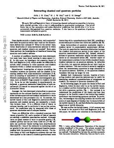
Figure 2.1: (Color online) A schematic representation of the Prize Collecting Steiner Tree problem and its local representation. Numbers next to the nodes are the distances (depths) from the root node (square node). The prize value is proportional to the darkness of the nodes. Arrows are the pointers from node to node. Distances and pointers are used to define the connectivity constraints which appear in the message-passing equations.

2.4

Derivation of the message-passing cavity equations

The algorithmic scheme we propose originates from the cavity method describe in the sec[1.2]. The starting point for the equations is the Boltzmann-Gibbs distribution: P (d, p) =

exp(−βH(p)) , Zβ

(2.5)

where (d, p) ∈ T , β is a positive parameter (a fictitious inverse temperature), and

Zβ is a normalization constant (the partition function). In the limit β → ∞ this

probability concentrates on the configurations which minimize H. Given i, j ∈ V , P the message Pji (dj , pj ) is defined as the marginal distribution (dk ,pk )k∈V \{j,i} PG(i) (d, p) on a graph G(i) , which equals to graph G minus node i and all its edges. The BP equations are derived:

Pji (dj , pj ) ∝ e−βcjpj Qkj (dj , pj ) ∝

Y

XX dk

pk

Qkj (dj , pj )

(2.6)

k∈∂j\i

Pkj (dk , pk ) gjk (dk , pk , dj , pj ) .

(2.7)


22

This assumption is correct if G is a tree, in which case (2.6)-(2.7) are exact and have a unique solution (see e.g. chapter 14.2 of [27]). The solutions of equations (2.6)-(2.7 are searched through iteration: substituting (2.7) onto (2.6) and giving a time index t+1 and t to the cavity marginals in respectively the left and right hand side of the resulting equation, this system is iterated until numerical convergence is reached. On a fixed point, the BP approximation to the marginal is computed as Pj (dj , pj ) ∝ e−βcjpj

2.4.1

Y

Qkj (dj , pj ) .

(2.8)

k∈∂j

Max-sum: β → ∞ limit

In order to take the β → ∞ limit, (2.7) can be rewritten in terms of “cavity fields” ψji (dj , pj ) = β −1 log Pji (dj , pj ) φkj (dj , pj ) = β −1 log Qkj (dj , pj ) .

(2.9) (2.10)

The BP equations take the so-called Max-sum form: ψji (dj , pj ) = −cjpj + φkj (dj , pj ) =

X

φkj (dj , pj ) + Cji

(2.11)

ψkj (dk , pk ) ,

(2.12)

k∈∂j\i

max pk ,dk :gjk (dk ,pk ,dj ,pj )=1

where Cji is an additive constant chosen to ensure maxdj ,pj ψji (dj , pj ) = 0 Computing the right side of (2.12) is in general too costly in computational terms. Fortunately, the computation can be carried out efficiently by breaking up the set over which the max is computed into smaller (possibly overlapping) subsets. We define Adkj = max ψkj (d, pk )

(2.13)

d Bkj = ψkj (d, ∗)

(2.14)

pk 6=j,∗

d Ckj = ψkj (d, j) .

(2.15)


23

Equation (2.12) can now be rewritten as: Adji =

X k∈∂j\i

d−1 d d Ekj + max −cjk − Ekj + Akj

Bji = −cj∗ + Cjid

= −cji +

(2.16)

k∈∂i\j

X

Dkj

(2.17)

d Ekj

(2.18)

k∈∂j\i

X k∈∂j\i

Dji = max max Adji , Bji d d+1 d Eji = max Cji , Dji .

(2.19) (2.20)

Using some simple efficiency tricks including computing

P

k∈∂j\i

d Ekj as

P

k∈∂j

d Ekj −

d Eki , the computation of the right side of (2.16)-(2.20) for all i ∈ ∂j can be done in a

time proportional to D|∂j|, where D is the depth bound. The overall computation time is then O(|E|D) per iteration.

2.4.2

Total fields

In order to identify the minimum cost configurations, we need to compute the total marginals, i.e. the marginals in the case in which no node has been removed from the graph. Given cavity fields, the total fields ψj (dj , pj ) = limβ→∞ β −1 log Pj (dj , pj ) can be written as: ψj (dj , pj ) = −cjpj +

X

φkj (dj , pj ) + Cj ,

(2.21)

k∈∂j

where Cj is again an additive constant that ensures maxdj ,pj ψj (dj , pj ) = 0. In def P d−1 d d terms of the above quantities we find ψj (dj , i) = Fjid = k∈∂j Ekj + −cij − Eji + Aji P def if i ∈ ∂j and ψj (dj , ∗) = Gj = −cj∗ + k∈∂j Dkj . The total fields can be interpreted as (the Max-Sum approximation to) the relative negative energy loss of

chosing a given configuration for variables pj , dj instead of their optimal choice, i.e. ψj (dj , pj ) = min {H(p0 ) : (d0 , p0 ) ∈ T }−min H(p0 ) : (d0 , p0 ) ∈ T , dj = d0j , pj = p0j .

In particular, in absence of degeneracy, the maximum of the field is attained for

values of pj , dj corresponding to the optimal energy. In our simulations, the energies computed always correspond to the tree obtained by maximizing the total fields in this way.


2.4.3

24

Iterative dynamics and reinforcement

Equations (2.16)-(2.20) can be thought as a fixed-point equation in a high dimensional euclidean space. This equation could be solved by repeated iteration of the quantities A,B, and C starting from an arbitrary initial condition, simply by adding an index (t + 1) to A, B, C in the left-hand side of (2.12) and index (t) to all other instances of A, B, C, D, E. This system converges in many cases. When it does not converge, the reinforcement is of help [52]. The resulting new Max-sum equations become:

Adji (t + 1) =

X

d Ekj (t) +

(2.22)

k∈∂j\i

d d + max −cjk − Ekj (t) + Ad−1 kj (t) + γt Fjk (t) k∈∂j\i X Bji (t + 1) = −cj∗ + Dkj (t) + γt Gj (t)

(2.23) (2.24)

k∈∂j\i

Cjid (t + 1) = −cji +

X

d Ekj (t) + γt Fjid (t)

(2.25)

k∈∂j\i

n o Dji (t) = max max Adji (t) , Bji (t) d d+1 d Eji (t) = max Cji (t) , Dji (t) X Dkj (t) + γt Gj (t) Gj (t + 1) = −cj∗ +

(2.26) (2.27) (2.28)

k∈∂j

Fjid

(t + 1) =

X k∈∂j

d Ekj

(t) + −cji − Eijd (t) + Ad−1 ij (t) +

+γt Fjid (t) .

(2.29) (2.30)

In our experiments, the equations converge for a sufficiently large γt . The strategy we adopted is, when the equations do not converge, to start with γt = 0 and slowly increase it until convergence in a linear regime γt = tρ (although other regimes are possible). The number of iterations is then found to be inversely dependent on the parameter ρ. This strategy could be interpreted as using time-averages of the MS marginals when the equations do not converge to gradually bootstrap the system into an (easier to solve) system with sufficiently large external fields. A C++ implementation of these equations can be found (in source form) on [53].


25

Note that the cost matrix (cij ) need not to be symmetric, and the same scheme could be used for directed graphs (using cji = ∞ if (i, j) ∈ E but (j, i) ∈ / E).

2.4.4

Root choice

The PCST formulation given in the introduction is unrooted. The MS equations on the other hand, need a predefined root. One way of reducing the unrooted problem to a rooted problem is to solve N = |V | different problems with all possible different rooting, and choose the one of minimum cost. This unfortunately adds a

factor N to the time complexity. Note that in the particular case in which some vertex has a large enough prize to be necessarily included in an optimal solution P (e.g. λbi > e∈E ce ), this node can simply be chosen as as root. We have devised a more efficient method for choosing the root in the general case, which we will now describe. Add an extra new node r to the graph, connected to every other node with identical edge cost µ. If µ is sufficiently large, the best energy solution is the (trivial) tree consisting in just the node r. Fortunately, a solution of the MS equations on this graph gives additional information: for each node j in the original graph, the marginal field ψj gives the relative energy shift of selecting a given parent (and then adjusting all other variables in the best possible configuration). Now for each j, consider the positive real value αj = −ψj (1, r),

that corresponds with the best attainable energy, constrained to the condition that r is the parent of j. If µ is large enough, this energy is the energy of a tree in which only j (and no other node) is connected to r (as each of these connections costs µ). But these trees are in one to one correspondence with trees rooted at j in the original graph. The smallest αj will thus identify an optimal rooting. Unfortunately the information carried by these fields is not sufficient to build the optimal tree. Therefore one needs to select the best root j and run the MS equations a second time on the original graph using this choice.

2.5

other method

We compared the performance of msgsteiner with three different algorithms: two that employ an integer linear programming strategy to find an optimal subtree,


26

namely the Lagrangian Non Delayed Relax and Cut (LNDRC) [54] and branchand-cut (DHEA) [48], and a modified version of the Goemans and Williamson algorithm (MGW)[47].

2.5.1

integer linear progamming

The goal of Integer Linear Programming (ILP) is to find an integer vector solution x∗ ∈ Zn such that: cT x∗ = min{cT x∗ | Ax ≥ b, x ∈ Zn },

(2.31)

where a matrix A ∈ Rm∗n and vector b ∈ Rm and c ∈ Rn are given. Many

graph problems can be formulated as an integer linear programming problem [55]. In general, solving (2.31) with x∗ ∈ Z is NP-Complete. The standard approach

consists in solving (2.31) for x∗ ∈ R (a relaxation of the original problem) and use the solution as a guide for some heuristics or complete algorithm for the integer case. The relaxed problem can be solved by many classical algorithms, like the Simplex Method or Interior Point methods [56]. In order to map the PCST problem in a ILP problem we introduce a variable vector z ∈ {0, 1}E and

y ∈ {0, 1}V where the component for an edge in E or for a vertex in V is one if it is included in the solution and zero otherwise. Now (2.2) can be written as H=

X e∈E

ce ze −

X

bi y i ,

(2.32)

i∈V

and the constraints Ax ≥ b in (2.31), that are used to enforce that induced sub-

graph is a tree, generally involve all or most of the variables z and y. Roughly speaking Ax ≥ b in (2.31) defines a bounded volume in the space of parameters,

i.e. a polytope. The equation to minimize is linear (2.31) so the minimum is on a vertex of this polytope. In general for hard problems, in order to ensure that each vertex of the polytope (or more in particular just the optimal vertex) is integer, a number of extra constraints that grows exponentially with the problem size may be needed [55]. DHEA and LNRDC use different techniques to tackle the problems of the enormous number of resulting constraints. Both programs are able in principle to prove the optimality of the solution (if given sufficient/exponential time), and when it


27

is not the case they are able to give a lower bound for the value of the optimum given by the the optimum of the relaxed problem.

2.5.2

Goemans-Williamson

The MGW algorithm is based on the primal-dual method for approximation algorithms [46]. The starting point is still the ILP formulation of the problem (2.31), but it employs a controlled approximation scheme that enforces the cost of any solution to be at most twice as large as the optimum one. In addition, MGW implements two different post-processing strategies, namely a pruning scheme that is able to eliminate some nodes while lowering the cost, and the computation of the minimum spanning tree in order to find an optimal rewiring of the same set of nodes. The overall running time is O(n2 log n). A complete description is available in [46].

2.6

Computational Experiments

2.6.1

Instances

Experiments were performed on several classes of instances:

• C, D and E available at [57] and derived from the Steiner problem instances of

the OR-Library [58]. This set of 120 instances was previously used as benchmark for algorithms for the PCST[58]. The solutions of these instances were obtained with the algorithms[48, 54]. The class C, D, E have respectively 500, 1000, 2000 nodes and are generated at random, with average vertex degree: 2.5, 4, 10 or 50. Every edge cost is a random integer in the interval [1, 10]. There are either 5, 10, n/6, n/4 or n/2 vertices with prizes different

from zero and random integers in the interval [1, maxprize] where maxprize is either 10 or 100. Thus, each of the classes C, D, E consists of 40 graphs. • K and P available at [57]. These instances are provided in [47]. In the first group instances are unstructured. The second group includes random

geometric instances designed to have a structure somewhat similar to street


28

maps. Also the solution of these instances were found with the algorithms [48, 54]. • H are the so-called hypercubes instances proposed in [59]. These instances

are artificially generated and they are very difficult instances for the Steiner tree problem. Graphs are d-dimensional hypercubes with d ∈ 6, ..., 12. For

each value of d, the corresponding graph has 2d vertices and d · 2d−1 edges.

We used the prized version of these instances defined in [48]. For almost all instances in this class the optimum is unknown. • i640 are the so-called incidence instances proposed in [60] for the Minimum Steiner Tree problem. These instances have 640 nodes and only the nodes in a subset K ⊆ V have prizes different from zero (in the origi-

nal problem these were terminals). The weight on each edge (i, j) is defined with a sample r from a normal distribution, rounded to an integer value with a minimum outcome of 1 and maximum outcome of 500, i.e., cij = min{max{1, round(r)}, 500}. However, to obtain a graph that is much harder to reduce by preprocessing techniques three distributions with a different mean value are used. Any edge (i, j) is incident to none, to one, or to two vertices in subset K. The mean of r is 100 for edges (i, j) with i, j ∈ / K, 200 on edges with one end vertex in K, and 300 on edges with both ends in K. Standard deviation for each of the three normal distribu-

tions is 5. In order to have prizes also on vertices we extracted uniformly from all integer in the interval between 0 and 4∗maxedge where maxedge is the maximum value of edges in the samples considered. There are 20 variants combining four different number of vertices in K (rounding to the integer √ √ value [.]): |k| = [log2 |V |], [ |V |], [2 |V |], and [|V |/4] with five edge number: |E| = [3|V |/2], 2|V |, [|V | log |V |], [2|V | log |V |], and [|V |(|V | − 1)/4]. Each variant is drawn five times, giving 100 instances.

• Class R. The last class of samples are G(n, p) random graphs with n vertices and independent edge probability p = (2ν)/(n − 1). The parameter ν is the average node degree, that was chosen as ν = 8. The weight on each edge

(i, j) can take three different value, 1, 2 and 4, with equal probability 31 . Node prizes were extracted uniformly in the interval [0, 1]. We generated different graphs with four different values of λ (λ = 1.2, 1.5, 2 or 3), see (2.2), in order to explore different regimes of solution sizes. We find that the average number of nodes that belong to the solution for λ = 1.2, 1.5, 2


29

and 3 are respectively about 14%, 33%, 51%, 67% of the total nodes in the graph. We have created twelve instances of different size for the four class of random graph, from n = 200 up to n = 4000 nodes. For each parameter set we generated ten different realizations. The total number of samples is 480.

The msgsteiner algorithm was implemented in C++ and run on a single core of an AMD Opteron Processor 6172, 2.1GHz, 8 Gb of RAM, with Linux, g++ compiler, -O3 flag activated. A C++ implementation of these equations can be found in source form on [53]. The executable of DHEA is available in [57], and in order to compare the running time we ran DHEA and msgsteiner on the same workstation. The executable of LNDRC and MGW programs was not available. We implemented the non-rooted version of MGW to compare only the optimum on the random graph instances.

2.6.2

Results

We analyzed two numeric quantities: the time to find the solution, and the gap between the cost of the solution and the best known lower bound (or the optimum solution when available) typically found with programs based on linear programming. The gap is defined as gap = 100 ·

Cost−LowerBound . lowerBound

In Table (2.1) we show the comparison between msgsteiner and the DHEA program. DHEA is able to solve exactly K, P and C, D, E instances. The worst performance of msgsteiner is on the K class, where the average gap is about 2.5%. In this class the average solution is very small as it comprises only about 4.4% of total nodes of the graph. msgsteiner seems to have most difficulty with small subgraphs. msgsteiner is able to find solutions very close to the optimum for the P class, that should be model a street network. msgsteiner is also able to find solutions very close to the optimum, with a gap inferior to 0.025% on the C, D, and E classes. In Figure (2.2) we show the gap of msgsteiner and MGW from the optimum values found by the DHEA program in the class R. msgsteiner gaps are almost negligible (always under 0.05%) and tend to zero when the size grows. MGW gaps instead are always over 1%. For intermediate size of solutions trees the gaps of MGW are over 3%.


gap (%)

4

30 0.4

(a)

3

0.3

2

0.2

1

0.1

0

0

1000

2000

3000

number of nodes

4000

0

(b) λ = 1.2 λ = 1.5 λ=2 λ=3

0

1000

|V(T)|/|V(G)| = 15% |V(T)|/|V(G)| = 33% |V(T)|/|V(G)| = 51% |V(T)|/|V(G)| = 67%

2000

3000

4000

number of nodes

Figure 2.2: (Color online) Gap from the optimum found by DHEA program of respectively (a) MGW and (b) msgsteiner as a function of the number of nodes. msgsteiner gaps are always under 0.05%. MGW gaps are always over 1% and for intermediate sizes of the solution tree the gaps of MGW are over 3%.

In Figure (2.3) we show the running time for the class R, with increasing solution tree size. In general we observe that the running time of msgsteiner grows much slower than the one of DHEA for increasing number of nodes in the graph and msgsteiner largely outperforms DHEA in computation time for large instances; furthermore the differences between the algorithms became specially and large for large expected tree solution. In at least one case DHEA could not find the optimum solution whithin the required maximum time and the msgsteiner solution was slightly better. The class i640 consists in graphs with varying number of edges and nodes, and a varying number of nodes with non-zero prize. We define K as the subset of nodes with non-zero prize. Table (2.2) shows, for each type of graph, the average time and the average gap on five different realizations of the graphs for msgsteiner and DHEA algorithms. We set the time limit to find a solution of DHEA to 2000 seconds. We observe that DHEA obtains good performance in terms of the optimality of the solution when the size of subset K is small. msgsteiner finds better result than DHEA when the size of K is sufficiently large, within a time of one or two order of magnitude smaller. Moreover DHEA seems to have difficulty to find reasonable good solution when the graph have high connectivity. We show in Table (2.3) a comparison between msgsteiner, LNDRC [54] and DHEA. The results and running time of LNDRC are taken from [54]. The computer reportedly used for the optimization is comparable with ours. We have


31

1000

5000

(a)

(b)

MSGSTEINER DHEA

1000

time (s)

100 100 10 10 1

1 200

500

1000

2000

5000

time (s)

1000

200

4000

2000

4000

1000 2000 500 number of nodes

4000

500

1000

5000

(c)

(d) 1000

100

100

10

10

1 200

1000 2000 500 number of nodes

4000

1

200

Figure 2.3: (Color online) Result on the random graphs class R. Points correspond to the running time of msgsteiner and DHEA versus graph size. The four cases show how running time behavior depends on size of the expected solution tree. The plots (a), (b), (c), (d) have respectively λ = 1.2, 1.5, 2, 3 and average value of the fraction of nodes that belongs to the solution respectively |V (T )|/|V (G)| = 0.14, 0.33, 0.51, 0.67. The quantities shown in figure are averaged over ten different realizations. Data are fitted with function y = axb . The b values found for DHEA are for (a), (b), (c), (d) respectively : 2.4, 2.8, 2.8, 2.8. BP performance is as expected roughly linear in the number of vertices. The fitted b parameters are for (a), (b), (c), (d) respectively: 1.5, 1.3, 1, 1. For instances that are large enough, the running time of msgsteiner is smaller than the one of DHEA and the difference increases with the expected solution tree.

imposed to DHEA a time limit of 6000 seconds and we show two results of msgsteiner with different values of the reinforcement parameter. The lower bound is taken from [54]. In almost all instance msgsteiner obtains better results, both in time and in quality of solution. The difference is accentuated for large instances. As expected, decreasing the reinforcement parameter allows to find lower costs at the expense of larger computation times.

Chapter 02. Optimization Group K P C D E

32

MS gap MS time (s) 2.62% 6.51 0.46% 2.31 0.006% 16.24 0.005% 35.06 0.024% 305.49

DHEA gap 0.0% 0.0% 0.0% 0.0% 0.0%

DHEA time (s) 127.97 0.18 2.30 16.12 1296.11

Size Sol 4.4% 31.4% 20.2% 20.2% 26.4%

Table 2.1: Results class KPCDE

Name time MS 0-0 0.8 0-1 2.5 0-2 100.8 0-3 1.2 0-4 37.3 1-0 1.0 1-1 2.6 1-2 90.6 1-3 1.5 1-4 33.7 2-0 0.8 2-1 4.3 2-2 149.7 2-3 1.2 2-4 39.2 3-0 1.1 3-1 3.9 3-2 112.6 3-3 1.6 3-4 33.1 mean 31.0

time DHEA 0.2 4.2 226.6 0.3 72.8 0.85 1060.1 1133.8 3.8 2000.0 0.7 2000.0 2011.1 12.0 2001.0 2.4 2001.0 2015.1 145.3 2000.5 834.6

gap MS (%) 1.3 1.0 1.4 0.05 1.8 0.3 1.2 0.7 0.8 1.8 0.1 2.2 0.8 0.2 1.9 0.3 1.7 0.8 0.2 1.2 1.0

gap DHEA (%) 0 0 0 0 0 0 1.5 0.2 0 7.8 0 11.6 14.8 0 11.2 0 5.6 4.9 0 59.9 5.9

Table 2.2: Results i640 class

2.6.3

discussion

In this chapter we compared msgsteiner, with two state-of-the art algorithms for the Prize-Collecting Steiner Problem. The Cavity Theory is expected to give asymptotically exact results on many ensembles of random graphs, so we expected it to give better performance for large instances. The comparison was performed both on randomly-generated graphs and existing benchmarks. We observed that msgsteiner finds better costs in significantly smaller times for many of the instances analyzed, and that this difference in time and quality grew with the size of the instances and their solution. We find these results encouraging in views of

Chapter 02. Optimization Name 6p 6u 7p 7u 8p 8u 9p 9u 10p 10u 11p 11u 12p 12u mean

MS(-5) gap(%) time(s) 2.2 3.5 1.5 6.4 2.3 90.2 2.2 134.1 2.4 255.5 1.8 351.1 1.8 555.6 1.9 775.8 1.7 1761.9 2.7 2468.4 1.5 972.3 2.2 5632.8 1.5 4970.8 2.0 4766.7 2.0 1624.7

33 MS(-3) gap(%) time(s) 2.6 0.6 4.3 0.7 3.9 1.7 2.2 1.8 3.4 3.8 3.3 4.9 2.3 10.8 3.3 11.1 1.7 28.0 2.7 32.2 1.6 49.3 2.6 71.9 1.6 121.4 2.4 174.1 2.7 36.6

LNDRC gap(%) time(s) 4.2 0.5 4.3 0.5 7.7 1.5 3.6 1.2 7.1 5.2 7.5 4.1 8.6 16.1 6.2 13.1 10.4 114.4 7.7 59.8 11.6 630.0 9.0 360.6 11.3 3507.7 10.0 1915.7 7.8 473.6

DHEA gap(%) time(s) 2.2 21.3 1.5 0.4 2.3 6000.3 2.2 596.4 2.3 6004.2 3.3 6000.9 22.1 6000.0 Not Found 6000.4 31.3 6000.5 Not Found 6000.6 Not Found 6003.1 Not Found 6001.5 Not Found 6009.8 Not Found 6002.3 − 4760.1

Table 2.3: Results H class

future applications to problems in biology in which optimization of networks with millions of nodes may be necessary, in particular given the conceptual simplicity of the scheme behind msgsteiner (a simple fixed-point iteration).

2.7

Post-processing and optimality

For this section we will assume unbounded depth D. Results are not easily generalizable to the bounded-D case. Results in this section apply to the non-reinforced MS equations (γt = 0). The results here are based in construction of certain trees associated with the original graph and in the fact that MS/BP equations are always exact and have a unique solution on trees [51]. Definition 1. Let {ψij } be a MS fixed-point (2.11)-(2.12), and let d, p be the de-

cisional variables associated with this fixed point, i.e. (d∗i , p∗i ) = arg max ψi (di , pi ) for the physical field ψi from (2.21). We will assume this maximum to be non degenerate. We will employ the induced subgraph S ∗ =(V ∗ , E ∗ ) defined by V ∗ = {i ∈ V : p∗i 6= ∗}∪{r} and E ∗ = {(i, p∗i ) : i ∈ V, p∗i ∈ V }. The cost of this subgraph P is H (S ∗ ) = H (p) = i∈V cip∗i . The following local optimality property of the Max-Sum-induced solution will be proven in the appendix A. It states that a MS solution is no worse than any subgraph containing a subset of the nodes.


34

Theorem 2. Given a MS fixed point {ψij } on G (unbounded D) with induced

subgraph S ∗ = (V ∗ , E ∗ ) and any subtree S 0 = (V 0 , E 0 ) ⊆ G with V 0 ⊆ V ∗ , then H (S ∗ ) ≤ H (S 0 )

This result has an easy generalization to loopy subgraphs: Corollary 3. With S ∗ as in Theorem 2, given any connected subgraph S 0 = (V 0 , E 0 ) ⊆ G with V 0 ⊆ V ∗ , then H (S ∗ ) ≤ H (S 0 ). Proof. Apply Theorem (2) to a spanning tree of S 0 . This trivially implies the following result of global optimality of the MS solution in a particular case: Corollary 4. With S ∗ = (V ∗ , E ∗ ) as in Theorem 2, if V ∗ = V then H (S ∗ ) = P CST (G)

In [47], the MGW algorithm includes two additional methods to obtain a better PCST solution: StrongPrune and Minimum Spanning Tree (MST) maintaining the same vertex set. Both methods give a substantial improvement boost to the MGW candidate computed in the first phase. A natural question may arise, does any of these two methods may help to improve the solution of MS? The answer is negative in both cases, and it is a trivial consequence of Theorem (2). Corollary 5. M ST (V ∗ , E ∩ (V ∗ × V ∗ )) = H (S ∗ ) Proof. The minimum spanning tree of (V ∗ , E ∩ (V ∗ × V ∗ )) satisfies the hypothesis of Theorem (2), so H (S ∗ ) ≤ M ST (V ∗ , E ∩ (V ∗ × V ∗ )). The converse inequality is trivially true due to the optimality of the MST.

Corollary 6. H (StrongPrune (S ∗ )) = H (S ∗ ) Proof. This is a consequence of the fact that V (StrongPrune (S ∗ )) ⊆ V (S ∗ ) = V ∗

and thus Theorem (2) applies, implying H (S ∗ ) ≤ H (StrongPrune (S ∗ )). The opposite inequality H (StrongPrune (F )) ≤ H (F ) was proved in [47].

Chapter 3 Variational Quantum Cavity Method 3.1

Introduction

In this chapter it is presented a technique that allows to compute approximate low excite states of many body quantum systems. In general it is a computationally hard task even founding the ground-state in one-dimensional quantum systems. Exact diagonalization algorithms are very helpful but they are limited to small systems due to the exponential growth of the Hilbert space with the system size [61]. For larger systems one has to resort to approximation methods, e.g., the variational quantum Monte Carlo algorithms, to study the low-energy states of the Hamiltonian [62–64]. On the other hand, one can always obtain useful insights by studying some exactly solvable mean-field models [65]. The estimation of local expectation values is of central importance in classical and quantum statistical physics in order to infer the physical state of an interacting system. This is in general a computationally hard problem especially for disordered systems displaying glassy behaviors, where approximation algorithms based on the Monte Carlo sampling could be very time consuming. At least for mean-field systems and finite-connectivity models with a locally tree-like interaction graph, the cavity method, described in the first chapter, provides efficient message-passing algorithms.

35

Chapter 03. Variational Quantum Cavity Method

36

In the work of Ramezanpour it was presented an approach that merges the technique explained in 1.4.1 for stochastic optimization problems with the variational principle of quantum mechanics, i.e. the fact that any trial wave function provides an upper bound for the ground-state energy. The problem of finding the optimal state can be recast as an optimization problem with an objective function that evaluates the energy of the system. The idea is to map the trial wave function on a Gibbs state of a classical system and to consider the set of couplings as variational parameters. Crucial in this respect is the choice of the classical systems that should be able to capture the quantum nature of the original system. Given the trial wave function, the average of the quantum Hamiltonian can be estimated by cavity method. When we work on quantum systems that have a structure different from trees, Hamiltonian averages computed by the cavity method is an estimation of the true one, so in this case the upper bound property of the Hamiltonian is lost. In the chapter 4 it is presented a different technique that solves the same optimization problems in a faster and more precise way. In order to study to the lower excited state of a system we can use the same procedure described above imposing additionally the orthogonality conditions between lower-energy eigenstates of the Hamiltonian. The main point is to write the overlap between two wave functions in the Bethe approximation, which is asymptotically exact as long as the trial wave functions can be represented by classical systems of locally tree-like interaction graphs. This allows us to replace the global orthogonality condition with some local constraints on the variational parameters and the cavity messages in the Bethe expression for the overlap. In section 3.2 the variational quantum cavity method [15] is presented. Then, in section 3.3 it s shown the method to find low energy excite states within the Bethe measure [17].

3.2

Ground state approximate wave function

Given a Hamiltonian H and a trial wave function |ψ(P )i, we have hψ(P )|H|ψ(P )i ≥ Eg where Eg is the ground-state energy of H and P denotes a set of parameters

characterizing the trial wave function. To find the optimal parameters we define


37

the following optimization problem: Z=

X

e−βopt hψ(P )|H|ψ(P )i ,

(3.1)

P

where eventually one is interested in the limit βopt → ∞. Note that βopt is just the

inverse of a fictitious temperature and has nothing to do with the physical temperature. In the equation (3.2) we have to perform a sum over a set of parameters that change the average value of a energy function defined, at least for systems addressed in this thesis, over discrete variables. This problems is very close to a stochastic optimization problems showed in sec 1.4.1, as well as the technics I will show in the next sections to solve it. Assume H = H0 + H1 , where H0 is diagonal in the orthonormal basis |σi; H0

and H1 are Hermitian operators with real eigenvalues and orthonormal eigenvectors. The trial wave function is represented in this representation as |ψ(P )i = P 2 σ ψ(σ; P )|σi. The coefficients ψ(σ; P ) are complex numbers, and |ψ(σ; P )| =

ρ(σ; P ) is a normalized probability distribution over σ. The average energy can be written as hψ(P )|H|ψ(P )i =

X

=

X

σ

|ψ(σ; P )|2 [E0 (σ) + E1 (σ)]

(3.2)

ρ(σ; P ) [E0 (σ) + E1 (σ)] ,

(3.3)

σ

where E0 (σ) ≡ hσ|H0 |σi,

E1 (σ) ≡ Re

( X ψ ∗ (σ 0 ; P ) σ0

ψ ∗ (σ; P )

) hσ 0 |H1 |σi .

(3.4)

We consider ρ(σ; P ) ≡ |ψ(σ; P )|2 as a probability measure in a classical sys-

tem and compute the above average quantities within the Bethe approximation. Q For ψ(σ; P ) ∝ a∈Ec φa (σ ∂a ; Pa ), the classical measure is given by ρ(σ; P ) ∝ Q ∂a 2 ∂a a |φa (σ ; Pa )| with the set of classical interactions Ec ≡ {φa (σ )|a = 1, . . . , A}. Here ∂a is the subset of variables that appear in φa . We write the BP equation


38

(1.44) over this classical systems: µi→a (σi ) ∝ µa→i (σi ) ∝

Y

µb→i (σi ),

(3.5)

b∈∂i\a

X σ ∂a\i

|φa (σ ∂a ; Pa )|2

Y

µj→a (σj ).

(3.6)

j∈∂a\i

The average of any local quantity like E0 and E1 can be written as a function of the BP cavity marginals (or messages). Therefore, the optimization problem reads Z=

XX P

e−βopt hE0 iρ −βopt hE1 iµ 1BP ,

(3.7)

µ

where the indicator function 1BP ensures that the messages µ satisfy the BP equations, like shown for stochastic optimization problem in sec.1.4.1. In the case of multiple BP fixed points the above partition function would be concentrated on one minimum of the average energy for βopt → ∞. More accurate average energies are obtained, of course, by considering replica symmetry breaking, for instance the

1RSB equations considered in sec.1.4, and working with a probability distribution of the BP fixed points.

3.2.1

Quantum ising model

We consider the quantum Ising model with Hamiltonian H = H0 + H1 where P P x H0 = − (ij)∈Eq Jij σiz σjz and H1 = − N i=1 hi σi . The Jij are real parameter describing the interactions in the z direction between spins, and the hi are also real parameter representing transverse external fields on the x direction. The interaction graph is defined by Eq , and N is the size of the system. The σ x,y,z are the

standard Pauli matrices. The states |σi are the 2N configurations of the σ z spins. P P In this case hσ|H0 |σi = − (ij)∈Eq Jij σi σj and hσ 0 |H1 |σi = − i hi δσi ,−σi0 δσ\i,σ0 \i , where δa,b is the the delta of Dirac between two variable (a, b). We consider

only real parameter in the Hamiltonian, then the ground state wave function can be always describe by a real function. Moreover, if h > 0, the ground state is a positive wave function1 . In this thesis we consider only positive h values of transverse external field. 1

giustify


3.2.2

39

Pairwise model

For the trial wave functions we take a pairwise model plus external field ansatz: P

e

ψ(σ; P ) = P

P

σe

P

i

Bi σi +

i

2Bi σi +

(ij)∈Ec

P

Kij σi σj

(ij)∈Ec

2Kij σi σj

1/2 ,

(3.8)

with real parameters P = {Bi , Kij |i = 1, . . . , N, (ij) ∈ Ec }. This results in the Gibbs measure µ(σ; P ) = |a(σ; P )|2 of a classical spin-glass model with external

fields 2Bi and couplings 2Kij . Notice that the classical interaction graph Ec could be different from the quantum one Eq . For simplicity, in the following we will

assume that the two coincide as happens in zero transverse fields; better representations could be obtained by adding the higher order neighbors to Ec . Given the classical measure, the BP equations read: ! µi→j (σi ) ∝ e2Bi σi

Y

X

k∈∂i\j

σk

e2Kik σi σk µk→i (σk )

≡ BP i→j ,

(3.9)

where ∂i refers to the set of spins interacting with spin i in Ec . Figure 3.1 displays

the set of variables and interactions in the classical interaction graph. Having the

cavity marginals, the average of local energies eij ≡ −Jij σiz σjz and ei ≡ −hi σix read heij iµ = −Jij hei iµ = −hi

X

σi σj µij (σi , σj ),

(3.10)

σi ,σj

X

P

e−2Bi σi −

j∈∂i

2Kij σi σj

µi,∂i (σi , σ∂i ),

(3.11)

σi ,σ∂i

with the local BP marginals µij (σi , σj ) ∝ e2Kij σi σj µi→j (σi )µj→i (σj ) and µi,∂i (σi , σ∂i ) ∝ Q e2Bi σi j∈∂i [e2Kij σi σj µj→i (σj )]. The above average energies define the Boltzmann weight e−βopt hE0 iµ −βopt hE1 iµ for a given configuration of the variational parameters and the BP messages; see figure 3.1. The cavity marginals of the parameters (including the BP messages) can be written in a higher-level Bethe approximation, resembling the one-step RSB equations (sec.[1.4]): Mi→j (Kij , µij ) ∝ e−βopt heij iµ

X Bi {Kik ,µik | k∈∂i\j}

e−βopt hei iµ

Y k∈∂i\j

Mk→i (Kik , µik )1BP (i) , (3.12)


40

Bi

σi µ i−−>j Kij

σj

Bi , BP Kij

µ ij

Mi−−>j Bj

Figure 3.1: (top) The interaction graphs of the classical system representing the trial wave function and (bottom) the resulting variational problem. The variables are shown with solid circles, and the interactions are shown with open polygons.

Q where for brevity we defined µij ≡ {µi→j , µj→i } and 1BP (i) ≡ j∈∂i δ(µi→j − P P BP i→j ). The Bethe free energy is given by F = i Fi − (ij)∈Ec Fij with e−βopt Fi ≡ e−βopt Fij ≡

X

e−βopt hei iµ

Bi ,{Kij ,µij |j∈∂i}

X

Y

Mj→i (Kij , µij )1BP (i) ,

(3.13)

j∈∂i

e+βopt heij iµ Mi→j (Kij , µij )Mj→i (Kij , µij ),

(3.14)

Kij ,µij

Notice that in the last equation we have the positive sign in the exponential to count correctly the energy contribution heij iµ . The βopt → ∞ limit of the above equations, taking the scaling Mi→j (Kij , µij ) = eβopt Mi→j (Kij ,µij ) , read

Mi→j (Kij , µij ) = −heij iµ +

max

Bi ,{Kik ,µik |k∈∂i\j}:1BP (i)

  

−hei iµ +

X k∈∂i\j

Mk→i (Kik , µik )

  

(3.15)

,


41

they are the Max-Sum/BP equations like in the stochastic optimization (sec.[1.4.1]). P P The minimum energy is given by Eg = limβopt →∞ F = −( i ei − (ij)∈Ec eij ) with

the local energy shifts

( ei ≡

max

Bi ,{Kij ,µij |j∈∂i}:1BP (i)

)

−hei iµ +

X j∈∂i

Mj→i (Kij , µij ) ,

eij ≡ max {heij iµ + Mi→j (Kij , µij ) + Mj→i (Kij , µij )} . Kij ,µij

(3.16) (3.17)

Before solving the above equations we will consider some simpler cases.

3.2.3

Zero couplings: Mean field solution

In the zeroth order of the approximation we take Kij = 0 for any edge (ij). Q This is a mean-field approximation with a factorized measure µ(σ) = i µi (σi ), where µi (σi ) = e2Bi σi /[2 cosh(2Bi )]. Then using equations (3.10) and (3.11) we obtain the average local energies: heij iµ = −Jij tanh(2Bi ) tanh(2Bj ) and hei iµ =

−hi / cosh(2Bi ); therefore hψ(B)|H|ψ(B)i = −

X (ij)∈Eq

Jij tanh(2Bi ) tanh(2Bj ) −

X i

hi . cosh(2Bi )

(3.18)

Here we write directly the MaxSum equations that can be used to estimate the optimal parameters and the minimum average energy: Mi→j (Bi ) = −hei iµ +

X k∈∂i\j

max {−heik iµ + Mk→i (Bk )} . Bk

(3.19)

Then we find the optimal paramters by maximizing the local MaxSum weights: ( Bi∗

3.2.4

= arg max −hei iµ + Bi

) X j∈∂i

max {−heij iµ + Mj→i (Bj )} . Bj

(3.20)

Zero fields: Symmetric solution

As long as the fields Bi are zero we have always a symmetric solution µi→j (σi ) = 1/2 to the BP equations in the classical system. This gives the average local


42

energies: heij iµ = −Jij tanh(2Kij ) and hei iµ = −hi /[ hψ(K)|H|ψ(K)i = −

X (ij)∈Eq

Jij tanh(2Kij ) −

Q

j∈∂i

X Q i

cosh(2Kij )], and

hi . j∈∂i cosh(2Kij )

(3.21)

The resulting MaxSum equations are

Mi→j (Kij ) = −heij iµ +

max

 

{Kik |k∈∂i\j} 

−hei iµ +

X k∈∂i\j

Mk→i (Kik )

 

,

(3.22)



and the optimal couplings are estimated by Kij∗ = arg max {heij iµ + Mi→j (Kij ) + Mj→i (Kij )} . Kij

(3.23)

Notice that here we have hσiz i = 0, which is not the case in the ordered phase.

In addition, the symmetric solution does not give an accurate average energy when replica symmetry is broken, which may happen for large couplings in the

classical system; the Bethe approximation works well when distant spins are nearly independent, whereas the symmetric solution does not respect this property in an RSB phase. To get around this problem one can work with the nontrivial BP fixed points, e.g., by demanding a total magnetization of magnitude greater than δm 1. At the same time one may need to limit the range of couplings to |Kij | < Kmax in order to avoid dominance by very large couplings.

3.2.5

General solution

In general to solve the MaxSum-BP equations we have to work with discrete fields Bl ∈ {lδB|l = −LB , . . . , LB }, couplings Kl ∈ {lδK|l = −LK , . . . , LK }, and BP

cavity fields νl ∈ {lδν|l = −Lν , . . . , Lν }. The BP cavity fields νi→j are defined by µi→j (σi ) ∝ eνi→j σi . An exhaustive solution of the MaxSum-BP equations would

take a time of order N d(2LB )[(2LK )(2Lν )]d where d is the maximum degree in Ec .

Notice that given the couplings Kij and the input BP messages νj→i around spin i, one obtains νi→j for any value of Bi from the BP equations. The above equations can be solved more efficiently (for large degrees) by using a convolution function of four variables (needed to compute hei iµ in the MaxSum-BP equations) resulting

in a time complexity of order N d(2LK )(2Lν )6 ; see appendix in the article[]. In the following instead we use a computationally easier but approximate way of


43

solving the equations by restricting the domain of variables: We start by assigning a small number of randomly selected states Sij = {(Kij1 , νij1 ), . . . , (KijS , νijS )} to each

variable (Kij , νij ). Then we run the MaxSum-BP equations with these restricted

search spaces to converge the equations and sort the states in Sij according to their MaxSum-BP weights: wij (Kijl , νijl ) = heij iµ + Mi→j (Kijl , νijl ) + Mj→i (Kijl , νijl ).

(3.24)

Next we update the search spaces by replacing the states having smaller weights with some other ones generated randomly but close to the best state observed during the algorithm. The above two steps are repeated to find better search spaces and therefore parameters. The algorithm performance would depend on the size of the search spaces, approaching the correct one for S → ∞. The search spaces at the beginning are chosen randomly therefore we introduce a tolerance δν to accept those BP messages that satisfy the BP equations within ±δν. One may start from a large tolerance and decrease it slowly after each update of the search spaces. The mean-field solution mentioned before can provide a good initial point for the search spaces.

3.2.6

Numerical results

3.2.6.1

Random coupling chain

First, we consider a spin chain in uniform and positive transverse field but with random couplings. In figure 3.2 we compare the results obtained by the above approximations with the exact ones obtained by the modified Lanczos method [66]. As expected, the mean-field ansatz is better than the symmetric solution in the ordered phase where the local magnetizations are nonzero. The reverse happens in the disordered phase and even in the ordered phase close to the transition point where the local magnetizations are still small. The two limiting behaviors are therefore displayed in the general solution.


44

Chain, N=20, J=Gaussian: Lanczos MF, LB=1000, δB=0.005 SS, LK=1000, δK=0.005 GS, S=100, δν=0.01 N=1000, GS, S=100, δν=0.01

-0.5 -1

1 -2

0.8 0.6

qz

Eg/N

-1.5

-2.5

0.4 0.2

-3

0 0

1

2

3

-3.5 0

0.5

1

1.5

2

2.5

3

h 1

0.8

mx

0.6

0.4 Chain, N=20, J=Gaussian: Lanczos MF, LB=1000, δB=0.005 SS, LK=1000, δK=0.005 GS, S=100, δν=0.01 N=1000, GS, S=100, δν=0.01

0.2

0 0

0.5

1

1.5 h

2

2.5

3

Figure 3.2: Comparing the exact results with those of the mean-field (MF), the symmetric solution (SS) and the general solution (GS) in a single instance of the quantum Ising model in transverse field h on a chain of size N = 20. For comparison we also display the GS results for N = 1000. Here Eg and mx are the ground-state energy and magnetization in the x direction,P respectively. The inset shows the Edwards-Anderson order parameter qz = ( i hσiz i2 )/N . The couplings Jij are Gaussian random numbers of mean zero and variance one. δB, δK, and δν are the sizes of bins in the discrete representation of the parameters, and S is the number of states in the restricted domains. The data for GS are obtained by restricting the search algorithm to total magnetizations of magnitude greater than δm = 0.05.

Chapter 03. Variational Quantum Cavity Method 3.2.6.2

45

Random graph

As another example we study the same model on a single instance of random regular graphs where each spin interacts with a fixed number of other randomly selected spins. The results displayed in figure 3.3 show similar behaviors observed above, except that in the ordered phase the symmetric solution gives a lower ground state energy than the exact one. As explained before, this is due to the poor estimation of the average energy by the symmetric solution when there are multiple BP fixed points. Moreover, due to the loops and small size of the system we find larger deviations from the exact data compared to the chain model. Similar qualitative behaviors are observed in ferromagnetic (Jij = 1) and ±J spinglass (Jij = ±1 with equal probability) models on a random regular graph of degree

d = 3. In the ferromagnetic case, a reasonable trial wave function is obtained by taking Bi = B and Kij = K. This simplification allows us to find easily the optimal parameters, and so the critical field hfc erro ∼ 2.29 in the thermodynamic

limit. Figure 3.4 displays the phase diagram of the ferromagnetic model obtained in this way. For the ±J spin-glass model, the general solution on single instances

' 2.0. The corresponding values in the thermodynamic of size N = 1000 gives h±J c

limit given in Refs. [13] and [12] are: hfc erro ∼ 2.23 and h±J ∼ 1.77. c

3.3

Low temperature excitations

In this section we use the variational quantum cavity method, shown in the previous section, to find approximate solutions for the exited-states of the transverse Ising model. The main point of this study is to write the overlap between two wave functions in the Bethe approximation, which is asymptotically exact as long as the trial wave functions can be represented by classical systems of locally treelike interaction graphs. This allows us to replace the global orthogonality condition with some local constraints on the variational parameters and the cavity messages in the Bethe expression for the overlap. In summary, given an appropriate trial wave function, we evaluate the Hamiltonian expectation in the subspace of wave functions orthogonal to the lower-energy states of the Hamiltonian and find an estimation of the optimal variational parameters, all within the Bethe approximation. We implemented it by a local message-passing algorithm.


-0.5

RRG d=3, N=20, J=Gaussian: Lanczos MF, LB=1000, δB=0.005 SS, LK=1000, δK=0.005 GS, S=50, δν=0.01 N=1000, GS, S=30, δν=0.02

-1 -1.5

Eg/N

46

-2 1 0.8

-2.5

qz

0.6

-3

0.4 0.2

-3.5

0 0

1

2

3

-4 0

0.5

1

1.5

2

2.5

3

3.5

h 1

0.8

mx

0.6

0.4 RRG d=3, N=20, J=Gaussian: Lanczos MF, LB=1000, δB=0.005 SS, LK=1000, δK=0.005 GS, S=50, δν=0.01 N=1000, GS, S=30, δν=0.02

0.2

0 0

0.5

1

1.5

2 h

2.5

3

3.5

4

Figure 3.3: The quantum Ising model in transverse field h on a random regular graph (RRG) of degree d = 3 and size N = 20. For comparison we also display the GS results for N = 1000. The couplings Jij are Gaussian random numbers of mean zero and variance one. The data for GS are obtained by restricting the search algorithm to total magnetizations of magnitude greater than δm = 0.05 and couplings of magnitude less than Kmax = 1.


-1.5

47

RRG d=3: Mean Field ansatz Ising ansatz Quantum Cavity (T=0.1)

-2

Eg/N

-2.5 1 -3

0.8 mx

0.6

-3.5

0.4 0.2

-4

0 0

1

2

3

4

5

-4.5 0

0.5

1

1.5

2

2.5

3

3.5

4

h 1

RRG d=3: Mean Field ansatz Ising ansatz Quantum Cavity (T=0.1)

0.8

mz

0.6

0.4

0.2

0 0

0.5

1

1.5

2 h

2.5

3

3.5

4

Figure 3.4: The quantum Ising model with ferromagnetic interactions (Jij = 1) in transverse field h on RRG of degree d = 3. The results of homogeneous mean field Bi = B and Ising (Bi = B, Kij = K) trial wave functions are compared with the results of the quantum cavity method [13] for a small temperature in the thermodynamic limit.


48

Note that, usually, for large and disordered systems we do not have the exact ground-state of the system. The best that we can do is to find a good variational wave function that represent the low-energy state of the system. Obviously, an excited state that is orthogonal to an approximate ground state does not necessarily provide an upper bound for the excited-state energy. There are, of course, other ways to find the excited states that do not rely on the orthogonality to a priori known ground state, but we found the above procedure more amenable to the cavity method that we are going to use in this paper. Nevertheless, any orthogonal set of quantum states defines a subspace of wave vectors that according to the Courant min-max theorem [67] can be used to find some upper bounds for the Hamiltonian eigenvalues.

3.3.1

Orthogonality constraints

Let us denote by |Ψn (P n )i the nth trial wave function that minimizes the average energy hΨn (P n )|H|Ψn (P n )i conditioned on the orthogonality constraints

hΨn (P n )|Ψm (P m )i = 0 for m = 0, . . . , n − 1. The corresponding classical systems

are represented by measures µn (σ; P n ). In the following we are going to satisfy the orthogonality constraints within the Bethe approximation, hΨn (P n )|Ψm (P m )i =

X σ

ψn∗ (σ; P n )ψm (σ; P m ) ' e−(

P

i

Fi +

P

a

P Fa − (ia) Fia )

= 0, (3.25)

where Fi , Fa , and Fia are the free energy changes by adding variable node i, interaction node a, and link (ia) to the complex measure νn,m (σ; P n , P m ) ∝ Q ψn∗ (σ; P n )ψm (σ; P m ) ∝ a φ∗a (σ ∂a ; Pan )φa (σ ∂a ; Pam ). These quantities are given by (see sec.1.3.2),

e−Fi =

XY

νa→i (σi ),

(3.26)

σi a∈∂i

e−Fa =

X

φ∗a (σ ∂a ; Pan )φa (σ ∂a ; Pam )

σ ∂a

e−Fia =

X

Y

νi→a (σi )

(3.27)

i∈∂a

νi→a (σi )νa→i (σi ),

(3.28)

σi

where the cavity marginals νi→a (σi ) and νa→i (σi ) satisfy the BP equations for the complex measure νn,m (σ; P n , P m ). Thus, to have orthogonality it is enough to


49

have e−Fa = 0 for some a. This defines a constraint on the parameter Pan given P m. In summary, to estimate the average energy and to satisfy the orthogonality constraints we need to know the BP marginals of the classical measure µn and {νn,m |m = 0, . . . , n − 1}. In addition, we have to choose the set of constrained pa-

rameters An ≡ {am |m = 0 . . . , n − 1} for the orthogonality constraints e−Fam = 0. In this paper we will use a greedy strategy to construct An , by choosing the parameters that at least locally minimize the energy expectation. Finally, the problem of minimizing over the variational parameters is: Zn =

X

X

Pn

µn ,{νn,m }

IBP

Y

In,m e−βopt hE(σ)iµn ,

(3.29)

m=0,...,n−1

where for βopt → ∞ the Gibbs measure is concentrated on the optimal parameters.

The indicator functions 1BP and 1n,m ensure that the messages µn , {νn,m } satisfy

the BP equations and the states n and m are orthogonal. Starting from n = 0, one can find the other states one by one after solving the above optimization problem. One may find an approximate solution to the above problem by a two-stage algorithm: Given {P m |m = 0, . . . , n − 1} and an arbitrary set of the constrained

parameters An , we run BP to find the set of marginals {νn,m |m = 0, . . . , n − 1}.

These are used to fix the constrained parameters in An to satisfy the orthogonality constraints. Then we minimize the average energy hE(σ)iµn over the remaining parameters. The above two stages are repeated to converge the algorithm.

3.3.2

The mean-field approximation

Let us start with the mean-field (MF) approximation, where the trial wave functions are represented by the product states: ψ(σ; B) ∝

Y

eBi σi ,

(3.30)

i R

with complex parameters Bi . This results to ei (σi ) = −hi e−2Bi σi cos(2BiI σi ) and Q R the following classical measure µ(σ; B) ∝ i e2Bi σi . By superscripts R and I we mean the real and imaginary part of the parameters. Given the above measure we


50

find hei (σi )iµ = −hi

cos(2BiI ) , cosh(2BiR )

(3.31)

heij (σi , σj )iµ = −Jij tanh(2BiR ) tanh(2BjR ).

(3.32)

We see that for non-negative hi the average energy is minimized by setting BiI = 0. Therefore, as long as we are interested in the ground state, we can set the imaginary parts to zero. In this case, the variational problem reads Z0 =

X

e−βopt

P

(ij)∈Eq heij iµ −βopt

P

i hei iµ

,

(3.33)

B

The cavity marginals of the parameters in the Bethe approximation are ! Mi→j (Bi ) ∝ e−βopt hei iµ

Y

X

k∈∂i\j

Bk

e−βopt heik iµ Mk→i (Bk ) .

(3.34)

For βopt → ∞ and scaling Mi→j (Bi ) = e−βopt Mi→j (Bi ) we find the Min-Sum equations [68]:

Mi→j (Bi ) = hei iµ +

X k∈∂i\j

min {heik iµ + Mk→i (Bk )} . Bk

(3.35)

The equations are solved by iteration starting from random initial messages. After each iteration we subtract a constant from the messages to have minBi Mi→j (Bi ) = 0. Then we find the optimal parameters by minimizing the local Min-Sum weights, ( Bi0 = arg min hei iµ + Bi

) X j∈∂i

min {heij iµ + Mj→i (Bj )} . Bj

(3.36)

Note that in the MF approximation the orthogonality condition reads hΨn (B n )|Ψm (B m )i ∝

Y

cosh(Bin∗ + Bim ) = 0,

(3.37)

i

thus, it is enough to have cosh(Bin∗ +Bim ) = 0 for some i. This means BinR = −BimR

and BinI − BimI = π/2. Therefore, the nth excited state can be obtained by the


51

following set of constraints: ( In,m =

BinR + BimR = 0, m m

(3.38)

= π2 , − BimI BinI m m

for m = 0, . . . , n − 1. The index im is chosen to minimize the local energy heim (σi )iµn . Then, one can use the same Min-Sum equations as above to minimize

over the remaining parameters. In this way we can find at most N orthogonal product states of minimum energies En . Given the states |Ψm (B m )i for m = 0, . . . , n, we can easily compute the Hamil0

tonian matrix elements Hmm0 ≡ hΨm (B m )|H|Ψm0 (B m )i, which for arbitrary parameters read Hmm0 =

Y

0

cosh(Bim∗ + Bim ) 0 (cosh(2BimR ) cosh(2Bim R ))1/2

i    X m0  m∗ X cosh(Bi − Bi ) 0 0 × − Jij tanh(Bim∗ + Bim ) tanh(Bjm∗ + Bjm ) − hi . 0  cosh(Bim∗ + Bim )  i

(ij)∈Eq

(3.39) One can diagonalize the Hamiltonian in the subspace spanned by the above states to obtain the eigenvalues λm . Then, using the min-max principle, we know that λn is an upper bound for the nth eigenvalue of the Hamiltonian. Indeed, we found that in this case λn ' En for large N as the off-diagonal matrix elements Hmm0 decay exponentially with the size of system.

Notice that instead of imposing the orthogonality exactly we could ask for an exponentially small overlap hΨn (B n )|Ψm (B m )i < N by demanding cosh(Bin∗ + Bim ) < ≤ 1, (cosh(2BinR ) cosh(2BimR ))1/2

(3.40)

for all i, which can easily be imposed in the above Min-Sum equations. Indeed to apply the min-max theorem we do not need a set of orthogonal states [67]; according to the theorem, the nth eigenvalue is given by minSn+1 max|ψi∈Sn+1 :hψ|ψi=1 hψ|H|ψi

where Sn+1 is any subspace of dimension n + 1.


3.3.3

52

Beyond the mean-field approximation

We can do better than the MF approximation by adding the local two-body or Jastrow interactions [69] to the trial wave functions: ψ(σ; P ) ∝

Y

Y

φi (σi )

i

φij (σi , σj ),

(3.41)

(ij)∈Ec

with φi (σi ) ≡ eBi σi ,

φij (σi , σj ) ≡ eKij σi σj .

(3.42)

For simplicity we are going to assume Ec = Eq . As a result, we obtain Rσ − i

ei (σi , σ ∂i ) = −hi e−2Bi

P

j∈∂i

Rσ σ 2Kij i j

cos(2BiI σi +

X

2KijI σi σj ).

(3.43)

j∈∂i

The average energy is computed with respect to the following classical measure Q Q µ(σ) ∝ i |φi (σi )|2 (ij)∈Ec |φij (σi , σj )|2 . To estimate the average energies heij (σi , σj )iµ

and hei (σi , σ ∂i )iµ we need the following local marginals

1 |φij (σi , σj )|2 µi→j (σi )µj→i (σj ), Zij Y 1 µi,∂i (σi , σ ∂i ) = |φi (σi )|2 |φij (σi , σj )|2 µj→i (σj ), Zi,∂i j∈∂i µij (σi , σj ) =

(3.44) (3.45)

given in terms of the cavity marginals ! µi→j (σi ) ∝ |φi (σi )|2

Y

X

k∈∂i\j

σk

|φik (σi , σk )|2 µk→i (σk ) .

(3.46)

For Bi = 0 we can simplify the equations by taking the symmetric (or paramagnetic) solution of the BP equations. This is of course exact for a tree classical interaction graph Ec . Then, the average local energies are given by hei (σi , σ ∂i )iµ = −hi

Y j∈∂i

cos(2KijI ) cosh(2KijR )

heij (σi , σj )iµ = −Jij tanh(2KijR ).

! ,

(3.47) (3.48)


53

The resulting Min-Sum equations are  

  X Mi→j (Kij ) = min hei iµ + (heik iµ + Mk→i (Kik )) ,  {Kik |k∈∂i\j} 

(3.49)

k∈∂i\j

and the optimal couplings are estimated by Kij0 = arg min {heij iµ + Mi→j (Kij ) + Mj→i (Kij )} .

(3.50)

Kij

The orthogonality condition for two symmetric states reads hΨn (K n )|Ψm (K m )i ∝

X

P

e

n∗ m (ij)∈Ec (Kij +Kij )σi σj

σ

∝

Y

cosh(Kijn∗ + Kijm ) = 0,

(ij)∈Ec

(3.51) using the symmetric solution of the BP equations. Thus, to have orthogonality we need cosh(Kijn∗ + Kijm ) = 0 for some link (ij). That is, for the nth excited state we have the following set of constraints: ( In,m =

= 0, + KimR KinR m jm m jm

(3.52)

KinI − KimI = π2 , m jm m jm

for m = 0, . . . , n − 1. The link (im jm ) is chosen to minimize the local energy

heim jm iµn . Then, one can use the same Min-Sum equations as above to minimize

over the remaining parameters. The number of orthogonal states that we can find in this way is limited by the number of the coupling parameters in the classical system which for a tree structure is N − 1. The Hamiltonian matrix elements are

given by

0

Hmm0 =

Y (ij)∈Eq

×

  

−

X (ij)∈Eq

cosh(Kijm∗ + Kijm ) 0 (cosh(2KijmR ) cosh(2Kijm R ))1/2 0

Jij tanh(Kijm∗ + Kijm ) −

X i

hi

Y j∈∂i

!

cosh(Kijm∗ cosh(Kijm∗

− +

0 Kijm ) 0 Kijm )

! 

. (3.53)



Similarly, we can make more general orthogonal states |Ψn (B n , K n )i and |Ψn (B m , K m )i P

by choosing Bin such that for the complex measure νnm ∝ e

n∗ m i (Bi +Bi )σi +

P

n∗ m (ij)∈Ec (Kij +Kij )σi σj

Chapter 03. Variational Quantum Cavity Method -15

-10

RT, N=20: exact MF S

-20

54 RT, N=20: exact MFoMF SoS ToT

-20 -30

-25 16

E1

E0

-40 -30

-50

-23 -35 -24

-60

-25

-70

E1-E0

12 8 4

-40

0.8

0.9

0

1

0

-45

1

2

3

4

-80 0

0.5

1 h

1.5

2

0

0.5

1

1.5

2 h

2.5

3

3.5

4

Figure 3.5: The ground-state and excited-state energies (E0 and E1 ) for the transverse Ising model on a random tree (RT) of size N = 20 with random Gaussian couplings Jij of mean zero and variance one in a uniform transverse field hi = h. The exact results are compared with the upper bounds that are obtained by a minimal energy subspace spanned by product states (MFoMF), symmetric states (SoS), and tree states (ToT).

we have e∆Fi = 0 for some i. This gives P 2(Bin∗ +Bim )

e

=−

Y

σj

P j∈∂i

σj

n∗ +K m )σ j ij

e−(Kij

n∗ +K m )σ j ij

e(Kij

νj→i (σj )

νj→i (σj )

! .

(3.54)

The node i can be chosen in a greedy way to minimize hei (σi , σ ∂i )iµn in the meanfield approximation. Here it is more difficult to minimize the average energy

hE(σ)iµn , which depends not only on the variational parameters but also on the BP cavity marginals µi→j (σi ). More precisely, the Min-Sum equations read

Mi→j (Kij , µij ) =

 

min (i)

Bi ,{Kik ,µik |k∈∂i\j}:IBP



hei iµ +

X k∈∂i\j

  (heik iµ + Mk→i (Kik , µik )) ,  (3.55)

where µij ≡ (µi→j , µj→i ). Note that the minimum in the right hand side is conditioned on satisfying the local BP equations. The reader can find more details in Ref. [15].

3.3.4

Results

Let us start with a small system to compare the above approximations with the exact results for the ground and excited states. We take a random tree with random Gaussian couplings Jij of mean zero and variance one in uniform transverse

Chapter 03. Variational Quantum Cavity Method -0.8

55

10

1D, Jij=1: MF S

1D, Jij=1, N=100: MFoMF ToT (h-hc)1.04 +/- 0.005

-1 8

6

-1.4

E1-E0

E0/N

-1.2

-1.6

4

-1.8 2 -2 -2.2

0 0

0.2

0.4

0.6

0.8

1 h

1.2

1.4

1.6

1.8

2

0

1

2

3

4

5

h

Figure 3.6: Left panel: The ground-state energy density (E0 /N ) for the onedimensional (1D) transverse Ising model with uniform and ferromagnetic couplings (Jij = 1) obtained by the product states (MF) and the symmetric states (S) in the thermodynamic limit. Right panel: The energy gap E1 − E0 obtained by the product states (MFoMF) and tree states (TOT) for the same model with N = 100 spins. In both the cases the gap is non-analytic at the corresponding phase transition point, but it is non-vanishing close to the transition due to the local nature of the orthogonality constraints. -0.8

-0.8

RT, N=1000: MF S T

-1 -1.2

-1.2

-1.4

-1.05

-1.6

-1.1

-1.6

-1.8

-1.15

-1.8

-2

-1.2

E1/N

E0/N

RT, N=1000: MFoMF SoS ToT

-1

-1.4

E1-E0

8

4

0

-2 0.7

0.8

0.9

0

-2.2

1

2

3

-2.2 0

0.5

1 h

1.5

2

0

0.5

1 h

1.5

2

Figure 3.7: The ground-state and excited-state energy densities (E0 /N and E1 /N ) for the transverse Ising model on a random tree (RT) of size N = 1000 with random Gaussian couplings Jij of mean zero and variance one in a uniform transverse field hi = h. We compare the upper bounds that are obtained by a minimal energy subspace spanned by product states (MFoMF), symmetric states (SoS), and tree states (ToT).

fields hi = h. This system displays a phase transition from the ordered phase for P h < hc with a nonzero Edwards-Anderson order parameter q ≡ i hσiz i2 /N to a disordered phase for h > hc .

As Fig. 3.5 shows, we obtain better ground-state energies with the product and symmetric states in the ordered and disordered phases, respectively. While the product states allow for a nonzero magnetization, the symmetric states have by definition zero magnetization and therefore more appropriate to represent the disordered ground state. Indeed, an estimate of the transition point can be obtained

Chapter 03. Variational Quantum Cavity Method -1

-1

2D, N=20: exact MF

2D, N=20: exact MFoMF

-1.5

E1/N

-1.5

E0/N

56

-2

6

-2

E1-E0 4

-2.5

2

-2.5

0 0 -3

1

2

3

-3 0

0.5

1

1.5 h

2

2.5

3

0

0.5

1

1.5 h

2

2.5

3

Figure 3.8: The ground-state and excited-state energy densities (E0 /N and E1 /N ) for the transverse Ising model on a two-dimensional (2D) square lattice of size N = 4×5 with random Gaussian couplings Jij of mean zero and variance one in a uniform transverse field hi = h. The exact results are compared with the upper bounds that are obtained by a minimal energy subspace spanned by product states (MFoMF).

by comparing the ground-state energies that are computed by the product and symmetric states. Figure 3.6 displays these energies for the one-dimensional transverse Ising model with ferromagnetic couplings. Nevertheless, for small system sizes we always obtain better energies for the excited state by a minimal energy subspace of the product states. In Fig. 3.5 we also display the results obtained by more general trial wave functions having a tree structure defined by Ec = Eq . As

expected, we obtain much better upper bounds by introducing both the variational parameters Bi and Kij . Figure 3.7 shows the results for a larger number of spins. Here, in the disordered phase we find better upper bounds for the excited-state energy by the symmetric trial wave function. This is due to the presence of very small couplings that reduce the cost of the orthogonality constraint. Finally, we present the MF results for the transverse Ising model in a two-dimensional square lattice. In Fig. 3.8 we compare the upper bounds for the ground and excited states with the exact ones in a small lattice.

3.4

Discussion

In the section 3.3 it is shown a generalized variational quantum cavity method to study low-temperature excitations of quantum systems within the Bethe approximation. We constructed orthogonal sets of minimal energy quantum states, where the Hamiltonian matrix elements can be computed exactly to obtain some upper


57

bounds for the Hamiltonian eigenvalues. For more general trial wave functions we have only an approximate estimation of the Hamiltonian matrix elements but the estimation is expected to be asymptotically exact as long as the trial wave functions are represented by locally tree-like classical interaction graphs. And finally, the method can also be extended to include some appropriate global interactions in the trial wave functions that are essential to deal with the fermion sign problem [70].

Chapter 4 Variational Quantum Density Matrix 4.1

Introduction

This last chapter is divided in two parts. In the first one a new method to find approximate wave functions is described. The wave function is approximated in the same way presented in chapter 3, i.e. by a product of local terms. The algorithm proposed applies iteratively the imaginary time evolution operator to find the ground state wave function. This algorithm is able to find better solution and in more efficient way than the variational quantum cavity method presented in the previous chapter. The imaginary time approach slowly modifies the parameters during the evolution in order to minimize the energy. This procedure permit to avoid the binning of the parameters used in the variational cavity method. This allows to use better approximate wave functions. The whole procedure is presented in the density matrix formalism because it is easier to extend it to finite temperature systems. In the second part of the chapter we discuss a method to find approximate density matrices at finite temperature. In this case the density matrix is approximate by a product of local reduced density matrices. The algorithm performs an annealing in temperature, starting from infinite temperature. We force the density matrix, at each small temperature reduction, to remain a product of local reduced density matrices. The results obtained are encouraging, but the accumulation of the error 58

Chapter 04. Variational Quantum Density Matrix

59

during the annealing process, due to the ansaltz of the density matrix, reduces the precision of the algorithm. Improved results can be obtained, from both algorithms presented in this chapter, using better expansions of the density matrix and working with generalize belief propagation equations [71]. This should be the case, above all, when we deal with square lattice problems [72]. In section 4.2 it is shown the imaginary time evolution of a Bethe density matrix. In sec. 4.3 it is described the finite temperature algorithms .

4.2

Imaginary time evolution

In this chapter I work directly with the density matrix formalism instead of the wave matrix formalism developed in chapter 3. Let’s consider an N body hamiltonian H with real parameters. Taking a base |σi, the density operator at zero temperature (isolated system) ρ is defined as: ρ = |ψi hψ| =

X σ,σ 0

C ∗ (σ)C(σ 0 ) |σi hσ 0 |

(4.1)

where we have expanded the wave function |ψi over a complete base {|σi} and

C(σ) = hψ |σi. If the wave function |ψi is normalized, the diagonal elements of the density matrix are probabilities, they define a measure. We proceed now in the same way of the variational quantum cavity method, see section 3.2. We have two different graphs, one Eq generated by the physical interactions due to the hamiltonian, and another graph Ec generated by the approximated measure. From now, I will consider Ec = Eq = E. Let me approximate the probability distribution

|C(σ)|2 with a Bethe form:

|C(σ)|2 ∼

Y i

ψi2 (σi )

Y ij

ψij2 (σi , σj ) . ψi2 (σi ) ψj2 (σj )

(4.2)

We consider ψi and ψij positive real functions, for simplicity. The ψi2 (σi ) = ρi (σi ) and ψij2 (σi , σj ) = ρij (σi , σj ) are respectively the one body and two body marginals


60

of the system. We define a zero temperature Bethe density matrix as: ρ (σ, σ 0 ) =

Y

1 2

1 2

ρi (σi ) ρi (σi0 )

i

Y ij

1 1 ρij2 (σi , σj ) ρij2 σi0 , σj0 1 1 1 1 ρi2 (σi ) ρi2 σj0 ρi2 (σj ) ρj2 σj0

(4.3)

When the interaction graph of Ec generated by a zero temperature Bethe density matrix is a tree, it is easy to show that the following identities hold1 : ρi (σi ) =

X σ\σi

ρij (σi , σj ) =

hσ| ρ |σi =

X σ\σi σj

X

ρ (σ, σ)

σ\σi

X

hσ| ρ |σi =

(4.4) ρ (σ, σ) .

σ\σi σj

More accurate zero temperature density matrices can be obtained by considering interactions between a larger number of variables, for example, 1

ρ(σ; σ 0 ) =

Y

1

1

ρij (σi , σj ) 2 ρij (σi0 , σj0 ) 2

Y i

(ij)∈Ec

1

0 2 ) ρi∂i (σi , σ∂i ) 2 ρi∂i (σi0 , σ∂i Q 1 1 , 2 ρ (σ 0 , σ 0 ) 2 ρ (σ , σ ) ik i k ik i k k∈∂i

(4.5)

where σ∂i = {σj |j ∈ ∂i}, and ∂i denotes the neighborhood set of i in the interaction graph Ec . The same identity equations (4.4) hold for the measure (4.5) in the case

of tree interaction graph Ec . We have also the following one: ρi∂i (σi , σ∂i ) =

X σ\σi ,σ∂i

4.2.1

hσ| ρ |σi =

X

ρ (σ, σ) .

(4.6)

σ\σi ,σ∂i

Imaginary time evolutions of a Bethe density matrix.

The imaginary time evolution is a technique that, in principle, allows to compute the ground state of quantum systems. The idea is to apply to a trail density matrix the imaginary time evolution operator e−tH . The excited states are exponentially suppressed in the limit of t → ∞. Let’s consider a density matrix ρ and let’s apply the imaginary time operator to it: e−tH ρe−tH =

X n,m

∗ e−tH Cm Cn |En i hEm | e−tH =

X n,m

∗ e−t(En +Em ) Cm Cn |En i hEm |

(4.7) 1

This identity can be derived considering the normalizations and marginalization constraints over the marginals ρi (σi ) and ρij (σi , σj ), and starting the trace over the variables from leafs.


61

where we have expanded over a base where the hamiltonian is diagonal. Taking the limit of t → ∞ we obtain: lim e−tH ρe−tH ≈ e−2tEg |Cg |2 |Eg i hEg |

t→∞

(4.8)

where the |Eg i is the ground state of the system. If we apply, iteratively, the

operator e−H to a trial density matrix and if the initial trial density matrix has an overlap different from zero with the ground state, the final outcome, at least approximatively, is the ground state. We want to apply iteratively the imaginary time evolution operator e−H in order to find an approximated ground state matrix. Let’s consider, for simplicity, a zero temperature Bethe density matrix at imaginary time t: q ρtij (σi , σj ) ρtij σi0 , σj0 Yp Y q ρt (σ, σ 0 ) = ρti (σi ) ρti (σi0 ) ρti (σi ) ρti σj0 ρti (σj ) ρtj σj0 i ij

(4.9)

the density matrix at time t + reads: ρt+ =

e−H ρt e−H T r{e−H ρt e−H }

(4.10)

where I normalized the expression (4.7). Now we assume that also the density matrix ρt+ has a Bethe form and so we compute the quantities ρt+ and ρt+ i ij through the formula(4.4). We need to compute the marginal probabilities ρi (σi ) and ρij (σi ; σj ) of the following system: T r{ρ+t } =

X

∝

X

=

X

=

X

σ

σ

σ

σ,σ 0

hσ| ρt+ |σi

(4.11)

hσ| e−H ρt e−H |σi

(4.12)

hσ| e−2H ρt |σi

(4.13)

hσ| e−2H |σ 0 i hσ 0 | ρt |σi

(4.14)

where in the third line I used the ciclic property of trace, and in the fourth I inserted P the identity operator 1 = σ0 |σ 0 i hσ 0 |. The marginals can be computed in the

limit of 1. In effect, let’s consider a quantum interaction graph Eq generated

by an hamiltonian H, the hσ| e−H |σ 0 i can be decomposed, by a Suzuky-Trotter


62

expansion [73, 74], in a product of functions that have the same graph structure of Eq . Then if the hamiltonian H has local interactions, also hσ| e−H |σ 0 i is composed

by products of local functions [75]. The eq.(4.11) is a product of local quantities and the marginal of this system can be computed by the BP equations. In the next section this procedure is applied to the transverse Ising model.

4.2.2

Tranverse ising model

P Consider the transverse field Ising model with Hamiltonian H = (ij)∈Eq Hij + P z z x i Hi where Hij ≡ −Jij σi σj , Hi ≡ −hi σi , and i = 1, . . . , N labels the sites in the quantum interaction graph Eq . The σix,y,z are the standard Pauli matrices. We

assume that hi > 0. In the following we will work in the σ z representation with orthonormal basis |σi ≡ |σ1 σ2 · · · σN i. The Suzuky-Trotter [73, 74] expansion allows to simplify the exponential of two non commutative quantities. In the case of the exponential of the transverse Ising hamiltonian we can write: e−H =

Y

z z

eJij σi σj /2

Y

x

ehi σi

i

(ij)∈Eq

z z

Y

eJij σi σj /2 + O(3 ).

(4.15)

(ij)∈Eq

The matrix element hσ| e−H |σ 0 i with the approximation above is: hσ| e−H |σ 0 i ≈

Y

wi (σi , σi0 )

i

Y

wij (σi , σj ; σi0 , σj0 )

(4.16)

(ij)∈Eq

where 0 0

wij (σi , σj ; σi0 , σj0 ) ≡ eJij (σi σj +σi σj )/2 ,

wi (σi , σi0 ) ≡ cosh(hi )δσi ,σi0 + sinh(hi )δσi ,−σi0 .

(4.17) (4.18)

Taking a Bethe zero temperature density matrix (4.9) at imaginary time t we have to find marginals at time t + of the following probability distribution: ρ+t (σ) =

X σ0

hσ| e−2H |σ 0 i hσ 0 | ρt |σi =

q ρtij (σi , σj ) ρtij σi0 , σj0 Y XY p wij (σi , σj ; σi0 , σj0 ) q = wi (σi , σi0 ) ρti (σi ) ρti (σi0 ) . ρti (σi ) ρti σj0 ρti (σj ) ρtj σj0 i σ0 (ij)∈Eq (4.19)


63

{σ1 . . . σN }

µi→j

� {σ1� . . . σN } Figure 4.1: In this figure it’s shown a 1 dimension two layers system. The messages µi→j group the two layers variables.

It is a two layers classic system, see fig. 4.1. Then, the BP equations over the system are: q 0 ρtij ρtij Y X n+1 0 wi wij q µi→j (σj σj ) = µnk→i (σi σi0 ) 0 ρtj ρtj k∈∂i\j σi σi

(4.20)

0 where the index n refers to the iteration of BP equations, and ρtij ≡ ρtij σi0 , σj0 .

Given the set of fixed point messages {µ∗i→j } of the eq.(4.20), the marginals can

be computed by the following formulas: ρt+ i (σi ) =

X

wi

q Y 0 ρtj ρtj µ∗j→i (σi σi0 )

σi0 t+ ρij (σi , σj ) =

X

(4.21)

j∈∂i

q Y Y 0 wij ρtij ρtij µ∗p→i (σi σi0 ) µ∗q→j (σj σj0 ).

σi0 ,σj0

p∈∂i\j

(4.22)

q∈∂j\i

We can summarize the procedure of finding the zero temperature Bethe density matrix by the following steps: 1. Initialize the marginals ρ0i and ρ0ij with a flat or random distribution. 2. Run the BP equations (4.20) until convergence. 3. Update the marginals, eq.(4.21). 4. Return to point 2 until the marginals converge.


64

In general we are looking for the fixed point solution of the set of marginals {ρi , ρij

and messages µi→j of the equations (4.21) and (4.20). The procedure above can be simplified when we consider homogenous systems where we assume that each one-body, two-body marginals and the messages are the same in the whole system. We can consider the fixed point equations for both marginals and BP equations at the same time. The problem of finding the zero temperature Bethe density matrix reduces to find the quantities ρi ρij and µ that solves the following set of equations:  q 0  ρij ρij  X    µ(σj σj0 ) = wi wij q µd−1 (σi σi0 )   0  ρj ρj  σi σi0    X q 0 ρi (σi ) = wi ρj ρj µd (σi σi0 )    σi0   q  X  0   ρ (σ , σ ) = w ρij ρij µd−1 (σi σi0 )µd−1 (σj σj0 )  ij i j ij   0 0

(4.23)

σi ,σj

where d is the number of neighbors of one node. In the next subsection I will show numerical results obtained by c++ programs that implement the procedure described above for different approximated measures: mean-field, Bethe measure eq.(4.3) and near neighbors region eq.(4.5). The programs can take as input whatever transverse Ising model hamiltonian. The only restriction is due to the convergence problems of BP equations over particular interaction graphs. Moreover when we deal with interaction graphs with loops, the average quantities computed are Bethe approximations of the real ones.

4.2.3

Numerical results

The first question that we face is: is this procedure able to really minimize the approximate wave function? In figure 4.2 are shown the energies of a transverse Ising chain computed by a zero temperature pairwise density matrix eq.(4.3). These energies are compared with those found by the variational quantum cavity method with the same structure of the wave function. As we can see from the plot 4.2, there is no difference between the two energies. The graphs 4.4 and 4.3 are the magnetizations respectively on chain and on random regular graph of degree three computed by imaginary time evolution. The blue curve is the magnetization computed by mean-field approximation, the red one is the pairwise density matrix eq.(4.3), and the green one is computed by neighbors


65

region eq.(4.5). The exact transition point is located at hc = 1 and hc = 2.232 [13] respectively for chain and for random regular graph with degree three. The critical transition fields found by the neighbors region zero temperature density matrix are closer to the correct ones than those found by pairwise and mean-field approximations (see captions of the figures 4.4 and 4.3 for precise values of the critical fields). Moreover we run the algorithm on small disorder system in order to compare the energies on loopy graphs to the exact one found by brute force diagonalization of the hamiltonian. We consider the gaps between the exact energies Eex and those found by imaginary time evolution with pairwise Epw and neighbor region Enr density matrix approximations. The gap is defined as 100 ∗ (Eex − Eapprox )/Eex .

In the fig 4.5 we show the gaps computed between the exact energies and those found by imaginary time evolution of two different matrix approximations on a 2d lattice with 20 spins (4 times 5 spins) with periodic boundary conditions. In this case the Jij = 1 and the transverse fields hi are random numbers uniformly

distributed in [0, h]. In the same plot the magnetizations M z is shown (dashed lines). We can note that the gaps are always under 0.5. They differer from zero only near the quantum critical point where the magnetization in the z direction drops to zero. Also in this case using larger regions improve the results.

4.3

Annealing of quantum systems

In this section we face the problem to find approximate density matrices at finite temperature T. The equilibrium density matrix at inverse finite temperature β should satisfy the following equation [76]: ∂ρ(β) = −Hρ ∂β

with

ρ(0) = 1

(4.24)

where H is the hamiltonian of the system. Then giving the density matrix at inverse temperature β, ρβ , we may write: ρβ+ =

e−H ρβ Z β+

(4.25)


66

Energy density of chain 0 Quantum cavity method Imaginary time evolution

Energy density

-0,5

-1

-1,5

-2

-2,5

-3

0

0,25

0,5

0,75

1

1,25

1,5

1,75

2

hx Figure 4.2: In this figure it is shown the energy density found on chain with Jij = 1 with two different methods that minimize a trial density matrix in the form eq.(4.3). The blue line is computed by the quantum cavity method presented in the chapter 3 and the red one by imaginary time evolution. There is no significant difference between them. The imaginary time step used is = 10−3

where Z β+ = T r{e−H ρβ } is a normalization constant. We want to give an ap-

proximate description of the density matrix that is locally and globally consistent on tree structures. The idea is to write the density matrix as a product of reduced density matrices. In the mean-field approximation the density matrix is simply Q approximated by ρ(σ; σ 0 ) = i ρi (σi ; σi0 ). In the Bethe approximation we may write the density matrix as ρ(σ; σ 0 ) =

Y i

ρi (σi ; σi0 )

Y (ij)∈E

ρij (σi , σj ; σi0 , σj0 ) , ρi (σi ; σi0 )ρj (σj ; σj0 )

(4.26)

for a locally tree-like interaction graph Ec that could be different from the quantum

interaction graph Eq . Here we consider Ec = Eq = E. Note that this is an ansatz for the matrix elements of ρ that is Hermitian but not necessarily semi-positive. In appendix B we see that when the interaction graph E is a tree and the reduced


67

Chain 1 0,9 0,8

z

M =

0,7 0,6 0,5

0,4 0,3

0,2 0,1 0

0

0,1

0,2

0,3

0,4

0,5

0,6

0,7

0,8

0,9

1

1,1

1,2

1,3

1,4

1,5

hx Figure 4.3: The plot shows the magnetization M = hσ z i of a chain with Jij = 1 and varying hx . The number of spins are N = 50 with periodic boundary conditions. The imaginary time step used is = 10−3 . The red line is the Bethe zero temperature density matrix (pw) eq.(4.3). The green one is the neighbors region zero temperature density matrix (nn) eq.(4.5). The critical fields found nn are respectively hpw c = 1.22 and hc = 1.12. The exact one is hc = 1.

density matrices ρij and ρi are locally consistent we have ρij = Tr\i,j ρ and ρi = Tr\i ρ. More accurate density matrices can be obtained by considering interactions between a larger number of variables, for example, ρ(σ; σ 0 ) =

Y (ij)∈E

ρij (σi , σj ; σi0 , σj0 )

Y i

ρ (σ , σ ; σ 0 , σ 0 ) Q i∂i i ∂i i 0∂i 0 , k∈∂i ρik (σi , σk ; σi , σk )

(4.27)

where σ∂i = {σj |j ∈ ∂i}, and ∂i denotes the neighborhood set of i in the interaction

graph E. In the same lines of appendix B we can show that for tree interaction

graphs E and locally consistent ρi∂i and ρij we have ρi∂i = Tr\i,∂i ρ and ρij = Tr\i,j ρ.


68

Random regular graph degree 3

Figure 4.4: The plot shows the magnetization M = hσ z i of a random regular graph with degree three with Jij = 1 and varying hx . The number of spins are N = 50. The imaginary time step used is = 10−3 . The blue line is the mean-field zero temperature density matrix, the red one is the Bethe zero temperature density matrix eq.(4.3) and the green one is the neighbors region zero temperature density eq.(4.5). The critical fields found are respectively nn hmf = 3, hpw c c = 2.29 and hc = 2.25. The exact one is hc = 2.232.

4.3.1

Annealing algorithm of quantum Ising model

In order to find the density matrix describing the equilibrium state of the system at temperature T = 1/β we start from the density matrix at infinite temperature ρ ∝ I and we decrease slowly the temperature in an annealing process. We use a

similar procedure described for the imaginary time evolution in subsection 4.2.2. The density matrix ρβ+ reads: ρβ+ (σ; σ 0 ) ∝

XY σ 00

i

wi (σi , σi00 )

Y (ij)∈Eq

wij (σi , σj ; σi00 , σj00 )ρβ (σ 00 ; σ 0 ),

(4.28)


69

2D random fields lattice 1

0,8

0,3

0,6

0,2

0,4

0,1

0,2

z

0,4

M =

Gaps [%]

neighbors region pairwise

0

0

1

2

3

4

5

6

7

8

9

10

11

0 12

h Figure 4.5: The plot shows the gaps (100 ∗ (Eex − Eapprox )/Eex ) between the exact energies and two different approximate energies found by imaginary time evolution. The red one is founded using a Bethe density matrix eq. (4.3), and the green one by neighbors region density matrix eq. (4.5). Dashed lines show the magnetizations M z =< σ z > of the same approximate density matrices. We note that the gaps are different from zero only near the quantum transition point, where the magnetizations drop to zero. The gaps are always below 0.5. Better results are obtained with neighbors region approximate density matrix.

where 00 00

wij (σi , σj ; σi00 , σj00 ) ≡ eJij (σi σj +σi σj )/2 ,

wi (σi , σi00 ) ≡ cosh(hi )δσi ,σi00 + sinh(hi )δσi ,−σi00 .

Let us start from the mean-field approximation of the density matrix ρ =

(4.29) (4.30)

Q

i

ρi

where in each step the density matrix is updated as follows ρβ+ (σ; σ 0 ) ∝

i Y XYh wi (σi , σi00 )ρβi (σi00 ; σi0 ) wij (σi , σj ; σi00 , σj00 ). σ 00

i

(ij)∈Eq

(4.31)


70

Then, within the Bethe approximation the reduced density matrices ρβ+ = Tr\i ρβ+ i are obtained by   h iY X X  ρβ+ (σi ; σi0 ) ∝ wi (σi , σi00 )ρβi (σi00 ; σi0 ) wij (σi , σj ; σi00 , σj00 )µj→i (σj , σj00 ) . i σi00

j∈∂i

σj00

(4.32) Here ∂i denotes the neighborhood set of i in Eq , and the cavity marginals µi→j (σi , σi00 ) are determined by the BP equations for the Gibbs measure ρβ+ (σ; σ),

  i Y X Xh  wik (σi , σk ; σi00 , σk00 )µk→i (σk , σk00 ) . wi (σi , σi00 )ρβi (σi00 ; σi ) µi→j (σi , σi00 ) ∝ σi00

k∈∂i\j

σk00

(4.33) Given the ρi and the weights wi , wij , we solve the above equations by iteration starting from random initial cavity marginals µi→j (σi , σi00 ), and use the cavity marginals to find the lower-temperature reduced density matrices ρβ+ . The equai tions showed in this section is very close to those presented in sec. 4.2 for the imaginary time evolution algorithm. Indeed the imaginary time procedure, started from a flat distribution, can be seen as an annealing process where at each step we force the density matrix to have a zero temperature structure like in the equation (4.3).The main difference between the two procedures relies in the form of the density matrix: the diagonal elements are parametrized in a different way.

4.3.2

Numerical result

The figure 4.6 shows the phase transition points that are obtained in this way for the ferromagnetic transverse Ising model on a random regular graph. Unfortunately, the errors in each step of the annealing algorithm accumulate, giving rise to larger and larger errors as we decrease the temperature. The point is that at each step of the annealing process we assume that the present density matrix ρ is the right density matrix at inverse temperature β which is correct only if we work with the most general density matrix representation. As a result the density matrix that we obtain is not the optimal one; indeed, minimizing the free energy directly at inverse temperature β with the same density matrix representation could result to smaller free energies [14]. However, as the figure shows, the error is reduced by enlarging the space of the trial density matrices. In appendix C we give the update equations for neighbor region density matrices.


71

2,00 1,80

pairwise neighbor region exact

1,60 1,40 1,20

Tc 1,00 0,80 0,60 0,40 0,20 0,00

0,25

0,50

0,75

1,00

1,25

1,50

x

1,75

2,00

2,25

2,50

2,75

3,00

h

Figure 4.6: Comparing the phase transition points in the transverse Ising model (Jij = 1 and hi = h) on a random regular graph of degree K = 3 obtained by the annealing algorithm (for system size N = 50 and different density matrix representations) and the exact solution of the path integral quantum cavity method [13] in the thermodynamic limit.

Appendix A Post-processing and optimality proofs Before tackling the proof of the Theorem 2, we will need the following definitions and a technical result. Definition 7. (Computation tree) The computation tree is a cover of the graph G, in the following sense: it is an (infinite) tree TG along with an application

π : TG → G that satisfies (a) π is surjective and (b) π|i∪∂i : i ∪ ∂i → π (i ∪ ∂i) is a graph isomorphism for every i ∈ TG . It can be explicitly constructed as the graph

of non-backtracking paths in G starting on a given node v0 , with two paths being connected iff the longest one is identical to the other except for an additional final node (and edge). Up to graph isomorphisms, this tree does not depend on the choice v0 . The (finite) tree TG (t, v0 ) is defined by the radius t ball centered around vo in

TG . Alternatively, it can be directly constructed as the graph of non-backtracking

paths of length up to t starting on v0 , with two paths being connected iff the

longest one is identical to the other except for an additional final node (and edge). Clearly the finite computation tree depends strongly on the choice of v0 For both computation trees, edge weights (and node prizes) will be lifted (transported) naturally as cij = cπ(i)π(j) . Lifting edge constraints by gij = gπ(i)π(j) defines a (R, D)-PCSF problem with R = π −1 ({r}) on TG . On TG (t, v0 ) instead, it gives a slightly relaxed (R, D)-PCSF 72

Appendix A. optimality proofs

73

problem in which leaf nodes can point to neighbors in G that are not present in TG . For convenience, let us extend π by setting π (∗) = ∗. Remark 8. As TG (t, v) is a tree, the Max-Sum equations are exact and have a unique fixed point in TG (t, v)[27].

Lemma 9. Any Max-Sum fixed point in a graph G can be naturally lifted to a Max-Sum fixed point in TG . Moreover, any Max-Sum fixed point can be naturally lifted to a Max-Sum fixed point over a slightly modified TG (t, v) with extra cost terms only on leaves.

Proof. As Max-Sum equations are local and the two graphs are locally isomorphic, given a fixed point {ψij }(i,j)∈E , the messages Ψij = ψπ(i)π(j) satisfy the fixed point equations on TG . On TG (t, v) the Max-Sum equations are satisfied everywhere ex-

cept possibly on leaf nodes (where the graphs are not locally isomorphic). Given a leaf i attached with edge (i, j), add an energy term −Ei (di pi ) = ψπ(i)π(j) (di , π (pi )).

Now Max-Sum equations are satisfied everywhere on for this modified cost function.

Now we proceed to prove Theorem 2

A.0.3

Proof of Theorem 2

Proof. Assume S 0 oriented towards the root node r, i.e. defining a parenthood 0

vector (p0i )i∈V 0 , such that E 0 = {(i, pi ) : i ∈ V 0 \ {r}}. Consider the subgraph

S = (VS , ES ) of TG (N + 1, r) induced by S ∗ , i.e. defined by VS = {v : π (v) ∈ V ∗ },

ES = {(i, j) : (π (i) , π (j)) ∈ E ∗ }.

It can be easily proven that the connected component in S of the root node of TG (N + 1, r) is a tree S 00 isomorphic to S ∗ (see [51]). Denote by {p∗ } the decisional variables induced by S ∗ and by {p0 } the ones induced by S 0 . The parenthood assignment

qi =

 p 0

i ∈ VS 00

p ∗

i∈ / VS 00

i i

satisfies qi 6= ∗ if qj = i (as V 0 ⊆ V ∗ ) and so depths di can be assigned so as

to verify all gij constraints in TG (N + 1, r). Now the cost associated with q is P P P P P ∗ ∗ ∗ ∗ H (q) = i∈VS00 cip0i + i∈V / S 00 cipi ≥ i∈TG (N +1,r) cipi = i∈VS 00 cipi + i∈V / S 00 cipi

Appendix A. optimality proofs

74

due to the optimality of the MS solution p∗ in the computation tree (this is because MS is always exact on a tree). This implies clearly that H (S ∗ ) ≤ H (S 0 ).

Appendix B Locally and globally consistent reduced density matrices Consider the following Bethe ansatz for the density matrix ρ(σ; σ 0 ) =

Y

ρi (σi ; σi0 )

i

Y (ij)∈E

ρij (σi , σj ; σi0 , σj0 ) . ρi (σi ; σi0 )ρj (σj ; σj0 )

(B.1)

Here we prove that when E is a tree and the reduced density matrices are locally consistent we have ρij = Tr\i,j ρ and ρi = Tr\i ρ.

Let us start from computing Trρ to show that ρ is trace normalized when ρi = Trj ρij and Trρi = Trρij = 1. Expanding the trace we have Z = Trρ =

XY σ

ρi (σi ; σi )

i

Y (ij)∈E

ρij (σi , σj ; σi , σj ) . ρi (σi ; σi )ρj (σj ; σj )

(B.2)

For tree structures we can compute the above sum recursively 

Z=

X σi

 X ρij (σi , σj ; σi , σj )  ρi (σi ; σi ) Zj→i (σj ) , ρ (σ ; σ )ρ (σ ; σ ) i i i j j j σ j∈∂i Y

(B.3)

j

using the Bethe equations [27], Zi→j (σi ) = ρi (σi ; σi )

Y k∈∂i\j

! X ρik (σi , σk ; σi , σk ) Zk→i (σk ) , ρ (σ ; σ )ρ (σ ; σ ) i i i k k k σ k

75

(B.4)

Appendix B. Locally and globally density matrices

76

where Zi→j (σi ) is the cavity partition function when spin i has state σi . Note that for the leaves we have Zi→j (σi ) = ρi (σi ; σi ) and from the marginalization relations ρi = Trj ρij we find Zi→j (σi ) = ρi (σi ; σi ) for all the cavity partition functions. P Therefore we obtain Z = σi ρi (σi ; σi ) = 1. To compute the one-body reduced density matrices we use again the recursive equations to write 

 X ρij (σi , σj ; σ 0 , σj ) i  Zj→i (σj ) . hσi |Tr\i ρ|σi0 i = ρi (σi ; σi0 ) 0 ρ (σ ; σ )ρ (σ ; σ ) i i j j j i σ j∈∂i Y

(B.5)

j

But Zj→i (σj ) = ρj (σj ; σj ) which along with the marginalization relations give Tr\i ρ = ρi . Similarly, one can prove that Tr\i,j ρ = ρij thanks to the tree interaction graph E and the consistency of the local density matrices ρi and ρij . One can easily extend the above arguments to more general density matrices with higher order interactions ρ(σ; σ 0 ) =

Y i

ρi (σi ; σi0 )

Y ρa (σ∂a ; σ 0 ) ∂a Q , 0 ρ (σ i∈∂a i i ; σi ) a

(B.6)

as long as the bipartite graph representing the dependency of the interactions to the variables is a tree. Here σ∂a ≡ {σi |i ∈ ∂a} and ∂a defines the set of variables

in interaction a.

Appendix C Computing the reduced density matrices in the annealing algorithm Consider the following Bethe ansatz for the density matrix 0

ρ(σ; σ ) =

Y i

ρi (σi ; σi0 )

Y (ij)∈E

ρij (σi , σj ; σi0 , σj0 ) . ρi (σi ; σi0 )ρj (σj ; σj0 )

(C.1)

In each step of the annealing process we need to compute the local reduced density matrices given the updated density matrix ρ˜(σ; σ 0 ) ∝

i Y h XYh ρij (σi00 , σj00 ; σi0 , σj0 ) i wi (σi , σi00 )ρi (σi00 ; σi0 ) wij (σi , σj ; σi00 , σj00 ) . 00 0 00 0 ρ (σ ; σ )ρ (σ ; σ ) i i i i j j 00 i σ (ij)∈E

(C.2) The local density matrix ρ˜ij = Tr\i,j ρ˜ is obtained from the above expression after summing over the σk = σk0 for k 6= i, j. For tree interaction graphs E this sum

can be computed by considering the cavity messages that the boundary variables

77

Appendix C. annealing algorithm

78

∂(ij) receive from the other parts of the system in addition to the local weights, ρ˜ij (σi , σj ; σi0 , σj0 ) ∝ × wi (σi , σi00 ) × wj (σj , σj00 )

X

wij (σi , σj ; σi00 , σj00 )ρij (σi00 , σj00 ; σi0 , σj0 )

σi00 ,σj00

Y hX k∈∂i\j

σk ,σk00

Y hX k∈∂j\i

σk ,σk00

wik (σi , σk ; σi00 , σk00 )

i ρik (σi00 , σk00 ; σi0 , σk ) 00 ) µ (σ ; σ k→i k k ρi (σi00 ; σi0 )ρk (σk00 ; σk )

wjk (σj , σk ; σj00 , σk00 )

i ρjk (σj00 , σk00 ; σj0 , σk ) 00 µ (σ ; σ ) k→j k k . ρj (σj00 ; σj0 )ρk (σk00 ; σk ) (C.3)

Here the cavity messages µi→j are determined recursively by the Bethe equations, µi→j (σi ; σi00 ) ∝ wi (σi ; σi00 )ρi (σi00 ; σi ) i Y hX ρik (σi00 , σk00 ; σi , σk ) 00 × wik (σi , σk ; σi00 , σk00 ) µ (σ ; σ ) k→i k k . (C.4) ρi (σi00 ; σi )ρk (σk00 ; σk ) 00 k∈∂i\j

σk ,σk

Bibliography [1] P. W. Anderson. More is different. Science, 177(4047):393–396, August 1972. ISSN 0036-8075, 1095-9203. doi: 10.1126/science.177.4047.393. URL http: //www.sciencemag.org/content/177/4047/393. PMID: 17796623. [2] Marc Mézard, Giorgio Parisi, and Miguel Virasoro. Spin Glass Theory and Beyond.

World Scientific Publishing Company, September 1987.

ISBN

9971501163. [3] M. Mézard, G. Parisi, and R. Zecchina. Analytic and algorithmic solution of random satisfiability problems. Science, 297(5582):812–815, August 2002. ISSN 0036-8075, 1095-9203. doi: 10.1126/science.1073287. URL http:// www.sciencemag.org/content/297/5582/812. PMID: 12089451. [4] A. Braunstein, M. Mézard, and R. Zecchina. algorithm for satisfiability. 201–226, 2005.

Survey propagation: An

Random Structures & Algorithms, 27(2):

ISSN 1098-2418.

doi: 10.1002/rsa.20057.

URL http:

//onlinelibrary.wiley.com/doi/10.1002/rsa.20057/abstract. [5] A. Braunstein, R. Mulet, A. Pagnani, M. Weigt, and R. Zecchina. Polynomial iterative algorithms for coloring and analyzing random graphs. Physical Review E, 68(3):036702, September 2003. doi: 10.1103/PhysRevE.68.036702. URL http://link.aps.org/doi/10.1103/PhysRevE.68.036702. [6] Christos H Papadimitriou. Reading, Mass., 1994.

Computational complexity.

Addison-Wesley,

ISBN 0201530821 9780201530827 0020153082

9780020153085. [7] Christos H Papadimitriou and Kenneth Steiglitz. Combinatorial optimization: algorithms and complexity. Prentice Hall, Englewood Cliffs, N.J., 1982. ISBN 0131524623 9780131524620 0486402584 9780486402581.

79

Bibliography

80

[8] Indaco Biazzo, Alfredo Braunstein, and Riccardo Zecchina. Performance of a cavity-method-based algorithm for the prize-collecting steiner tree problem on graphs.

Physical Review E, 86(2):026706, August 2012.

doi:

10.1103/PhysRevE.86.026706. URL http://link.aps.org/doi/10.1103/ PhysRevE.86.026706. [9] GB Dantzig. Maximization of a linear function of variables subject to linear inequalities, in activity analysis of production and allocation. Wiley, 1951. [10] L. De Cesare, K. Lukierska Walasek, and K. Walasek. Cavity-field approach to quantum spin glasses: The ising spin glass in a transverse field. Physical Review B, 45(14):8127–8130, April 1992. doi: 10.1103/PhysRevB.45.8127. URL http://link.aps.org/doi/10.1103/PhysRevB.45.8127. [11] M.S. Leifer and D. Poulin. Quantum graphical models and belief propagation. Annals of Physics, 323(8):1899–1946, August 2008. ISSN 00034916. doi: 10.1016/j.aop.2007.10.001. URL http://www.sciencedirect. com/science/article/pii/S0003491607001509. [12] C. Laumann, A. Scardicchio, and S. L. Sondhi. Cavity method for quantum spin glasses on the bethe lattice. Physical Review B, 78(13):134424, October 2008. doi: 10.1103/PhysRevB.78.134424. URL http://link.aps.org/doi/ 10.1103/PhysRevB.78.134424. [13] Florent Krzakala, Alberto Rosso, Guilhem Semerjian, and Francesco Zamponi. Path-integral representation for quantum spin models: Application to the quantum cavity method and monte carlo simulations. Physical Review B (Condensed Matter and Materials Physics), 78(13):134428, 2008. doi: 10.1103/PhysRevB.78.134428. URL http://link.aps.org/abstract/PRB/ v78/e134428. [14] L. B. Ioffe and Marc Mézard. Disorder-driven quantum phase transitions in superconductors and magnets. Physical Review Letters, 105(3):037001, July 2010. doi: 10.1103/PhysRevLett.105.037001. URL http://link.aps.org/ doi/10.1103/PhysRevLett.105.037001. [15] A. Ramezanpour. Cavity approach to variational quantum mechanics. Physical Review B, 85(12):125131, March 2012. doi: 10.1103/PhysRevB.85.125131. URL http://link.aps.org/doi/10.1103/PhysRevB.85.125131.

Bibliography

81

[16] F. Altarelli, A. Braunstein, A. Ramezanpour, and R. Zecchina. Stochastic matching problem. Physical Review Letters, 106(19):190601, May 2011. doi: 10.1103/PhysRevLett.106.190601. URL http://link.aps.org/doi/ 10.1103/PhysRevLett.106.190601. [17] I. Biazzo and A. Ramezanpour. Low-temperature excitations within the bethe approximation. Journal of Statistical Mechanics: Theory and Experiment, 2013(04):P04011, April 2013. ISSN 1742-5468. doi: 10.1088/1742-5468/ 2013/04/P04011. URL http://iopscience.iop.org/1742-5468/2013/04/ P04011. [18] Marc Mézard, G. Parisi, and M. A. Virasoro. SK model: The replica solution without replicas. EPL (Europhysics Letters), 1(2):77, January 1986. ISSN 0295-5075. doi: 10.1209/0295-5075/1/2/006. URL http://iopscience.iop. org/0295-5075/1/2/006. [19] M. Mézard and G. Parisi. The bethe lattice spin glass revisited. The European Physical Journal B - Condensed Matter and Complex Systems, 20(2):217–233, March 2001. ISSN 1434-6028, 1434-6036. doi: 10.1007/PL00011099. URL http://link.springer.com/article/10.1007/PL00011099. [20] H. A. Bethe. Statistical theory of superlattices. Proceedings of the Royal Society of London. Series A - Mathematical and Physical Sciences, 150(871): 552–575, July 1935. ISSN 1364-5021, 1471-2946. doi: 10.1098/rspa.1935.0122. URL http://rspa.royalsocietypublishing.org/content/150/871/552. [21] Judea Pearl. Reverend bayes on inference engines: a distributed hierarchical approach. In in Proceedings of the National Conference on Artificial Intelligence, page 133–136, 1982. [22] Robert G. Gallager. Low-Density Parity-Check Codes. 1963. [23] D. J. Thouless, P. W. Anderson, and R. G. Palmer. Solution of ’Solvable model of a spin glass’. Philosophical Magazine, 35(3):593–601, March 1977. ISSN 0031-8086. doi: 10.1080/14786437708235992. URL http://adsabs. harvard.edu/abs/1977PMag...35..593T. [24] Giorgio Parisi. On local equilibrium equations for clustering states. eprint arXiv:cs/0212047, page 12047, December 2002. harvard.edu/abs/2002cs.......12047P.

URL http://adsabs.

Bibliography

82

[25] Alfredo Braunstein and Riccardo Zecchina. Survey propagation as local equilibrium equations. Journal of Statistical Mechanics: Theory and Experiment, 2004(06):P06007, June 2004.

ISSN 1742-5468.

doi: 10.1088/1742-5468/

2004/06/P06007. URL http://iopscience.iop.org/1742-5468/2004/06/ P06007. [26] F. Altarelli, A. Braunstein, A. Ramezanpour, and R. Zecchina. Stochastic optimization by message passing. Journal of Statistical Mechanics: Theory and Experiment, 2011(11):P11009, November 2011. ISSN 1742-5468. doi: 10.1088/1742-5468/2011/11/P11009. URL http://iopscience.iop. org/1742-5468/2011/11/P11009. [27] Marc Mézard and Andrea Montanari. Information, Physics, and Computation. Oxford University Press, USA, March 2009. ISBN 9780198570837. [28] Francesco Zamponi. Mean field theory of spin glasses. arXiv e-print 1008.4844, August 2010. URL http://arxiv.org/abs/1008.4844. [29] Giovanni Gallavotti. Statistical Mechanics: A Short Treatise. Springer, August 1999. ISBN 9783540648833. [30] Giorgio Parisi.

Statistical Field Theory.

Perseus Books, 1998.

ISBN

9780738200514. [31] Christos H. Papadimitriou. Computational complexity. In Encyclopedia of Computer Science, page 260–265. John Wiley and Sons Ltd., Chichester, UK, 2003. ISBN 0-470-86412-5. URL http://dl.acm.org/citation.cfm?id= 1074100.1074233. [32] Ludwig Boltzmann. Vorlesungen u ¨ber Gastheorie: Th. Theorie des Gase mit einatomigen Molek¨ ulen, deren dimensionen gegen die Mittlere weglänge verschwinden. J. A. Barth, 1896. [33] Claude Elwood Shannon. The Mathematical Theory of Communication. University of Illinois Press, 1949. ISBN 9780252725487. [34] Judea Pearl.

Fusion, propagation, and structuring in belief networks.

Artificial Intelligence, 29(3):241–288, September 1986. doi: 10.1016/0004-3702(86)90072-X.

ISSN 0004-3702.

URL http://www.sciencedirect.

com/science/article/pii/000437028690072X.

Bibliography

83

[35] Rémi Monasson, Riccardo Zecchina, Scott Kirkpatrick, Bart Selman, and Lidror Troyansky. Determining computational complexity from characteristic ‘phase transitions’. Nature, 400(6740):133–137, July 1999. ISSN 0028-0836. doi: 10.1038/22055. URL http://www.nature.com/nature/journal/v400/ n6740/abs/400133a0.html. [36] Olivier C. Martin, Rémi Monasson, and Riccardo Zecchina. Statistical mechanics methods and phase transitions in optimization problems. retical Computer Science, 265(1–2):3–67, August 2001. doi: 10.1016/S0304-3975(01)00149-9.

Theo-

ISSN 0304-3975.

URL http://www.sciencedirect.

com/science/article/pii/S0304397501001499. [37] Andrea Montanari and Rudiger Urbanke. Modern coding theory: The statistical mechanics and computer science point of view. arXiv e-print 0704.2857, April 2007. URL http://arxiv.org/abs/0704.2857. [38] Marc Mézard.

Optimization and physics: On the satisfiability of ran-

dom boolean formulae.

In Daniel Iagolnitzer, Vincent Rivasseau, and

Jean Zinn-Justin, editors, International Conference on Theoretical Physics, pages 475–488. Birkhäuser Basel, January 2004.

ISBN 978-3-0348-9618-

4, 978-3-0348-7907-1. URL http://link.springer.com/chapter/10.1007/ 978-3-0348-7907-1_37. [39] Leonid A Levin. Average case complete problems. SIAM J. Comput., 15 (1):285–286, February 1986. ISSN 0097-5397. doi: 10.1137/0215020. URL http://dx.doi.org/10.1137/0215020. [40] Yuri Gurevich. Average case completeness. Journal of Computer and System Sciences, 42(3):346–398, June 1991. ISSN 0022-0000. doi: 10.1016/ 0022-0000(91)90007-R.

URL http://www.sciencedirect.com/science/

article/pii/002200009190007R. [41] Shai Ben-david, Benny Chor, Oded Goldreich, and Michael Luby. On the theory of average case complexity. Journal of Computer and System Sciences, 44:193–219, 1997. [42] Shao-Shan Carol Huang and Ernest Fraenkel. Integrating proteomic, transcriptional, and interactome data reveals hidden components of signaling and regulatory networks. Science signaling, 2(81):ra40, 2009. ISSN 1937-9145. doi: 10.1126/scisignal.2000350. PMID: 19638617.

Bibliography

84

[43] M. Bailly-Bechet, A. Braunstein, and R. Zecchina. A prize-collecting steiner tree approach for transduction network inference. In Computational Methods in Systems Biology, page 83–95, 2009. [44] M. Bailly-Bechet, C. Borgs, A. Braunstein, J. Chayes, A. Dagkessamanskaia, J.-M. Francois, and R. Zecchina.

Finding undetected protein as-

sociations in cell signaling by belief propagation. Proceedings of the National Academy of Science, 108:882–887, January 2011. ISSN 0027-8424. doi: 10.1073/pnas.1004751108;. URL http://adsabs.harvard.edu/abs/ 2011PNAS..108..882B. [45] J. Hackner. : Energiewirtschaftlich optimaleAusbauplanung kommunaler Fernwarmesysteme. PhD thesis, Vienna University of Technology, Austria, 2004. [46] Michel X. Goemans and David P. Williamson. The primal-dual method for approximation algorithms and its application to network design problems. In Dorit S. Hochbaum, editor, Approximation algorithms for NP-hard problems, page 144–191. PWS Publishing Co., Boston, MA, USA, 1997. ISBN 0-53494968-1. URL http://dl.acm.org/citation.cfm?id=241938.241942. [47] David S Johnson, Maria Minkoff, and Steven Phillips.

The prize col-

lecting steiner tree problem: theory and practice. In Proceedings of the eleventh annual ACM-SIAM symposium on Discrete algorithms, SODA ’00, page 760–769, Philadelphia, PA, USA, 2000. Society for Industrial and Applied Mathematics. ISBN 0-89871-453-2. URL http://portal.acm.org/ citation.cfm?id=338219.338637. ACM ID: 338637. [48] I. Ljubic, R. Weiskircher, U. Pferschy, G. Klau, P. Mutzel, and M. Fischetti. Solving the prize-collecting steiner tree problem to optimality. In Proc. of the Seventh Workshop on Algorithm Engineering and Experiments (ALENEX 05), 2004. [49] Abilio Lucena and Mauricio G.C Resende. Strong lower bounds for the prize collecting steiner problem in graphs.

Discrete Applied Mathematics, 141

(1–3):277–294, May 2004. ISSN 0166-218X. doi: 10.1016/S0166-218X(03) 00380-9.

URL http://www.sciencedirect.com/science/article/pii/

S0166218X03003809.

Bibliography

85

[50] M. Bayati, C. Borgs, A. Braunstein, J. Chayes, A. Ramezanpour, and R. Zecchina. Statistical mechanics of steiner trees. Physical Review Letters, 101(3):037208, July 2008. doi: 10.1103/PhysRevLett.101.037208. URL http://link.aps.org/doi/10.1103/PhysRevLett.101.037208. [51] Mohsen Bayati, Alfredo Braunstein, and Riccardo Zecchina. A rigorous analysis of the cavity equations for the minimum spanning tree. Journal of Mathematical Physics, 49(12):125206, December 2008. ISSN 00222488. doi: doi: 10.1063/1.2982805. URL http://jmp.aip.org/resource/1/jmapaq/v49/ i12/p125206_s1?isAuthorized=no. [52] Alfredo Braunstein and Riccardo Zecchina. Learning by message passing in networks of discrete synapses. Physical Review Letters, 96(3):030201, January 2006. doi: 10.1103/PhysRevLett.96.030201. URL http://link.aps.org/ doi/10.1103/PhysRevLett.96.030201. [53] Riccardo Zecchina and Alfredo Braunstein.

pcmp, 2013.

URL http:

//areeweb.polito.it/ricerca/cmp/. [54] Alexandre Salles da Cunha, Abilio Lucena, Nelson Maculan, and Mauricio G.C. Resende.

A relax-and-cut algorithm for the prize-collecting

steiner problem in graphs. 1198–1217, March 2009. 2008.02.014.

Discrete Applied Mathematics, 157(6): ISSN 0166-218X.

doi:

10.1016/j.dam.

URL http://www.sciencedirect.com/science/article/

B6TYW-4S9FGYT-1/2/b801553099711e9ee9c1d65c5d0ff9fc. [55] K. Aardal and C. P. M. van Hoesel. combinatorial optimization i: 3–26, 1996. x.

ISSN 1467-9574.

Theory. doi:

Polyhedral techniques in Statistica Neerlandica, 50(1):

10.1111/j.1467-9574.1996.tb01478.

URL http://onlinelibrary.wiley.com/doi/10.1111/j.1467-9574.

1996.tb01478.x/abstract. [56] George B. Dantzig and Mukund N. Thapa. Linear Programming: 1: Introduction. Springer, January 1997. ISBN 9780387948331. [57] Ivana Ljubic. Prize collecting steiner tree, 2013. URL http://homepage. univie.ac.at/ivana.ljubic/research/pcstp/. [58] Thorsten Koch. steinlib, 2013. URL http://steinlib.zib.de/steinlib. php.

Bibliography

86

[59] Isabel Rosseti, Marcus Poggi de Aragão, Celso C. Ribeiro, Eduardo Uchoa, and Renato F. Werneck. New benchmark instances for the steiner problem in graphs. In Metaheuristics: Computer Decision-Making, number 86 in Applied Optimization, pages 601–614. Springer US, January 2004. ISBN 978-1-44195403-9, 978-1-4757-4137-7. URL http://link.springer.com/chapter/10. 1007/978-1-4757-4137-7_28. [60] Cees Duin and Stefan Voβ. steiner tree algorithms. 1097-0037. CO;2-7.

Efficient path and vertex exchange in

Networks, 29(2):89–105, March 1997.

ISSN

doi: 10.1002/(SICI)1097-0037(199703)29:2h89::AID-NET3i3.0. URL http://onlinelibrary.wiley.com/doi/10.1002/(SICI)

1097-0037(199703)29:23.0.CO;2-7/abstract. [61] H. Q. Lin, J. E. Gubernatis, Harvey Gould, and Jan Tobochnik. Exact diagonalization methods for quantum systems. Computers in Physics, 7(4): 400–407, July 1993. ISSN 0894-1866. doi: 10.1063/1.4823192. URL http:// scitation.aip.org/content/aip/journal/cip/7/4/10.1063/1.4823192. [62] N. Nakatsuji. Cluster expansion of the wavefunction. excited states. Chemical Physics Letters, 59(2):362–364, November 1978.

ISSN 0009-2614.

doi: 10.1016/0009-2614(78)89113-1. URL http://www.sciencedirect.com/ science/article/pii/0009261478891131. [63] A. K. Theophilou. The energy density functional formalism for excited states. Journal of Physics C: Solid State Physics, 12(24):5419, December 1979. ISSN 0022-3719. doi: 10.1088/0022-3719/12/24/013. URL http://iopscience. iop.org/0022-3719/12/24/013. [64] W. M. C. Foulkes, L. Mitas, R. J. Needs, and G. Rajagopal. Quantum monte carlo simulations of solids. Reviews of Modern Physics, 73(1):33–83, January 2001. doi: 10.1103/RevModPhys.73.33. URL http://link.aps.org/doi/ 10.1103/RevModPhys.73.33. [65] Victor Bapst and Guilhem Semerjian. and their quantum annealing.

On quantum mean-field models

Journal of Statistical Mechanics:

The-

ory and Experiment, 2012(06):P06007, June 2012. ISSN 1742-5468. doi: 10.1088/1742-5468/2012/06/P06007. 1742-5468/2012/06/P06007.

URL http://iopscience.iop.org/

Bibliography

87

[66] Eduardo R. Gagliano, Elbio Dagotto, Adriana Moreo, and Francisco C. Alcaraz. Correlation functions of the antiferromagnetic heisenberg model using a modified lanczos method. Physical Review B, 34(3):1677–1682, August 1986. doi: 10.1103/PhysRevB.34.1677. URL http://link.aps.org/doi/ 10.1103/PhysRevB.34.1677. [67] Richard Courant and David Hilbert.

Methods of mathematical physics.

Vol. 1 Vol. 1. Wiley, New York, 1989. ISBN 0585294283 9780585294285. URL

http://search.ebscohost.com/login.aspx?direct=true&scope=

site&db=nlebk&db=nlabk&AN=26283. [68] F.R. Kschischang, B.J. Frey, and H.-A. Loeliger. Factor graphs and the sumproduct algorithm. IEEE Transactions on Information Theory, 47(2):498– 519, 2001. ISSN 0018-9448. doi: 10.1109/18.910572. [69] Robert Jastrow. Many-body problem with strong forces. Physical Review, 98(5):1479–1484, June 1955. doi: 10.1103/PhysRev.98.1479. URL http: //link.aps.org/doi/10.1103/PhysRev.98.1479. [70] A. Ramezanpour and R. Zecchina. Sign problem in the bethe approximation. Physical Review B, 86(15):155147, October 2012. doi: 10.1103/PhysRevB.86. 155147. URL http://link.aps.org/doi/10.1103/PhysRevB.86.155147. [71] Jonathan S. Yedidia, William T. Freeman, and Yair Weiss. Generalized belief propagation. In IN NIPS 13, page 689–695. MIT Press, 2000. [72] Alessandro Pelizzola. Cluster variation method in statistical physics and probabilistic graphical models. Journal of Physics A: Mathematical and General, 38(33):R309, August 2005. ISSN 0305-4470. doi: 10.1088/0305-4470/38/33/ R01. URL http://iopscience.iop.org/0305-4470/38/33/R01. [73] H. F. Trotter. On the product of semi-groups of operators. Proceedings of the American Mathematical Society, 10(4):545–551, 1959. ISSN 0002-9939, 10886826. doi: 10.1090/S0002-9939-1959-0108732-6. URL http://www.ams.org/ proc/1959-10-04/S0002-9939-1959-0108732-6/. [74] Masuo Suzuki. Generalized trotter’s formula and systematic approximants of exponential operators and inner derivations with applications to manybody problems. Communications in Mathematical Physics, 51(2):183–190, June 1976. ISSN 0010-3616, 1432-0916. doi: 10.1007/BF01609348. URL http://link.springer.com/article/10.1007/BF01609348.

Bibliography

88

[75] Jean Zinn-Justin. Path Integrals in Quantum Mechanics. Oxford University Press, July 2010. ISBN 9780198566755. [76] Richard P. Feynman. Statistical Mechanics: A Set Of Lectures. Westview Press, 2 edition, March 1998. ISBN 0201360764.

Cavity algorithms under global constraints: classical and quantum

Cavity algorithms under global constraints: classical and quantum

Suggest Documents

Classical and Quantum Algorithms for Exponential Congruences

Classical and quantum correlations under decoherence

Classical Simulation of Quantum Adiabatic Algorithms using ...

Realizing holonomic constraints in classical and quantum mechanics

Tracking Multiple People under Global Appearance Constraints

Space-efficient classical and quantum algorithms for the ... - arXiv

Between classical and quantum

Classical and Quantum Probability

Chaos: Classical and Quantum

Classical and quantum satisfiability

Classical and quantum structuralism

Equivalent qubit dynamics under classical and quantum noise

Transformation Properties of Classical and Quantum Laws under

Cavity Quantum - Quantum Device Lab

Quantum games and quantum algorithms

Quantum geometry and quantum algorithms

Stabilization under local and global constraints - Tel archives ouvertes

Stabilization under local and global constraints - Tel Archives ouvertes

Stabilization under local and global constraints - Tel archives ouvertes

CAVITY QUANTUM ELEaRODYNAMICS

The theory of variational hybrid quantum-classical algorithms

Quantum Computation and Algorithms

CLASSICAL AND QUANTUM SYSTEMS: ALTERNATIVE ...

Interacting classical and quantum particles