R.E. Blahut, Algebraic Codes for Data Transmission, Cambridge University Press
, 2003 ... B. Sklar, Digital Communications, Fundamentals and Applications, ...
Channel Coding 1 Dr.-Ing. Dirk Wübben Institute for Telecommunications and High-Frequency Techniques Department of Communications Engineering Room: N2300, Phone: 0421/218-62385
[email protected] Lecture Monday, 08:30 – 10:00 in S1270 Exercise Wednesday, 14:00 – 16:00 in N2420 Dates for exercises will be announced during lectures.
Tutor Shayan Hassanpour Room: N2390 Phone 218-62387
[email protected]
www.ant.uni-bremen.de/courses/cc1/
Cehannl Ciodng 1 Dr.-Ing. Drik Webbün Iuttitnse for Toliteuemmancoincs and Hgih-Fueecqrny Tequecinhs Dmpeteanrt of Ccninoomumtias Eiinennegrg Room: N2300, Phone: 0421/218-62385
[email protected] Lecture Monday, 08:30 – 10:00 in S1270 Exercise Wednesday, 14:00 – 16:00 in N2420 Dates for exercises will be announced during lectures.
Tutor Shayan Hassanpour Room: N2390 Phone 218-62387
[email protected]
www.ant.uni-bremen.de/courses/cc1/
Preliminaries
Master students IE (IKT, ME.IKT): Channel Coding I and Channel Coding II are Vertiefungswahlpflichtmodule CIT: Channel Coding I and Channel Coding II are elective courses Written examination or oral exam with written part at the end of each semester
Documents Script Kanalcodierung I/II by Kühn & Wübben (in German), these slides and tasks for exercises are available in the internet http://www.ant.uni-bremen.de/courses/cc1/
Exercises Take place on Wednesday, 14:00-16:00 in Room N2420 Dates will be arranged in the lesson and announced by mailing list cc_at_ant.uni-bremen.de Contain theoretical analysis and tasks to be solved in Matlab
3
Selected Literature
Books on Channel Coding A. Neubauer, J. Freudenberger, V. Kühn: Coding Theory: Algorithms, Architectures and Applications, Wiley, 2007 W.C. Huffman, V. Pless, Fundamentals of Error-Correcting Codes, Cambridge, 2003 S. Lin, D.J. Costello, Error Control Coding: Fundamentals and Applications, Prentice-Hall, 2004 J.C. Moreira, P.G. Farr: Essentials of Error-Control Coding, Wiley, 2006 (ebook SUUB) R.H. Morelos-Zaragoza: The Art of Error correcting Coding, Wiley, 2nd Edition, 2006 W. E. Ryan, S. Lin: Channel Codes - Classical and Modern, Cambridge University Press, 2009 S.B. Wicker, Error Control Systems for Digital Communications and Storage, Prentice-Hall, 1995 Schlege, Perez: Trellis and Turbo Coding, Wiley, 2016, Second Edition (ebook SUUB) B. Friedrichs, Kanalcodierung, Springer Verlag, 1996 (see also www.berndfriedrichs.de) M. Bossert, Kanalcodierung, Oldenbourg Verlag, 3rd edition, 2013 (ebook SUUB) J. Huber, Trelliscodierung, Springer Verlag, 1992
Books on Information Theory T. M. Cover, J. A. Thomas, Information Theory, Wiley, 2nd edition, 2006 R.G. Gallager, Information Theory and Reliable Communication, Wiley, 1968 R. McEliece: The Theory of Information and Coding, Cambridge, 2004 R. Johannesson, Informationstheorie - Grundlagen der (Tele-)Kommunikation, Addison-Wesley, 1992
4
Selected Literature
General Books on Digital Communication J. Proakis, Digital Communications, McGraw-Hill, 2001 J.B. Anderson, Digital Transmission Engineering, IEEE Press, 2005 B. Sklar, Digital Communications, Fundamentals and Applications, Prentice-Hall, 2003 contains 3 chapters about channel coding V. Kühn, Wireless communications over MIMO Channels: Applications to CDMA and Multiple Antenna Systems, John Wiley & Sons, 2006 contains parts of the script K.D. Kammeyer, Nachrichtenübertragung, B.G. Teubner, 4th Edition 2008 K.D. Kammeyer, V. Kühn, MATLAB in der Nachrichtentechnik, Schlembach, 2001 chapters about channel coding and exercises
Internet Resources Lecture notes, Online books, technical publications, introductions to Matlab, … http://www.ant.uni-bremen.de/courses/cc1/ Further material (within university net): http://www.ant.uni-bremen.de/misc/ccscripts/
Google, Yahoo, …
5
Claude Elwood Shannon: A mathematical theory of communication, Bell Systems Technical Journal, Vol. 27, pp. 379-423 and 623-656, 1948
“The fundamental problem of communication is that of reproducing at one point either exactly or approximately a message selected at another point.”
Claude Elwood Shannon (1916-2001)
To solve that task, he created a new branch of applied mathematics: information theory and/or coding theory Examples for source – transmission – sink combinations Mobile telephone – wireless channel – base station Modem – twisted pair telephone channel – internet provider …
6
Outline Channel Coding I 1. Introduction Declarations and definitions, general principle of channel coding Structure of digital communication systems
2. Introduction to Information Theory Probabilities, measure of information SHANNON‘s channel capacity for different channels
3. Linear Block Codes
Properties of block codes and general decoding principles Bounds on error rate performance Representation of block codes with generator and parity check matrices Cyclic block codes (CRC-Code, Reed-Solomon and BCH codes)
4. Convolutional Codes Structure, algebraic and graphical presentation Distance properties and error rate performance Optimal decoding with Viterbi algorithm
7
Outline Channel Coding II 1. Concatenated Codes
Serial Concatenation & Parallel Concatenation (Turbo Codes) Iterative Decoding with Soft-In/Soft-Out decoding algorithms EXIT-Charts, Bitinterleaved Coded Modulation Low Density Parity Check Codes (LDPC)
2. Trelliscoded Modulation (TCM)
Motivation by information theory TCM of Ungerböck, pragmatic approach by Viterbi, Multilevel codes Distance properties and error rate performance Applications (data transmission via modems)
3. Adaptive Error Control Automatic Repeat Request (ARQ) Performance for perfect and disturbed feedback channel Hybrid FEC/ARQ schemes
8
Chapter 1. Introduction Basics about Channel Coding Structure of Digital Communication Systems Discrete Channel
Statistical description AWGN and fading channel Discrete Memoryless Channel (DMC) Binary Symmetric Channel (BSC and BSEC)
Decoder Criterion and Performance Measures Examples for simple Error Correction Codes Single Parity Check (SPC), Repetition Code, Hamming Code
Appendix Base band and band pass transmission
9
General Declarations Important terms: Message Information Redundancy
Irrelevance Equivocation
Amount of transmitted data or symbols by the source Part of message, which is new for the sink Difference of message and information, which is unknown to the sink Message = Information + Redundancy Information, not stemming from the source of interest Information, lost during transmission
Message is also transmitted in a distinct amount of time Messageflow Amount of message per time Informationflow Amount of information per time Transinformation Amount of error-free information per time transmitted from the source to the sink
10
Three Main Areas of Coding
Source coding (entropy coding) Compression of the information stream so that no significant information is lost, enabling a perfect reconstruction of the information Thus, by eliminating superfluous and uncontrolled redundancy the load on the transmission system is reduced (e.g. JPEG, MPEG, ZIP) Entropy defines the minimum amount of necessary information
Channel coding (error-control coding) Encoder adds redundancy (additional bits) to information bits in order to detect or even correct transmission errors at the receiver
Cryptography The information is encrypted to make it unreadable to unauthorized persons or to avoid falsification or deception during transmission Decryption is only possible by knowing the encryption key
Claude E. Shannon (1948): A Mathematical Theory of Communication http://www.ant.uni-bremen.de/misc/ccscripts/
11
Basic Principles of Channel Coding Forward Error Correction (FEC) Added redundancy is used to correct transmission errors at the receiver Channel condition affects the quality of data transmission errors after decoding occur if error-correction capability of the code is exceeded No feedback channel is required
Automatic Repeat Request (ARQ) Small amount of redundancy is added to detect transmission errors retransmission of data in case of a detected error feedback channel is required Channel condition affects the throughput constant reliability, but varying throughput
Chapter 3 of Channel Coding II
varying reliability, constant bit throughput
Hybrid FEC/ARQ: Combination to use advantages of both schemes
12
Basic Idea of Channel Coding
Sequence of information symbols ui is grouped into blocks of length k
u0 u1 uk 1 uk uk 1 u2 k 1 u2 k u2 k 1 u3k 1 block
block
block
each block is encoded separately
Information word (vector) of length : Elements stem from finite alphabets of size q:
⋯ ∈ 0, 1, … ,
k
channel encoder
n
1 binary code for
2
Channel Coding Create a code word (vector) of length with elements ∈ 0, 1, … , 1 for the information vector by a bijective (i.e. ) encoder function: ⋯ enc Code contains set of all code words , i.e. ∈ Γ for all possible • Code is a subset different information vectors and different vectors of length exist due to the bijective mapping from to only vectors are used • Coder is the mapper Challenge: Find a -dimensional subset out of an -dimensional space so that minimum distance between elements within is maximized affects probability of detecting errors equals the ratio of length of the uncoded and the coded Code rate sequence and describes the required expansion of the signal bandwidth
k Rc n 13
Visualizing Distance Properties with Code Cube
q = 2, n = 3 110
010
code word, i.e.
010
011
000
110
111
100
dmin= 1
no code word
011
000
010
dmin= 2
111 011
100
101 001
∉Γ
110
111
100
101 001
∈ Γ
000
101 001
dmin= 3
Code rate Rc = 1
Code rate Rc = 2/3
Code rate Rc = 1/3
No error correction
No error correction
Correction of single error
No error detection
Detection of single error
Detection of 2 errors
14
Applications of Channel Coding
Importance of channel coding increased with digital communications First use for deep space communications: AWGN channel, no bandwidth restrictions, only few receivers (costs negligible) Examples: Viking (Mars), Voyager (Jupiter, Saturn), Galileo (Jupiter), ...
Digital mass storage Compact Disc (CD), Digital Versatile Disc (DVD), Blu-Ray, hard disc, flash drives…
Digital wireless communications: GSM, UMTS, LTE, LTE-A, WLAN, ...
Digital wired communications Modem transmission (V.90, ...), ISDN, Digital Subscriber Line (DSL), …
Digital broadcasting Digital Audio Broadcasting (DAB), Digital Video Broadcasting (DVB), …
Depending on the system (transmission parameters) different channel coding schemes are used
15
STRUCTURE OF DIGITAL COMMUNICATION SYSTEMS 16
Structure of Digital Transmission System analog source
source encoder
digital source
• Source transmits signal
(e.g. analog speech signal)
• Source coding samples, quantizes and compresses analog signal • Digital source: comprises analog source and source coding, delivers digital data vector
⋯
of length
17
Structure of Digital Transmission System analog source
source encoder
channel encoder
→
digital source
• Channel encoder adds redundancy to
⋯
so that errors in
can be detected or even corrected at receiver
• Channel encoder may consist of several constituent codes • Code rate: Rc = k / n • The code symbols
are assigned to discrete transmit symbols
∈
by a mapper
18
Structure of Digital Transmission System analog source
source encoder
channel encoder
→
modulator
digital source physical channel • Modulator maps discrete vector onto analog waveform and moves it into the transmission band • Physical channel represents transmission medium – Multipath propagation intersymbol interference (ISI) – Time varying fading, i.e. deep fades in complex envelope – Additive noise • Demodulator: Moves signal back into baseband and performs lowpass filtering, sampling, quantization
Demodulator discrete channel
• Discrete channel: comprises analog part of modulator, physical channel and analog part of demodulator input alphabet of discrete channel output alphabet of discrete channel
19
Structure of Digital Transmission System analog source
source encoder
channel encoder
→
modulator
digital source physical channel channel decoder
Demodulator discrete channel
Channel decoder: • Estimation of on basis of received vector • need not to consist of hard quantized values 0,1 • Since encoder may consist of several parts, decoder may also consist of several modules
20
Structure of Digital Transmission System analog source
source encoder
channel encoder
→
modulator
digital source physical channel
feedback channel
sink
source decoder
channel decoder
Demodulator discrete channel
James Lee Massey (1934-2013)
Citation of Jim Massey: “The purpose of the modulation system is to create a good discrete channel from the modulator input to the demodulator output, and the purpose of the coding system is to transmit the information bits reliably through this discrete channel at the highest practicable rate.”
21
Overview of Data Transmission System
Digital source Source
Discrete channel
Source encoder
Digital Transmission
Digital sink Sink
Channel encoder
Source decoder
Source transmits signals (e.g. speech) Source encoder samples, quantizes and compresses analog signal Channel encoder adds redundancy to enable error detection or correction @ Rx Modulator maps discrete symbols onto analog waveform and moves it into the transmission frequency band
Channel decoder
Modulator
Analogue Physical Transmission Channel Demodulator
Physical channel represents transmission medium: multipath propagation, time varying fading, additive noise, … Demodulator: moves signal back into baseband and performs low pass filtering, sampling, quantization Channel decoder: Estimation of info sequence out of receive sequence error correction Source decoder: Reconstruction of analog signal
22
DISCRETE CHANNEL
23
Input and Output Alphabet of Discrete Channel ∈
⋯
discrete channel
⋯
Discrete channel comprises analog parts of modulator and demodulator as well as physical transmission medium Discrete input alphabet Discrete output alphabet
,…, ,…,
→ →
∈ ∈
Cardinality : number of elements
Common restrictions in this lecture Binary input alphabet (BPSK): 1, 1 (corresponds to bits 1, 0 with mapping 1 ); Pr 0.5 Output alphabet depends on quantization (q-bit soft decision) No quantization (q ): Hard decision (1-bit):
reliability information is lost
24
Stochastic Description of Discrete Channel Properties of discrete channel are described by Pr
Pr
|
Pr{Y0 | X0}
0
Pr
is i.e. the probability that the symbol received when the symbol was transmitted (transition probability conditional probability)
0
1 | 0
1
1
bedingte Wahrscheinlichkeit
Description by transition diagram General relations (restriction to discrete output alphabet): A-priori probability Pr Probabilities: Pr , Pr 0 £ Pr , Pr £1 Wahrscheinlichkeit
Joint probability of event
,
: Pr
Verbundwahrscheinlichkeit
Transition probabilities: Pr Übergangswahrscheinlichkeit
|
Pr , Pr Pr
⋅ Pr ⋅ Pr
25
Stochastic Description of Discrete Channel General probability relations
Pr a 1 i
i
Pr a Pr a, b j j
Pr ai , b j 1 i
j
Pr X Pr Y 1
X
Pr Y
X Y
Pr X , Y
X
Pr X , Y 1
A-posteriori probabilities: Pr X Y “nach der Beobachtung”
completeness
Y
Pr X , Y Pr Y
Pr X
Pr X , Y
Y
Marginal probability Rand-Wahrscheinlichkeit
Prob. that was transmitted when is received Information about “after observing ”
For statistically independent elements ( gives no information about ) Pr X , Y Pr X Pr Y Pr X Pr X Y Pr X , Y Pr X Pr Y Pr Y Pr Y
26
Bayes Rule Bayes Rule: Conditional probability of the event b given the occurrence of event a
Pr a, b Pr b Pr a b Pr b a Pr a Pr a
Relation of a-posteriori probabilities Pr
Attention
Pr X Y
X
and
Pr Y
Y
but
X
Pr Y
X 1
Pr X Y
Y
Pr Y , X
Y
Pr X , Y Pr Y
Pr Y X Pr X Y |
Pr Y
Pr Y
Pr Y
Pr X
and transition probabilities Pr
1
“for each receive symbol probability one a symbol transmitted”
∈ ∈
| with was
“for each transmitted ∈ with probability one a symbol of ∈ is received”
1
27
Example Discrete channel with alphabets 0,1 Signal values 0 0 and 1 1 with 0 1 probabilities Pr 0 Pr 1 0.5 Transition probabilities Pr{Y0 | X0} = 0.9 and Pr{Y1 | X1} = 0.8 Due to completeness remaining transition probabilities Pr{Y | X} Y0 Y1 S
X0
X1
S
0.9
0.2
1.1
0.1
0.8
0.9
1
1
X0
Pr{Y0|X0} 0.9
Y0
Pr{Y1|X0} 0.1 Pr{Y0|X1} X1
0.2 0.8
Y1
Pr{Y1|X1}
Joint probabilities: Pr{Ym, Xn}=Pr{Ym|Xn}·Pr{Xn} A-posteriori probabilities Pr{Xn|Ym}= Pr{Ym, Xn}/Pr{Ym} S Pr{Y, X} X X 0
Y0 Y1 S
1
0.45
0.1
0.55
0.05
0.4
0.45
0.5
0.5
1.0
Pr X
Pr{X |Y} Y0 Y1
Pr X , Y
Y
Pr Y
Pr X , Y
X
X0
X1
S
0.818 0.182
1
0.111 0.889
1
28
Continuous Output Alphabet Continuous output alphabet, if no quantization takes place at the receiver not practicable, because not realizable on digital systems but interesting from information theory point of view ( see also Chapter 2)
Discrete probabilities Pr
become probability density function (pdf) py()
Other relations are still valid Examples:
Pr X p y , X d
Quantization: Probability Pr
Pr Y
p y
X d 1
of discrete value
Y
p d y
Y
with quantization borders for Ym : Y , Y
29
Binary-Input Additive White Gaussian Noise Channel (Bi-AWGNC) Code bits ∈ 0,1 are mapped to transmit symbols 1 ∈ 1, 1 0 mapped to 1 Additive White Gaussian Noise (AWGN) with variance 1 2 0.8
1
⋅
|
signal-to-noise-ratio Es/N0 = 2 dB
0.8
p y
0.6 p y|x | 1
2
p y|x | 1
⋅ exp
2
signal-to-noise-ratio Es/N0 = 6 dB
p y
0.6
0.4
0.4
p y|x | 1 0.2 0 -4
0.2
-2
0 ddd
2
4
0 -4
p y|x | 1 -2
0 ddd
2
4
30
Error Probability of AWGN Channel Signal-to-Noise-Ratio (SNR) / /2/ /2
(see also Appendix)
Es : symbol energy N0/2: noise power spectral density Ts : symbol duration
/ ,
Error Probability for antipodal modulation (
Pr error
0
Pr error
1
1 2
exp
/
|
/
|
/ 2
/
)
d d
/ /
d d
d
31
Error Probability of AWGN Channel /2/
With 1
the error probability becomes /
exp
2
1
/
d
1 erfc 2
/
/2/
/
/
or
d
2
Using the substitution
1
exp
/ /
/
/
with d
/ d /
d
/
with error function complement
erfc with d
d /
1
erf
2
/2/
with Q-function
1 2
d /
/
Q
2 Q
1 2
1 erfc 2
2 32
Error Function and Error Function Complement 2
Error Function 2
Error Function Complement
erf(), erfc()
erf
erfc()
1.5 1 0.5 0 -0.5
erf()
-1 -1.5
erfc
1
erf
2
-2 -3 10
-2
-1
1
Limits 1 erf 1 Relevant limit: SNR is non-negative 1 1 erfc 0 ⋅ 1 0.5 2 2
1
2
3
1
2
3
erfc() erf(), erfc()
0 erfc 2
0
10
10
10
0
-1
erf()
-2
-3
-2
-1
0
33
Frequency Nonselective Rayleigh Fading Channel Mobile communication channel is affected by fading (complex envelope of receive signals varies in time) Magnitude |α| is Rayleigh distributed i
yi
ri
xi
2 2 exp 2 for 0 p s2 s 0 else
ni
0.1
0.1
0.1
0.08
0.08
0.08
0.06
0.06
0.06
0.04
0.04
0.04
0.02
0.02
0.02
0 0
2
i
4
0 -4
-2
0
ri
2
4
0 -4
-2
0
2
4
yi
34
Bit Error Rates for AWGN and Flat Rayleigh Channel (BPSK modulation) AWGN channel: 0
10
Pb
AWGN Rayleigh
Q
-2
10
Pb -4
Pb
-6
10
Es / N 0
2 Es / N 0
Flat Rayleigh fading channel:
10
0
Pb = 10-5 for ES/N0 = 9,5 dB
17 dB
10
1 erfc 2
20
Es / N0 in dB
30
Es / N 0 1 1 2 1 Es / N 0
Channel coding for fading channels essential (time diversity) 35
Rice Fading Channel
If line-of-sight connection exists for α, its real part is non-central Gaussian distributed Rice factor K determines power ratio between line-of-sight path and scattered paths K = 0 : Rayleigh fading channel K → ∞ : AWGN channel (no fading)
xi
ni
K 1 K
yi 1 1 K
i'
i
K 1 K
1 1 K
i
Coefficient i has Rayleigh distributed magnitude with average power 1 Relation between total average power and variance: P (1 K ) 2
Magnitude is Rician distributed
2 2 K 2 exp 2 K I 0 2 2 for 0 p|| () 0 else
36
Discrete Memoryless Channel (DMC) depends on
but not on
for
0: Pr
Memoryless:
Transition probabilities of a discrete memoryless channel (DMC) n 1
Pr y x Pr y0 , y1 , , yn 1 x0 , x1 , , xn 1 Pr yi xi i 0
For BI-AWGNC replace Pr ⋅ by ⋅
Probability, that exactly m errors occur at distinct positions in a sequence of n is given by
Pr m bit of n incorrect P 1 Pe m e
Pr
nm
specific positions
Probability, that in a sequence of length n exactly m errors occur (at any place)
n m nm Pr m error in a sequence of length n Pe 1 Pe m
arbitrary positions
n giving the number of possibilities to choose m n! with elements out of n different elements, without m m ! n m ! regarding the succession (combinations) 37
Binary Symmetric Channel (BSC) Binary Symmetric Channel (BSC) Binary input ∈ 0,1 with hard decision at receiver results in an equivalent binary channel Symmetric transmission errors Pe are independent of transmitted symbol
X0
Es X1 1 Pr Y0 X 1 Pr Y1 X 0 Pe erfc N 2 0 Probability, that sequence of length n is received correctly n 1
Pr x y Pr x0 y0 , x1 y1 ,, xn 1 yn 1 Pr xi yi 1 Pe
1-Pe
Y0 Pe Pe
1-Pe
Y1
n
i 0
Probability, for incorrect sequence (at least one error)
Pr x y 1 Pr x y 1 1 Pe n Pe n
for nPe 1
BSC models BPSK transmission over AWGN and hard-decision System equation y x e (with modulo-2 sum and ei={0,1})
xi
ni
yi
ei
yi
xi
38
Binary Symmetric Erasure Channel (BSEC) Binary Symmetric Erasure Channel (BSEC) Instead of performing wrong hard decisions with high probability, it is often favorable to erase unreliable bits In order to describe “erased” symbols, a third output symbol is required For BPSK we use zero, i.e. 1, 0, 1
Transmission diagram
Y0
Pe denotes the probability of a wrong decision Pq describes the probability of an erasure 1-Pe-Pq
X0 Pe Pe X1
Pq
Y0 Y2
Pq 1-Pe-Pq
Y1
1 Pe Pq Pr y x Pq Pe
Y2
Y1
Binary Erasure Channel (BEC): Pe=0
yx
X0
1-Pq Pq
y ? yx
Y0 Y2
X1
Pq 1-Pq
Y1
39
DECODER CRITERION AND PERFORMANCE MEASURES 40
Minimum Probability of Error Decoder Criterion
Maximum-a-posteriori (MAP) criterion Minimizing probability of code word error is equivalent to maximizing a-posteriori-probability Pr
̂
arg max Pr
arg max Pr
∈
∈
⋅ Pr
⋅ Pr Pr
arg max
equals argument
that maximizes the function
is the encoding function, the estimated information bits are
If
∈
arg max
Pr
Maximum-Likelihood Decoding (MLD) For equally likely code words or if decoder has no knowledge about Pr
̂
arg max Pr ∈
41
MLD for BSC
arg max Pr
arg max log
∈
∈
Hamming distance
̂
arg max
,
∈
arg max
,
∈
arg min ∈
log
Exploiting monotonicity of log function
̂
log
,
Pr
arg max
log Pr
∈
,
indicates number of positions
Pr
log
,
,
log
log 1
log 1
erroneous positions ,
correct positions
0 for reasonable
log
0.5 (otherwise flip bits) log 1
is independent of
ML decoder chooses code word that is closest to channel output in a Hammingdistance sense Code words should be designed to maximize Hamming distance between two code words (and to minimize number of CW pairs at that distance)
42
MLD for BI-AWGNC
1
Transmit signal
̂
arg max
arg min
∈
log Pr
arg max ∈
log
1 2
⋅ exp
2
∈
arg min ∈
, ∑
Euclidean distance
ML decoder chooses transmit sequence 1 that is closest to channel output in an Euclidean-distance sense Brute-force exhaustive ML search is very complex decoder should exploit structure and/or sub-optimum decoders are used to reduce complexity
,
43
Performance Measures Bit Error Rate (BER)
Pr
Probability that the decoder output decision i.e. the information bit
Word Error Rate (WER)
does not equal the encoder input bit,
Pr ̂
Probability that the decoder output decision ̂ does not equal the encoder output word, i.e. the transmitted code word Also known as Frame Error Rate (FER)
44
EXAMPLES FOR SIMPLE ERROR CORRECTION CODES 45
Example: Single Parity Check Code (SPC)
Code word ⋯ contains information word additional parity bit (i.e., 1) k 1
p u0 uk 1 ui i 0
Each information word
Example:
3,
⋯
and one
even parity: under modulo-2 sum, i.e. the sum of all elements of a valid code word is always 0 is mapped onto one code word
(bijective mapping)
4, binary digits 0,1 : c c0 c1 c2 c3 [u p ] u0 u1 u2 p
2 23 8 How many information words of length 3 exist? 2 24 16 How many binary words of length 4 exist? Code table 23 8 possible code words (out of 24 u c u c
16 words)
000 000 0 100 100 1 Set of all code words 0000, 0011, 0101, 0110, 1001, 1010, 1100, 1111 001 001 1 101 101 0 010 010 1 110 110 0 e.g., 0001 is not a valid code word transmission error occurred 011 011 0 111 111 1 Code enables error detection (all errors of odd weight) but no error correction
46
Example: Repetition Code Code word
⋯
contains
Set of all code words for
repetitions of information word
5 is given byΓ
00000, 11111
Transmission over BSC with Pe = 0.1 receive vector MAP Majority Decoder for odd :
uˆ0 arg max Pr u0 y arg max Pr x y u {0,1}
x
⋯
n 1 0 z n / 2 with z yi uˆ [uˆ0 ] i 0 1 z n / 2
3 and 5: 3 3 3 2 Pr{2 errors} Pr{3 errors} (1 Pe ) Pe Pe 3 0.9 0.01 1 0.001 2 3
Error rate performance for
Pw, n 3
0.028 Pw, n 5
5 5 5 5 2 3 4 (1 Pe ) Pe (1 Pe ) Pe Pe 0.0086 3 4 5
Lower error probability, but larger transmission bandwidth required
47
Example: Systematic (7,4)-Hamming Code consists of the information word
Codeword
and the parity word
c c0 c1 c2 c3 c4 c5 c6 [u p] u0 u1 u2 u3 p0 p1 p2 Parity bits p0 u1 u2 u3
p1 u0 u2 u3 p2 u0 u1 u3 24
even parity under modulo-2 sum, i.e., the sum within each circle is 0
16 possible code words (out of 27
u 0000 0001 0010 0011
c 0000 000 0001 111 0010 110 0011 001
u 0100 0101 0110 0111
c 0100 101 0101 010 0110 011 0111 100
p2
u 1000 1001 1010 1011
128) c 1000 011 1001 100 1010 101 1011 010
u 1100 1101 1110 1111
c 1100 110 1101 001 1110 000 1111 111
Example: Information word 1 0 0 0 generates code word 1 0 0 0 0 1 1 all parity rules are fulfilled
u0 p1
u1 u3
p0
u2
Venn diagram
1 1 1
0 0
0 0
48
Basic Approach for Decoding the (7,4)-Hamming Code Maximum Likelihood Decoding (MLD) : Find that information word whose encoding (code word) differs form the received vector in the fewest number of bits (minimum Hamming distance) Example 1: Error vector 0 1 0 0 0 0 0 flips the second bit leading to the receive vector 1 1 0 0 0 1 1
s2
1 1
0
1
Parity is not even in two circles (syndrome 1 0 1 ) 0 1 2 1 0 0 Task: Find smallest set of flipped bits that can cause this s1 s0 violation of parity rules Question: Is there a unique bit that lies inside all unhappy circles and outside the happy circles? If so, the flipping of that bit would account for the observed syndrome Yes, if bit
1
is flipped all parity rules are again valid decoding was successful
49
Basic Approach for Decoding the (7,4)-Hamming Code Example 2:
1 0 0 0 0 1 0
0
Only one parity check is violated only 7 lies inside this unhappy circle but outside the happy circles Flip 7 (i.e. 2)
Example 3:
1
0
0
0
0
1 0 0 1 0 1 1
1
All checks are violated, only 3 lies inside all three circles 3 (i.e. 3) is the suspected bit
Example 4:
1
1 1
1
0 0
0
1 0 0 1 0 0 1
Two errors occurred (bits 3 and 5) Syndrome 1 0 1 indicates single bit error Optimal decoding flips 1 (i.e. 1) leading to decoding result with 3 errors
1 1
1
0
1 0
1 0
1 0
0
1 0
1 0
50
Error Rate Performance for BSC with With increasing
the BER decreases, but also the code rate
0
10
R(n): RPC H(n,k): Hamming-Code B(n,k): BCH-Code R(3)
-2
BER Pb
H(7,4)
10
B(127,22)
B(255,47) B(255,45) R(17) B(127,15) B(255,37)
R(21)
-6
10
R(25) R(29)
not achievable
-8
10
0
Capacity of BSC with Pe =0.1 equals 1 log 1 log 1 0.53
With 0.53 no reliable (with arbitrarily small ) communication is possible for 0.1!
B(511,76)
achievable
0.2
0.4
are achievable?
B(255,29)
B(511,67)
,
Shannon: The maximum rate Rc at which communication is possible with arbitrarily small Pb is called the capacity of the channel
R(9)
-4 R(13)
Trade-off between BER and rate Which points
B(127,36)
R(5)
10
H(63,57) H(127,120) H(15,11) H(31,26) R(1)
throughput
0.6
Rate Rc = k/n
0.8
1
51
APPENDIX
52
Baseband Transmission n (t )
xi
x (t )
gT (t )
iTs
g R (t )
channel
XX , NN
Es yi
X2
N0 / 2 2B
Average Power per period 2 BEs Es / Ts E X 2 x
f
Sampling f A 1 T s 2 B
Time-continuous, band-limited signal x(t) x t xi gT t iTs i
N2
2
Average Energy of each (real) transmit symbol Es E X
2
T
s
Noise with spectral density (of real noise) FNN = N0 /2 Power n2 N 0 2 2 B N 0 B N 0 2Ts Signal to Noise Ratio (after matched filtering)
x2 E S/N 2 s n N0 2
53
Bandpass Transmission 2 e
xi
gT (t )
j0t
x(t )
Re
xBP (t )
channel
nBP (t ) yBP (t )
1 2
e j0t
yBP (t )
i Ts
g R (t )
yi
j
Transmit real part of complex signal shifted to a carrier frequency f0 xBP(t) xBP t 2 Re x t e j t 2 x ' t cos 0t x '' t sin 0t 0
With x(t) the complex envelope of the data signal Re{} results in two spectra around -f0 and f0 Received signal yBP (t ) xBP (t ) hBP (t ) nBP (t )
Transformation to baseband Analytical signal achieved by Hilbert transformation (suppress f < 0) doubles spectrum for f >0 yBP t yBP t j yBP t Low pass signal
y t
1 2
yBP t e j0t
54
Equivalent Baseband Representation X BP X BP , N BP N BP
-f0 B
1 2
1 2
N2
2 X
E Es 2 N0 2 r s
f0 B
XX , NN
Es
X2
N0 / 2
f
B
N2 f
Equivalent received signal j t 1 y t xBP t hBP t nBP t e 0 x t h t n t 2 x2 2 B Es 2 Es S/N 2 n 2B N0 2 N0
In this semester, only real signals are investigated (BPSK) Signal is only given in the real part Only the real part of noise is of interest
x2 E S/N 2 s n N0 2
55