Chapter 18: SHAPE FUNCTION MAGIC. 1. 2. 3. 1. 2. 3. (c). (a). 1. 2. 3. (b) ζ1 = 0.
Figure 18.1. The three-node linear triangle: (a) element geometry; (b) equation.
18
Shape Function Magic
18–1
Chapter 18: SHAPE FUNCTION MAGIC
TABLE OF CONTENTS Page
§18.1 §18.2 §18.3
§18.4
§18.5
§18. §18. §18.
Requirements . . . . . . . . . . . . . . . . . . . . . Direct Fabrication of Shape Functions . . . . . . . . . . . Triangular Element Shape Functions . . . . . . . . . . . . §18.3.1 The Three-Node Linear Triangle . . . . . . . . . . §18.3.2 The Six-Node Quadratic Triangle . . . . . . . . . . . Quadrilateral Element Shape Functions . . . . . . . . . . . §18.4.1 The Four-Node Bilinear Quadrilateral . . . . . . . . . §18.4.2 The Nine-Node Biquadratic Quadrilateral . . . . . . . §18.4.3 The Eight-Node “Serendipity” Quadrilateral . . . . . . . Does the Magic Wand Always Work? . . . . . . . . . . . §18.5.1 Hierarchical Corrections . . . . . . . . . . . . . . §18.5.2 Transition Element Example . . . . . . . . . . . . Notes and Bibliography . . . . . . . . . . . . . . . . . References . . . . . . . . . . . . . . . . . . . . . Exercises . . . . . . . . . . . . . . . . . . . . . .
18–2
18–3 18–3 18–4 18–4 18–5 18–6 18–6 18–7 18–9 18–10 18–10 18–10 18–12 18–12 18–13
§18.2
DIRECT FABRICATION OF SHAPE FUNCTIONS
§18.1. Requirements This Chapter explains, through a series of examples, how isoparametric shape functions can be directly constructed by geometric inspection. The goal: to do the job in minutes instead of days or weeks, and to do it entirely by hand.1 For a problem of variational index 1, the isoparametric shape function Nie associated with node i of element e must satisfy the following four conditions: (A) Interpolation. Takes a unit value at node i, and is zero at all other nodes. (B) Local support. Vanishes over any element boundary (a side in 2D, a face in 3D) that does not include node i. (C) Interelement compatibility. Satisfies C 0 continuity between adjacent elements over any element boundary that includes node i. (D) Completeness. The set of all shape functions is able to represent exactly any displacement field that is a linear polynomial in x and y; in particular, a constant value. Condition (A) follows directly by definition, whereas (B), (C) and (D) are consequences of the convergence requirements discussed further in the next Chapter.2 For the moment these three conditions may be viewed as recipes. It can readily verified that all shape functions listed in Chapter 16 satisfy (A) and (B) a priori from construction. Direct verification of condition (C) is also straightforward for those examples. A statement equivalent to (C) is that the value of the shape function over a side (in 2D) or face (in 3D) common to two elements must uniquely depend only on its nodal values on that side or face. Completeness is a property of all element shape functions taken together, rather than of an individual one. If the element satisfies (B) and (C), in view of the discussion in §16.6 it is sufficient to check that the sum of shape functions is identically one. This property is called partition of unity in the FEM mathematical literature. §18.2. Direct Fabrication of Shape Functions Contrary to the what the title of this Chapter may suggest, the isoparametric shape functions listed in Chapter 16 did not come out of a magician’s hat. They can be derived systematically by a judicious inspection process. By “inspection” is meant that the geometric visualization of shape functions plays a crucial role. The method is based on the following observation. In all examples given so far the isoparametric shape functions are given as products of fairly simple polynomial expressions in the natural coordinates. This is no accident but a direct consequence of the definition of natural coordinates. It can be observed that all shape functions listed in Chapter 16 may be expressed as the product of m factors: (18.1) Nie = ci L 1 L 2 . . . L m , in which L j = 0,
j = 1, . . . m,
(18.2)
1
Symbolic computation can help with derived talks such as differentiation of shape functions once they are constructed.
2
Informally: convergence means that the FEM solution approaches the exact analytical solution as the mesh is refined.
18–3
Chapter 18: SHAPE FUNCTION MAGIC
(a)
(b) 3
3
(c) ζ1 = 0
3 2 1
2
1
1
2
Figure 18.1. The three-node linear triangle: (a) element geometry; (b) equation of side opposite corner 1; (c) perspective view of the shape function N1 = ζ1 .
are the homogeneous equation of lines or curves expressed as linear functions in the natural coordinates, and ci is a normalization coefficient. (In 3D these become element faces.) For 2D isoparametric elements, the ingredients in (18.1) are chosen as per the following rules. (R1) Select the L j as the minimal number of lines or curves linear in the natural coordinates that cross all nodes except the i th node. (A sui generis “cross the dots” game.) Primary choices in 2D are element sides and medians. (R2) Set coefficient ci so that Nie has the value 1 at the i th node. (R3) Check that Nie vanishes over all element sides that do not contain node i. (R4) Check the polynomial order over each side that contains node i. If the order is n, there must be exactly n + 1 nodes on the side for compatibility to hold. (R5) If local support (R3) and interelement compatibility (R4) are satisfied, check that the sum of shape functions is identically one. The examples that follow illustrate these rules in action for some popular 2D elements. Essentially the same techniques are applicable in one and three dimensions. §18.3. Triangular Element Shape Functions This section illustrates the use of (18.1) in the construction of shape functions for the linear and the quadratic triangle. The cubic triangle is dealt with in Exercise 18.1. §18.3.1. The Three-Node Linear Triangle Figure 18.1 shows the Turner three-node linear triangle that was studied in in Chapter 15. It is commonly abbreviated to Trig3 as well as (in mechanics) CST. Its shape functions are simply the triangular coordinates: Ni = ζi , for i = 1, 2, 3. Although that follows directly from the linear interpolation formula of §15.2.4, it can be also derived from the present methodology as follows. The equation of the triangle side opposite to node i is L j -k = ζi = 0, where j and k are the cyclic permutations of i. Here symbol L j -k denotes the left hand side of the homogeneous equation of the natural coordinate line that passes through nodes j and k. See Figure 18.1(b) for i = 1, j = 2 and k = 3. Hence the obvious guess is guess
Nie = ci L i . 18–4
(18.3)
(a)
3
§18.3
TRIANGULAR ELEMENT SHAPE FUNCTIONS
(b)
3
5
6
2
ζ1 = 0
5
6 2
ζ1 = 1/2
4
2
ζ2 = 0
1
1
3
5
6
4
(c)
ζ1 = 0
4 1
Figure 18.2. The six-node quadratic triangle: (a) element geometry; (b) lines (in red) whose product yields N1e ; (c) lines (in red) whose product yields N4e .
This satisfies conditions (A) and (B) except the unit value at node i; this holds if ci = 1. The local support condition (B) follows from construction: the value of ζi is zero over side j–k. Interelement compatibility follows from (R4): the variation of ζi along the 2 sides meeting at node i is linear and there are two nodes on each side; cf. §15.4.2. Completeness follows since N1e + N2e + N3e = ζ1 + ζ2 + ζ3 = 1 from the definition of triangular coordinates. Figure 18.1(c) depicts N1e = ζ1 , drawn normal to the element in perspective view. §18.3.2. The Six-Node Quadratic Triangle This element is often abbreviated to Trig6 as well as (in mechanics) LST. Its geometry is shown in Figure 18.2(a). Inspection reveals two types of nodes: corners (1, 2 and 3) and midside nodes (4, 5 and 6). Consequently we can expect two types of associated shape functions. We chose nodes 1 and 4 as representative. For both cases we try the product of two linear functions in the triangular coordinates because we expect the shape functions to be quadratic. These functions are illustrated in Figure 18.2(b,c) for corner node 1 and midside node 4, respectively. For corner node 1, inspection of Figure 18.2(b) suggests trying guess
N1e = c1 L 2-3 L 4-6 ,
(18.4)
Why is (18.4) expected to work? Clearly N1e will vanish over 2-5-3 and 4-6. This makes the function zero at nodes 2 through 6, as is obvious upon inspection of Figure 18.2(b), while being nonzero at node 1. This value can be adjusted to be unity if c1 is appropriately chosen. The equations of the lines that appear in (18.4) are L 2-3 :
ζ1 = 0,
L 4- 6 :
ζ1 −
1 2
= 0.
(18.5)
Replacing into (18.4) we get N1e = c1 ζ1 (ζ1 − 12 ),
(18.6)
To find c1 , evaluate N1e (ζ1 , ζ2 , ζ3 ) at node 1. The triangular coordinates of this node are ζ1 = 1, ζ2 = ζ3 = 0. We require that it takes a unit value there: N1e (1, 0, 0) = c1 × 1 × 12 = 1, whence c1 = 2 and finally N1e = 2ζ1 (ζ1 − 12 ) = ζ1 (2ζ1 − 1), (18.7) 18–5
Chapter 18: SHAPE FUNCTION MAGIC
3 3
6
6
1
1
5 4
5 4
2 2
N4e = 4ζ1ζ 2
e
N1 = ζ 1(2ζ1 − 1)
Figure 18.3. Perspective view of shape functions N1e and N4e for the Trig6 element. The plot is done over a straight side triangle for programming simplicity.
as listed in §16.4.2. Figure 18.3 shows a perspective view of (18.7). The other two corner shape functions follow by cyclic permutations of the corner index. For midside node 4, inspection of Figure 18.2(c) suggests trying guess
N4e = c4 L 2-3 L 1-3
(18.8)
Evidently (18.8) satisfies requirements (A) and (B) if c4 is appropriately normalized. The equation of sides L 2-3 and L 1-3 are ζ1 = 0 and ζ2 = 0, respectively. Therefore N4e (ζ1 , ζ2 , ζ3 ) = c4 ζ1 ζ2 . To find c4 , evaluate this function at node 4, the triangular coordinates of which are ζ1 = ζ2 = 12 , ζ3 = 0. We require that it takes a unit value there: N4e ( 12 , 12 , 0) = c4 × 12 × 12 = 1. Hence c4 = 4, which gives (18.9) N4e = 4ζ1 ζ2 as listed in §16.4.2. Figure 18.3 shows a perspective view of this shape function. The other two midside shape functions follow by cyclic permutations of the node indices. It remains to carry out the interelement continuity check. Consider node 1. The boundaries containing node 1 and common to adjacent elements are 1–2 and 1–3. Over each one the variation of N1e is quadratic in ζ1 . Therefore the polynomial order over each side is 2. Because there are three nodes on each boundary, the compatibility condition (C) of §18.1 is verified. A similar check can be carried out for midside node shape functions. Exercise 16.1 verifies that the sum of the Ni is identically one. Therefore the element is complete. §18.4. Quadrilateral Element Shape Functions Three quadrilateral elements, with 4, 9 and 8 nodes, respectively, which are commonly used in applications, serve as examples to illustrate the construction of their shape functions. Elements with more nodes, such as the bicubic quadrilateral, are not treated as they are less frequently used. §18.4.1. The Four-Node Bilinear Quadrilateral This element is often abbreviated to Quad4 in the FEM literature. Its geometry and natural coordinates are shown in Figure 18.4(a). Only one type of node (corner) and associated shape function is needed. Consider node 1 as typical. Inspection of Figure 18.4(b) suggests trying guess
N1e = c1 L 2-3 L 3-4 18–6
(18.10)
§18.4
(a)
QUADRILATERAL ELEMENT SHAPE FUNCTIONS
η=1
η
(b)
3
4
4
(c) 3
4
ξ=1
ξ
3
1 1
1
2
2
2
Figure 18.4. The four-node bilinear quadrilateral: (a) element geometry; (b) sides (in red) that do not contain corner 1; (c) perspective view of the shape function N1e .
This plainly vanishes over nodes 2, 3 and 4, and can be normalized to unity at node 1 by adjusting c1 . By construction it vanishes over the sides 2–3 and 3–4 that do not belong to 1. The equation of side 2-3 is ξ = 1, or ξ − 1 = 0. The equation of side 3-4 is η = 1, or η − 1 = 0. Replacing in (18.10) yields (18.11) N1e (ξ, η) = c1 (ξ − 1) (η − 1) = c1 (1 − ξ ) (1 − η). To find c1 , evaluate at node 1, the natural coordinates of which are ξ = η = −1: N1e (−1, −1) = c1 × 2 × 2 = 4c1 = 1. Hence c1 =
1 4
(18.12)
and the shape function is N1e = 14 (1 − ξ ) (1 − η),
(18.13)
as listed in §16.5.2. Figure 18.4(c) shows a perspective view of (18.13). For the other three nodes the procedure is the same, traversing the element cyclically. It can be verified that the general expression of the shape functions for this element is Nie = 14 (1 + ξi ξ )(1 + ηi η).
(18.14)
These are explicitly listed in §16.5.2. The continuity check proceeds as follows, using N1e as example. Node 1 belongs to interelement boundaries 1–2 and 1–3. Over side 1–2, η = −1 is constant and N1e is a linear function of ξ . To see this, replace η = −1 in (18.13). Over side 1–3, ξ = −1 is constant and N1e is a linear function of η. Consequently the polynomial variation order is 1 over both sides. Because there are two nodes on each side the compatibility condition is satisfied. The sum of the shape functions is one, as shown in (16.21). Thus the element is complete. §18.4.2. The Nine-Node Biquadratic Quadrilateral This element is often abbreviated to Quad9 in the FEM literature. Its geometry is shown in Figure 18.5(a). This element has three types of shape functions, which are associated with corner nodes, midside nodes and center node, respectively. 18–7
Chapter 18: SHAPE FUNCTION MAGIC
η
η=1
3 7
4
6
9
8 1
η=0 4
7
8
9
ξ
5
1
2
3
ξ=0 ξ=1
6
5 2
η=1 η=0 4
7
8
9
ξ = −1
1
η=1 3 4 ξ = −1
ξ=1
6
1 2
ξ=1
6
9
8
5
3
7
5 2
η = −1
Figure 18.5. The nine-node biquadratic quadrilateral: (a) element geometry; (b,c,d): lines (in red) whose product makes up the shape functions N1e , N5e and N9e , respectively.
4
(a)
(b)
7
4 7
8
8
3
3
9
9
1
6
1
6
5
5
2
2
e
N1 = 14 (ξ − 1)(η − 1)ξ η (c)
e N5
5
(d)
1
4
8
9
4
9 6
− ξ 2 )η(η − 1)
7 8
2
=
1 (1 2
3
1
7
6 5
3
2
N5e = 12 (1 − ξ 2 )η(η − 1) (back view)
N9e = (1 − ξ 2 )(1 − η2 )
Figure 18.6. Perspective view of the shape functions for nodes 1, 5 and 9 of Quad9.
18–8
§18.4 η 7 4 6
8 1
η=1
η=1
3 4
QUADRILATERAL ELEMENT SHAPE FUNCTIONS
ξ
7
ξ + η = −1
3
4 ξ = −1
6
8
7
3 6
8
ξ=1
ξ=1
5 2
1
1
5
5 2
2
Figure 18.7. The eight-node serendipity quadrilateral: (a) element geometry; (b,c): lines (in red) whose product make up the shape functions N1e and N5e , respectively.
The lines whose product is used to construct three types of shape functions are illustrated in Figure 18.5(b,c,d) for nodes 1, 5 and 9, respectively. The construction technique has been sufficiently illustrated in previous examples. Here we summarize the calculations for nodes 1, 5 and 9, which are taken as representatives of the three types: N1e = c1 L 2-3 L 3-4 L 5-7 L 6-8 = c1 (ξ − 1)(η − 1)ξ η. N5e = c5 L 2-3 L 1-4 L 6-8 L 3-4 = c5 (ξ − 1)(ξ + 1)η(η − 1) = c5 (1 − ξ 2 )η(1 − η).
(18.15) (18.16)
N9e = c9 L 1-2 L 2-3 L 3-4 L 4-1 = c9 (ξ − 1)(η − 1)(ξ + 1)(η + 1) = c9 (1 − ξ 2 )(1 − η2 ) (18.17) Imposing the normalization conditions we find c1 = 14 ,
c5 = − 12 ,
c9 = 1,
(18.18)
and we obtain the shape functions listed in §16.5.3, Perspective views of those functions are shown in Figure 18.6. The remaining Ni ’s are constructed through a similar procedure. Verification of the interelement continuity condition is immediate: the polynomial variation order of Nie over any side that belongs to node i is two and there are three nodes on each side. Exercise 16.2 checks that the sum of shape function is unity. Thus the element is complete. §18.4.3. The Eight-Node “Serendipity” Quadrilateral This element is often abbreviated to Quad8 in the FEM literature. It is an eight-node quadrilateral element that results when the center node 9 of the biquadratic quadrilateral (Quad9) is eliminated by kinematic constraints. The geometry and node configuration is shown in Figure 18.7(a). This element has been widely used in commercial codes since the 70s for static problems. It is gradually being phased out in favor of the 9-node quadrilateral for dynamic problems. The Quad8 elementl has two types of shape functions, which are associated with corner nodes and midside nodes. Lines whose products yields the shape functions for nodes 1 and 5 are shown in Figure 18.7(b,c). 18–9
Chapter 18: SHAPE FUNCTION MAGIC
(a)
(b)
3
4
(c)
3
(d)
3
4
3
4 6
5 1 2
1 4
7
1
2
5
2
6
1 2
5
Figure 18.8. Node configurations for which the one-shot magic recipe does not work. More work is needed.
Here are the calculations for shape functions of nodes 1 and 5, which are taken again as representative cases. N1e = c1 L 2-3 L 3-4 L 5-8 = c1 (ξ − 1)(η − 1)(1 + ξ + η) = c1 (1 − ξ )(1 − η)(1 + ξ + η), (18.19) N5e = c5 L 2-3 L 3-4 L 4-1 = c5 (ξ − 1)(ξ + 1)(η − 1) = c5 (1 − ξ 2 )(1 − η).
(18.20)
Imposing the normalization conditions we find c1 = − 14 ,
c5 =
1 2
(18.21)
The other shape functions follow by appropriate permutation of nodal indices. The interelement continuity and completeness verification are similar to that carried out for the nine-node element, and are relegated to exercises. §18.5. Does the Magic Wand Always Work? The “cross the dots” recipe (18.1)–(18.2) is not foolproof. It fails for certain node configurations although it is a reasonable way to start. It runs into difficulties, for instance, in the problem posed in Exercise 18.6, which deals with the 5-node quadrilateral depicted in Figure 18.8(a). If for node 1 one tries the product of side 2–3, side 3–4, and the diagonal 2–5–4, the shape function is easily worked out to be N1e = − 18 (1 − ξ )(1 − η)(ξ + η). This satisfies conditions (A) and (B). However, it violates (C) along sides 1–2 and 4–1, because it varies quadratically over them with only two nodes per side. §18.5.1. Hierarchical Corrections A more robust technique relies on a correction approach, which employs a combination of terms such as (18.1). For example, a combination of two patterns, one with m factors and one with n factors, is (18.22) Nie = ci L c1 L c2 . . . L cm + di L d1 L d2 . . . L dn , Here two normalization coefficients: ci and di , appear. In practice trying forms such as (18.22) from scratch becomes cumbersome. The development is best done hierarchically. The first term is taken to be that of a lower order element, called the parent element, for which the one-shot approach works. The second term is then a corrective shape function that vanishes at the nodes of the parent element. If this is insufficient one more corrective term is added, and so on. The technique is best explained through examples. Exercise 18.6 illustrates the procedure for the element of Figure 18.8(a). The next subsection works out the element of Figure 18.8(b). 18–10
§18.5
DOES THE MAGIC WAND ALWAYS WORK?
§18.5.2. Transition Element Example The hierarchical correction technique is useful for transition elements, which have corner nodes but midnodes only over certain sides. Three examples are pictured in Figure 18.8(b,c,d). Shape functions that work can be derived with one, two and three hierarchical corrections, respectively. As an example, let us construct the shape function N1e for the 4-node transition triangle shown in Figure 18.8(b). Candidate lines for the recipe (18.1) are obviously the side 2–3: ζ1 = 0, and the median 3–4: ζ1 = ζ2 . Accordingly we try guess
N1e = c1 ζ1 (ζ1 − ζ2 ),
N1 (1, 0, 0) = 1 = c1 .
(18.23)
This function N1e = ζ1 (ζ1 − ζ2 ) satisfies conditions (A) and (B) but fails compatibility: over side 1–3 of equation ζ2 = 0, because N1e (ζ1 , 0, ζ3 ) = ζ12 . This varies quadratically but there are only 2 nodes on that side. Thus (18.23) is no good. To proceed hierarchically we start from the shape function for the 3-node linear triangle: N1e = ζ1 . This will not vanish at node 4, so apply a correction that vanishes at all nodes but 4. From knowledge of the quadratic triangle midpoint functions, that is obviously ζ1 ζ2 times a coefficient to be determined. The new guess is guess
N1e = ζ1 + c1 ζ1 ζ2 . Coefficient c1 is determined by requiring that N1e vanish at 4: N1e ( 12 , 12 , 0) = c1 = −2 and the shape function is N1e = ζ1 − 2ζ1 ζ2 .
(18.24) 1 2
+ c1 41 = 0, whence (18.25)
This is easily checked to satisfy compatibility on all sides. The verification of completeness is left to Exercise 18.8. Note that since N1e = ζ1 (1 − 2ζ2 ), (18.25) can be constructed as the normalized product of lines ζ1 = 0 and ζ2 = /. The latter passes through 4 and is parallel to 1–3. As part of the opening moves in the shape function game this would be a lucky guess indeed. If one goes to a more complicated element no obvious factorization is possible.
18–11
Chapter 18: SHAPE FUNCTION MAGIC
Notes and Bibliography The term “shape functions” for those that directly interpolate displacements in terms of element physical coordinates, was coined by Irons. The earliest published reference seems to be the paper [69]. This was presented in 1965 at the first Wright-Patterson conference, the first all-FEM meeting that strongly influenced the development of computational mechanics in Generation 2. The key connection to numerical integration was presented in [434], although it is mentioned in prior internal reports from the Swansea group. A comprehensive exposition is given in the survey chapter [211] and the textbook by Irons and Ahmad [437]. The quick way of developing shape functions presented here was used in the writer’s 1966 thesis [221] for triangular elements. In that thesis the name “interpolation function” was used. The qualifier “magic” arose from the timing for covering this Chapter in a Fall Semester course: the lecture falls near Halloween. The continuity and completeness requirements were not fully appreciated during the initial development (195263) of the finite element method, since the mathematical theory (in particular, the link to variational principles) was not well established. They were brought to light by unexpected behavior in variational problems of index 2, notably plate bending. The essential concepts were well understood by 1970. The Mathematica modules used to plot the shape functions over triangle and quadrilateral regions are described in Appendix G2, in which some additional historical details are given. References Referenced items have been moved to Appendix R.
18–12
Exercises
Homework Exercises for Chapter 18 Shape Function Magic EXERCISE 18.1 [A/C:10+10] The complete cubic triangle for plane stress has 10 nodes located as shown in Figure E18.1, with their triangular coordinates listed in parentheses.
3(0,0,1)
3 7(0,1/3,2/3)
9(2/3,0,1/3)
7
8
8(1/3,0,2/3)
6(0,2/3,1/3) 6
9 0(1/3,1/3,1/3)
0
2(0,1,0)
2 5(1/3,2/3,0) 4(2/3,1/3,0)
5
4 1
1(1,0,0)
Figure E18.1. Ten-node cubic triangle for Exercise 18.1. The left picture shows the superparametric element whereas the right one shows the isoparametric version with curved sides.
N1e
N4e
e
N0
Figure E18.2. Perspective plots of the shape functions N1e , N4e and N0e for the 10-node cubic triangle.
(a)
Construct the cubic shape functions N1e , N4e and N0e for nodes 1, 4, and 0 (the interior node is labeled as zero, not 10) using the line-product technique. [Hint: each shape function is the product of 3 and only 3 lines.] Perspective plots of those 3 functions are shown in Figure E18.2.
(b)
Construct the missing 7 shape functions by appropriate node number permutations, and verify that the sum of the 10 functions is identically one. For the unit sum check use the fact that ζ1 + ζ2 + ζ3 = 1.
EXERCISE 18.2 [A:15] Find an alternative shape function N1e for corner node 1 of the 9-node quadrilateral
of Figure 18.5(a) by using the diagonal lines 5–8 and 2–9–4 in addition to the sides 2–3 and 3–4. Show that the resulting shape function violates the compatibility condition (C) stated in §18.1. EXERCISE 18.3 [A/C:15] Complete the above exercise for all nine nodes. Add the shape functions (use a
CAS and simplify) and verify whether their sum is unity. EXERCISE 18.4 [A/C:20] Verify that the shape functions N1e and N5e of the eight-node serendipity quadri-
lateral discussed in §18.4.3 satisfy the interelement compatibility condition (C) stated in §18.1. Obtain all 8 shape functions and verify that their sum is unity. EXERCISE 18.5 [C:15] Plot the shape functions N1e and N5e of the eight-node serendipity quadrilateral studied
in §18.4.3 using the module PlotQuadrilateralShapeFunction listed in Cell 18.2.
18–13
Chapter 18: SHAPE FUNCTION MAGIC
η
N1
3
4
N5
ξ
5 1 2
Figure E18.3. Five node quadrilateral element for Exercise 18.6.
EXERCISE 18.6 [A:15]. A five node quadrilateral element has the nodal configuration shown in Figure E18.3.
Perspective views of N1e and N5e are shown in that Figure.3 Find five shape functions Nie , i = 1, 2, 3, 4, 5 that satisfy compatibility, and also verify that their sum is unity. Hint: develop N5 (ξ, η) first for the 5-node quad using the line-product method; then the corner shape functions N¯ i (ξ, η) (i = 1, 2, 3, 4) for the 4-node quad (already given in the Notes); finally combine Ni = N¯ i + α N5 , determining α so that all Ni vanish at node 5. Check that N1 + N2 + N3 + N4 + N5 = 1 identically. µ
EXERCISE 18.7 [A:15]. An eight-node “brick” finite ele-
ment for three dimensional analysis has three isoparametric natural coordinates called ξ , η and µ. These coordinates vary from −1 at one face to +1 at the opposite face, as sketched in Figure E18.4.
η
8 7
5
Construct the (trilinear) shape function for node 1 (follow the node numbering of the figure). The equations of the brick faces are:
z
4
6
ξ 3
1
1485 : ξ = −1 1265 : η = −1 1234 : µ = −1
x
2376 : ξ = +1 4378 : η = +1 5678 : µ = +1
2
y Figure E18.4. Eight-node isoparametric “brick” element for Exercise 18.7.
EXERCISE 18.8 [A:15]. Consider the 4-node transition triangular element of Figure 18.8(b). The shape function for node 1, N1 = ζ1 − 2ζ1 ζ2 was derived in §18.5.2 by the correction method. Show that the others are N2 = ζ2 − 2ζ1 ζ2 , N3 = ζ3 and N4 = 4ζ1 ζ2 . Check that compatibility and completeness are verified. EXERCISE 18.9 [A:15]. Construct the six shape functions for the 6-node transition quadrilateral element of Figure 18.8(c). Hint: for the corner nodes, use two corrections to the shape functions of the 4-node bilinear quadrilateral. Check compatibility and completeness. Partial result: N1 = 14 (1 − ξ )(1 − η) − 14 (1 − ξ 2 )(1 − η). EXERCISE 18.10 [A:20]. Consider a 5-node transition triangle in which midnode 6 on side 1–3 is missing. Show that N1e = ζ1 − 2ζ1 ζ2 − 2ζ2 ζ3 . Can this be expressed as a line product like (18.1)?
3
Although this N1e resembles the N1e of the 4-node quadrilateral depicted in Figure 18.4, they are not the same. That in Figure E18.3 must vanish at node 5 (ξ = η = 0). On the other hand, the N1e of Figure 18.4 takes the value 14 there.
18–14
Exercises 4
3
4
Set CL1 Side 2-4 maps to this parabola; part of triangle 2-3-4 turns "inside out"
4
3
4
2 1
2 4
3
4 2
1
Reference 2 triangular elements Set CL2 2
1
2
Figure E18.5. Mapping of reference triangles under sets (E18.1) and (E18.2). Triangles are slightly separated at the diagonal 2–4 for visualization convenience.
EXERCISE 18.11 [A:30]. The three-node linear triangle is known to be a poor performer for stress analysis. In an effort to improve it, Dr. I. M. Clueless proposes two sets of quadratic shape functions:
CL1: CL2:
N1 = ζ12 ,
N1 = ζ12 + 2ζ2 ζ3 ,
N2 = ζ22 ,
N3 = ζ32 .
N2 = ζ22 + 2ζ3 ζ1 ,
N3 = ζ32 + 2ζ1 ζ2 .
(E18.1) (E18.2)
Dr. C. writes a learned paper claiming that both sets satisfy the interpolation condition, that set CL1 will work because it is conforming and that set CL2 will work because N1 + N2 + N3 = 1. He provides no numerical examples. You get the paper for review. Show that the claims are false, and both sets are worthless. Hint: study §16.6 and Figure E18.5. EXERCISE 18.12 [A:25]. Another way of constructing shape functions for “incomplete” elements is through
kinematic multifreedom constraints (MFCs) applied to a “parent” element that contains the one to be derived. Suppose that the 9-node biquadratic quadrilateral is chosen as parent, with shape functions called NiP , i = 1, . . . 9 given in §18.4.2. To construct the shape functions of the 8-node serentipity quadrilateral, the motions of node 9 are expressed in terms of the motions of the corner and midside nodes by the interpolation formulas u x9 = α(u x1 + u x2 + u x3 + u x4 ) + β(u x5 + u x6 + u x7 + u x8 ), u y9 = α(u y1 + u y2 + u y3 + u y4 ) + β(u y5 + u y6 + u y7 + u y8 ),
(E18.3)
where α and β are scalars to be determined. (In the terminology of Chapter 9, u x9 and u y9 are slaves while boundary DOFs are masters.) Show that the shape functions of the 8-node quadrilateral are then Ni = NiP + α N9P for i = 1, . . . 4 and Ni = NiP + β N9P for i = 5, . . . 8. Furthermore, show that α and β can be determined by two conditions:
�8
Ni = 1, leads to 4α + 4β = 1.
1.
The unit sum condition:
2.
Exactness of displacement interpolation for ξ 2 and η2 leads to 2α + β = 0.
i=1
Solve these two equations for α and β, and verify that the serendipity shape functions given in §18.4.3 result. EXERCISE 18.13 [A:25] Construct the 16 shape functions of the bicubic quadrilateral.
18–15