Scanes et al 2017 Final MS
Page 1
12-Mar-18
Estuary Form and Function: Implications for Palaeoecological Studies
Peter Scanes1, Angus Ferguson and Jaimie Potts Estuary and Catchment Science, Office of Environment and Heritage, New South Wales, Australia
Cite as: Scanes, P., Ferguson, A., & Potts, J. (2017). Estuary form and function: implications for palaeoecological studies. In Applications of paleoenvironmental techniques in estuarine studies (pp. 9-44). Springer Netherlands.
1
Corresponding Author
[email protected] [email protected] [email protected]
Phone: +61 2 9995 5496
Scanes et al 2017 Final MS
1
Page 2
12-Mar-18
Abstract
Estuaries are, by almost any definition, very variable places. In palaeoecological studies there is an attempt to reconstruct past conditions. In these reconstructions interpretation of data is dependant on making assumptions about the generality of conclusions, based often on a small number of samples from a limited spatial area. This chapter summarises the main geomorphic, biogeochemical and biological factors in estuaries and provides a conceptual framework for understanding the temporal and spatial variability in factors that may affect palaeoecological evidence. We suggest that the ultimate preservation of palaeo indicators within an estuary depends on the interaction between environmental drivers, estuarine stressors, and biogeochemical / ecological processes. We recognise that these interactions vary on temporal scales from tidal cycles to millennia, and spatially from m2 to whole system to latitudinal scales. We present a series of models that allow palaeoecologists to better understand the environmental context of samples collected from estuaries and inform assessment of whether, and under what circumstances, the common assumptions may be considered valid.
2
Introduction
In palaeoecological studies there is an attempt to reconstruct past conditions, be they physical, chemical or biological, from interpretation of those fragments of information that have been preserved in sedimentary records. Interpretation of data is, of course, dependant on making assumptions about the generality of conclusions, based often on a small number of samples from a limited spatial area. Interpretations therefore rely heavily on the assumption of spatial homogeneity within the palaeo-environment being sampled – that the single small samples are representative of the entire estuary. They also rely on adequate understanding of the linkages between physio-chemical variables and ecological status. The estuarine environment is perhaps one of the more problematic areas for palaeoecological studies due to acknowledged variability in space and time, both small and large scale, of almost any physical, chemical or ecological variable.
Scanes et al 2017 Final MS
Page 3
12-Mar-18
This chapter provides a conceptual framework for understanding the temporal and spatial variability in factors that may affect palaeoecological evidence. We suggest that the ultimate preservation of palaeo indicators within an estuary depends on the interaction between environmental drivers, estuarine stressors, and biogeochemical / ecological processes (Figure 1). We recognise that these interactions vary on temporal scales from tidal cycles to millennia, and spatially from m2 to whole system to latitudinal scales. We present a series of models that allow palaeoecologists to better understand the environmental context of samples collected from estuaries. Information on processes and conditions within estuaries will aid informed assessment of whether, and under what circumstances, the assumptions mentioned above may be considered valid.
Scanes et al 2017 Final MS
Page 4
12-Mar-18
Figure 1 The complexity of factors influencing palaeoecological records in estuaries. This figure is not intended to be an exhaustive representation of linkages between drivers, stressors, processes and indicators, but rather to convey some of the complexity involved
Scanes et al 2017 Final MS
3
Page 5
12-Mar-18
What is an Estuary
Estuaries are, by almost any definition, very variable places. They are form at the coastal margin, where coastal oceanic waters intrude into indentations in the landform and, potentially (but not always), and meet freshwaters flowing off the land. This means that the geographic location of the estuary is strongly influenced by current sea-level, and may have been many kilometres to the seaward or landward of current positions throughout the recent geological history (see Skilbeck et al, this volume). Over time, sea level therefore strongly influences the dominant physical and chemical environments present at any given place. Estuaries generally have some tidal movement (but not always continuously) and so are subject to regular (and sometimes extensive) physical and chemical change. The most popularly used definition of an estuary is that of Pritchard (1967): “an estuary is a semi-enclosed coastal body of water, which has a free connection with the open sea, and within which sea water is measurably diluted with freshwater derived from land drainage”. As pointed out by McLuskey and Elliott (2004), this definition is quite restrictive, excluding many recognised types of estuary, including coastal lagoons (many of which do not have “free connection” – indeed, many of which have only intermittent connection), coastal bays (which are not “semi-enclosed”) or intermittent saline lakes (which often have freshwater only from direct rainfall or groundwater, rather than “freshwater from land drainage”). Instead, the definition of Fairbridge (1980) is preferred by McLuskey and Elliot (2004): “an estuary is an inlet of the sea reaching into a river valley as far as the tidal rise, usually being divisible into three sectors: a) a marine or lower estuary, in free connection with the open sea; b) a middle estuary subject to strong salt and freshwater mixing; and c) an upper or fluvial estuary, characterised by freshwater but subject to strong tidal action. The limits between these sectors are variable and subject to constant changes in the river discharges”. They note that this definition allows for the upstream of tide as the upper limit of the estuary and emphasises the dynamic gradient of conditions within a normal estuary. The definition is, however, still largely focussed on riverine estuaries (“an inlet of the sea reaching into a river valley”) and does not explicitly allow for other types of estuaries (e.g. Roy et al. 2001). Potter et al. (2010) pointed out
Scanes et al 2017 Final MS
Page 6
12-Mar-18
strongly that most definitions of estuaries are biased towards the types of estuary that predominate in the temperate northern hemisphere (i.e. large riverine estuaries) and that definitions need to be modified to encompass the intermittent coastal water bodies common in southern Africa and Australia that often have limited or nil freshwater input and may even become hyper-saline. Tagliapietra et al. (2009) and Elliot and McLusky (2002) note that the etymology of the word “estuary” includes tides and should only be used for coastal water bodies characterised by tidal movement, though there is some discussion in Tagliapietra et al. (2009) about the degree of tidal movement required. Terms such as “transitional waters”, “paralic environments”, “semi-enclosed littoral ecosystems” and “transitional seascapes” have been suggested by authors (Tagliapietra et al. 2009) but have not become established in the literature – with the exception that “transitional waters” is used as a legal definition in the European Water Framework Directive. Putting semantics aside, this Chapter will use the well understood term “estuary” in its broadest sense, modifying the definition of Whitfield and Elliott (2011) with the addition of a reference to evaporation and estuary extent- “a semi-enclosed coastal body of water which is connected to the sea either permanently or periodically, has a salinity that is different from the adjacent open ocean due to freshwater inputs or evaporation and includes a characteristic biota. The estuary extends upstream to the limit of influence by the sea (including tidal rise)”.
4
Types of Estuary
We have adopted components of two common classifications (discussed further in Skilbeck et al. this volume). Roy et al. (2001) recognised five main groups of coastal water bodies with some connection to the sea - bays, tide-dominated estuaries, wavedominated estuaries, intermittent estuaries and freshwater bodies – the first four of which are usually recognised as estuaries. The groups are defined by the primary geological and geomorphic drivers of estuary shape and function. Variants or types within each group are primarily a result of secondary geomorphic features such as infilling, either from riverine processes (such as erosion and transport) or by wavetransport of marine sediments. The classification scheme of Dalrymple et al. (1992) which is based on the relative importance of river flow, tidal influence and wave energy (Figure 2) provides a robust method to assess the dominant forcing factors
Scanes et al 2017 Final MS
Page 7
12-Mar-18
within an estuary and where the estuary may group in Roy’s classification. This scheme allows easy categorisation of any estuarine system, including atypical systems, and provides a qualitative description of sediment processes.
Figure 2 Classification scheme after (Dalrymple et al. 1992). Numbers refer to example systems in Table 2 and show the relative influence of formative factors in each case.
Scanes et al 2017 Final MS
Page 8
12-Mar-18
Table 1 Example systems illustrating differences in morphometrics and hydrology as a function of estuarine type (after Dalrymple et al. 1992). Values for The Coorong, Lake St Lucia and Nadgee Lagoon are calculated for the situation when mouth is open, when closed, tide range and prism are zero. Insufficient data were available for Mississippi, Fly and German Bight, however these systems are included to illustrate the extremes of influence by single factors (i.e. river, wave and tide). See Fig. 2 for classification.
Mean volume (GL)
mean depth
mean width
area (km2)
area / depth
tide range (m)
tidal prism (GL)
River Q (m3 s-1)
tide prism / volume
Daily Q / estuary volume
rain / evap.
Deltas 1 Mississippi River, USA 2 Fly River, PNG Wave-dominated estuaries 3 Tweed River, Australia 4 Brunswick River, Australia 5 Venice Lagoon, Italy 6 Laguna Madre, USA 7 The Coorong (north), Australia The Coorong (south), Australia 8 Lake St Lucia, South Africa 9 Brou Lake 10 Nadgee Lagoon, Australia 11 Lake Wollumboola Mixed energy estuaries 12 Chesapeake Bay, USA 13 Scheldt River, Europe Tide-dominated estuaries 14 Ord River, Australia 15 Severn River, UK
16792 6000
R>E R>E
R>E 46 2 750 1990 108 140 312 2.88 1.8 4
24 2 200 27 1 1 20 0.03 0.01 0.01
0.73 1.2 0.33 0.25 0.42 0.36 0.20 0.04 0.03 0.06
4.54 % 6.28 % 2.30 % 0.12 % 0.08 % 0.06 % 0.55 %
2.8 1.8 1.5 1.2 1.2 1.4 1 1.2 1.5 0.8
250 77 6000 7000 1500 2500 5000 1650 1000 3250
16.3 1.1 500 1658 90 100 312 2.4 1.2 5
6 0.6 333 1382 75 71 312 2 0.8 6.25
1.5 1.5 0.5 0.3 0.5 0.5 0.2 0.05 0.05 0.05
24 1.7 250 497 45 50 62.4 0.12 0.05 0.25
0.09 % 0.05 % 0.02 %
R~E R90% of total autochthonous carbon fixation towards the freshwater end of estuaries (Gay 2002). These trends reflect the impacts of deeper channel morphology (i.e. relatively larger pelagic zone), longer residence times and closer proximity to catchment nutrient loads in the upper estuary zone. Benthic productivity in middle to upper estuary zones is increasingly limited by light climate, however in shallow oligotrophic systems benthic productivity may still dominate autochthonous OM supply along the entire estuarine gradient. Pelagic:benthic ratios increase in larger river systems in response to deeper morphology and greater catchment nutrient loadings. Phytoplankton have been found to dominate autochthonous OM supply in depositional zones of coastal embayments (Ferguson and Eyre 2010) for the same reason.
Estuaries (or estuary zones) that are characterised by shallow morphology (i.e. relatively larger benthic zone - as is common in wave-dominated and intermittent estuaries) and small nutrient inputs have large areas of euphotic shoals supporting high benthic microalgae (BMA) productivity that can dominate total autochthonous
Scanes et al 2017 Final MS
Page 29
12-Mar-18
carbon fixation within that zone (Gay 2002). Seagrass productivity also increases in shallow zones of tide-dominated estuaries, however seagrass contribution tends to be greatest in wave-dominated estuaries and coastal embayments, where it can equal the contribution of BMA to total carbon fixation (Hemminga and Duarte 2000). In addition, epiphytic algae growth on seagrasses may represent a large input of autochthonous OM, potentially exceeding seagrass production by up to five times (Moncreiff and Sullivan 2001). It is likely that ephiphytic algae become more important OM sources as systems become nutrient enriched.
In tide-dominated estuaries, turbidity due to resuspension of sediments by tidal currents and wind waves is the primary control over autochthonous production within estuaries. In extreme cases, light limitation due to turbidity can completely inhibit both pelagic and benthic productivity throughout the year (e.g. the Ord River, Table 2). In these systems it appears that the major source of autochthonous OM is provided by microalgal productivity on exposed intertidal mudflats (Ford et al. 2005). High turbidity systems can also exist in modified micro- and meso-tidal estuaries due to interactions between catchment disturbances and geology (i.e. increased suspended sediment loads), and increased tidal velocities (e.g. due to tidal amplification resulting from entrance bar dredging; Hossain et al. 2004). These systems exhibit light limitation along the length of the estuary, with pelagic productivity highest at the estuary mouth where light climate improves as suspended sediments are flocculated out. Tidal currents and wind waves also cause the resuspension of benthic microalgae in both tide- and wave-dominated estuaries. Estimations of the contribution of BMA to total phytoplankton biomass indicate that BMA resuspension may control phytoplankton populations in shallow wave-dominated systems (Ubertini et al. 2012), and account for between 22–60% of phytoplankton in European tide-dominated systems (de Jonge and van Beusekom 1995; de Jonge and van Beuselom 1992).
6.3
Impacts of nutrient enrichment on autochthonous production
Nutrient enrichment in estuaries (e.g. due to urbanisation) can have profoundly different impacts depending on estuary type and geomorphic maturity. In general, increased nutrient loads will stimulate primary productivity; however there can be large shifts in species composition and the relative dominance of different primary
Scanes et al 2017 Final MS
Page 30
12-Mar-18
producer groups (e.g. pelagic and benthic algae). Increases in the rate of organic matter supply can lead to secondary impacts associated with anoxia, and negative feedbacks such as enhanced recycling of bio-available nutrients (Cloern 2001).
In tide-dominated systems, high turbidity and light limitation tends to dampen the impacts of nutrient enrichment resulting in the export of bio-available nutrients to the coastal zone (Figure 10B).
In less turbid systems with moderate to long water
residence times, productivity is greatly enhanced by nutrient enrichment and can result in the removal of dissolved inorganic nitrogen (Figure 10A). Deeper systems have a naturally higher pelagic:benthic productivity ratio (P:B ratio), with enrichment causing large phytoplankton blooms, shifts in the species composition of phytoplankton and an increase in the P:B ratio. In shallow coastal lagoons however, the benthic zone can remain euphotic even under heavy nutrient enrichment (Valiela et al. 1997). In these systems, autochthonous OM production shifts from seagrasses to epiphytic algae and ultimately to macroalgae such as Gracillaria (Eyre and Ferguson 2002). In Venice Lagoon, nutrient enrichment has caused large scale shifts in the species composition of macroalgae and loss of seagrasses (Marcomini et al. 1995). 6.4
Organic matter and sulfur in the sediment record
The deposition and remineralisation of organic matter (OM) in sediments is a key determinant of sediment profiles, and ultimately affects the nature of the palaeoecological record. Once deposited, OM undergoes decomposition by various microbial communities, depending on the rate of supply of electron acceptors (O2, NO3-, Fe, SO4) down through the sediment profile. Below the oxic surface zone anaerobic breakdown dominates (e.g. sulfate reduction), resulting in the production of electrochemically reduced compounds such as iron monosulfides (Jrgensen 1996). The rate of accumulation of these compounds is moderated by their reoxidation mediated by bioturbation and resuspension. The episodic nature of freshwater nutrient inputs and resultant increases in allochthonous OM supply and autochthonous OM production in estuaries gives rise to periods of high OM supply to the sediments when anaerobic respiration dominates benthic community respiration (Ferguson and Eyre 2012). This results in the temporary storage of reduced compounds (or O2 equivalents) in the sediment profile (i.e. reduction>oxidation). The benthic O2 debt is
Scanes et al 2017 Final MS
Page 31
12-Mar-18
generally balanced during subsequent periods as OM supply wanes and the oxidation of stored reduced equivalents (aided by bioturbation) exceeds the rate of reduction. Generally, therefore, in the lower estuary the rate of organic matter supply to the sediments is more or less matched by the rate of remineralisation by microbes and metazoan fauna, resulting in minimal burial of either organic matter or reduced sulfur. In the upper estuary, however, supply can exceed remineralisation and reoxidation by bioturbation leading to burial and preservation of both these constituents in the sediment profile. This generalised model allows the identification of conditions when sediments are laid down, and can also provide evidence about rates sedimentation. The presence of redox potential discontinuity (RPD) layers within the sediment indicate a boundary between oxidised (sub-oxic) and reduced chemical conditions, and can provide further evidence of conditions prevailing when sediments were laid down (Krantzberg 1985, Aller 1994). A shallow sub-oxic zone and sharp RPD layers arise in eutrophic settings where organic matter supply is high and infauna (hence bioturbation) is excluded by reducing conditions and sulfide toxicity (Rosenberg et al 2001). In contrast, in oligotrophic settings where organic matter supply is slow, the sub-oxic zone can be deep and RPD layers largely absent (e.g. Fichez 1990). Another circumstance commonly occurs in quiescent backwaters (e.g. broadwaters of major estuaries) where high rates of OM supply coupled with low disturbance energies result in the accumulation and burial of reduced sulfur. Large areas of these environments were present during intermediate stages of estuarine evolution through the Holocene, giving rise to large acid sulfate soil deposits in present day estuarine floodplains (Dent and Pons 1995). Well balanced benthic respiratory quotients over the annual cycle and observations of minimal reduced sulfur burial in the surface sediments of Australian estuaries subject to moderate OM enrichment indicates that benthic communities may be reasonably adapted to current OM loadings (Ferguson et al. 2004). Trends towards high rates of reduced sulfur accumulation in highly enriched Australian systems are accompanied by attendant reductions in infauna diversity in accordance with 3rd stage of the Pearson-Rosenberg Model (Pearson and Rosenberg 1978). Hence, the important feedback of reoxidation stimulated by bioturbation is greatly reduced. Similar trends are observed in many northern hemisphere temperate systems, most likely reflecting
Scanes et al 2017 Final MS
Page 32
12-Mar-18
greater population densities and higher runoff (Cloern 2001). These sorts of space for time comparisons of oligotrophic versus enriched systems provide a guide for how sediment properties profiles associated with palaeoecological records can be interpreted to provide insights into the trophic status of past estuarine environments.
Scanes et al 2017 Final MS
7
Page 33
12-Mar-18
Estuarine Biota and Resilience
Generalisations about the distribution and diversity of estuarine biota have commonly focussed on the “Remane diagram” (Remane 1934, Remane and Schlieper 1958 in Whifield et al. 2012), which suggested that biota in an estuary transitioned from a freshwater-dominated fauna in the upper reaches to a marine-dominated fauna in the lower reaches, with a relatively small “brackish fauna”. Whitfield et al (2012) critically reviewed the Remane diagram, its basis and its adoption and adaption, use and misuse in the scientific literature since the early 1960s. After analysis of contemporary studies of patterns in distribution for a wide range of types of estuarine biota, they proposed a model which accounts for a wider range of biota and types of estuary than the original diagram. Critical features of the model proposed by Whitfield et al. (2012) are that assemblages of freshwater species are not as diverse as marine and few inhabit saline waters; that estuarine biodiversity is numerically dominated by marine-derived species which inhabit the full range of salinity regimes (including hypersaline) with some penetrating into freshwater; that a smaller but distinct estuarine assemblage exists which inhabits the full range of salinities and that diadromous species also cross all salinities. With further development and quantification, this model could be used to help explain patterns of distribution of species in palaeological samples. Whitfield et al. (2012) provide additional support to the recognition that estuaries have their own characteristic biota, one which is more than a simple mix of salinitytolerant freshwater biota and marine biota tolerant of low salinity (McLusky and Elliott 2004, Elliott and Whitfield 2011, Whitfield and Elliott 2011). The specific composition of that biota is determined by a range of local factors linked to the type of estuary and all the associated factors e.g. salinity, tidal range, currents, productivity, light climate, habitat structure, recruitment success, connectivity to marine and fluvial sources. An obvious feature of many estuaries is large areas of inter- and sub-tidal higher plants, forming marshes, mangroves and seagrass beds. The other primary feature of many estuaries is large productive areas of unconsolidated sediments which commonly support high biomasses of benthic infauna. The biomass contributed by plants, and sediment disturbance (bioturbation) by benthos, are important factors that need to be accounted for by palaeo-ecologists.
Scanes et al 2017 Final MS
Page 34
12-Mar-18
Bioturbation primarily occurs in the uppermost sediments, but burrows can extend up to 1 m deep. It homogenises surface and immediately sub-surface sediments and significantly disrupts stratification of sediments. Most estuarine biota, whether they are obligate estuary dwellers or marine or freshwater vagrants, need to be able to withstand variation in physical characteristics (principally salinity) at a number of different time scales, ranging from sub-daily (tides) to weekly/monthly (rainfall) to yearly (intermittently open/closed estuaries). It has been argued that the ability to cope with this variability as “normal” is one of the defining features of an estuarine ecosystem (Elliott and Quintino 2007, Elliott and Whitfield 2011, Whitfield and Elliott 2011). The “normality” of inherent variation in an estuary has been cited as one of the primary reasons why environmental impact assessment is more challenging in an estuarine environment – a concept known as the “Estuary Quality Paradox”. To paraphrase Elliott and Quintino (2007) the Estuary Quality Paradox arises because, as a consequence of adaptation to an environment with naturally high levels of spatial and temporal variability, the biology (whether at the level of organism, community or ecosystem) displays many of the features previously associated with anthropogenic stress. This makes the detection of anthropogenic stress difficult. The recommendation of Elliott and Quintino (2007) is that a new suite of indicators is required that measure ecosystem function as well as the presence of structural elements (habitat, species diversity). The need for ecological function indicators was highlighted by Fairweather (1999) and has been reinforced by Hooper et al. (2005) and Scanes et al. (2007). Despite this there is still a paucity of studies reporting function indicators (but see Dye, 2006; Scanes et al. 2010). This concept raises challenges for one of the underlying tenets of palaeoecological studies which, in many cases, assume some sort of medium-term (but often < 1 year) steady state relationship (Bennion et al. 2011) between environmental drivers and biota (Reid et al. 1995, Logan et al. 2010, Bennion et al. 2011, Saunders 2011). These relationships are then used to infer historical information about drivers from fossil evidence of biota. However, a logical corollary of organisms adapting to withstand a constantly varying environment is the development of substantial inertia to stress (Margalef 1981, Costanza et al. 1992). Elliott and Quintino (2007) argued
Scanes et al 2017 Final MS
Page 35
12-Mar-18
that this is achieved through the development of homeostasis, which is “the ability of [the biota in] an estuary to achieve a stable state by compensating for changes in the environment” and is a defining characteristic of estuarine biota that is conferred by the large natural variability in drivers. Ecological resilience (the amount of “force” required to move an ecosystem from one stable state to another; Holling 1973) was carefully differentiated from engineering resistance (the rate at which a system returns to a single steady state (Holling 1996) by Peterson et al. (1998). If homeostasis confers a high level of innate resilience to estuarine organisms and communities then it will require a significant a change in external drivers to move an estuarine ecosystem to a new stable state that may be observable in the fossil record. The techniques to infer past conditions (based on fossil biota) are usually based on substituting space for time – contemporary samples are collected over spatial gradients to construct correlative models of biotic differences and differences among typical drivers (e.g. salinity, nutrient status, pH; e.g. Reid et al. 1995, Taffs et al. 2008, Logan et al. 2010, Bennion et al. 2011, Saunders 2011). The resultant models, known as transfer functions, need to be sufficiently robust to be able to discern the differences between inter-annual variation due to small scale factors such as weather and entrance status and real shifts in stable states (e.g. Scanes et al. 2011). 7.1
Typical Habitats and Biota
7.1.1 Tide-dominated estuaries Large tides expose wide expanses of intertidal flats and can inundate vast areas of mangroves (in tropical waters) and marshes. The development of beds of subtidal macrophytes is limited by strong currents and often high turbidity, with most beds located in sheltered back waters and bays. Tide-dominated estuaries frequently have well developed benthic invertebrate communities which are sustained by the high levels of productivity. Deposit feeders are predominant in the more sheltered but turbid waters of the estuary, however channel instability due to strong currents can limit community formation (McLusky and Elliot 2004). Filter feeders tend to dominate in the lower reaches and more marine parts of the estuary.
Scanes et al 2017 Final MS
Page 36
12-Mar-18
Fish communities can be abundant and diverse. Much of the abundance can result from seasonal movements between estuary and ocean, linked to breeding (and nursery) functions or as a passage to freshwater (McLusky and Elliot 2004). Large intertidal and marsh areas (and in tropical waters, mangroves) are extensively used by birds for feeding and breeding. Levels of connectivity between tide-dominated estuaries and coastal waters are high. Large tidal flows means that larval and planktonic inputs from coastal waters are unimpeded and there are also no barriers to movement of mobile adult fauna. 7.1.2 Wave-dominated estuaries Like tide-dominated estuaries, wave-dominated estuaries have a broad range of habitats, ranging from near marine at the entrance to freshwater in upper reaches. Emergent aquatic macrophyte communities are generally well developed, with mangroves and saltmarshes in more saline reaches and reed beds and riparian forests in upper reaches. Micro tidal regimes (< 2m daily) mean that the lateral extent of the emergent vegetation is moderate. Intertidal habitats such as sand and mud flats are present over moderate areas, particularly in the lower and middle reaches. Subtidal vegetated habitats such as seagrasses may be present, but mobile sediments and strong currents can limit their ability to colonise and survive, therefore limiting distribution to sheltered bays and shoreline fringes. Fish assemblages tend to comprise a mix of estuarine and marine vagrants in the lower reaches, estuarine species in the middle and a mix of freshwater tolerant estuarine species and salt tolerant freshwater species in upper reaches. Seagrasses have characteristic (and frequently obligate – e.g. in Australia sygnathids and some estuarine monocanthids are rarely found in the absence of seagrass) fish assemblages. The presence or absence of seagrass is therefore a major determinant of estuarine fish biodiversity. Phytoplankton and zooplankton assemblages are also graded according to salinity. Lower parts of the estuary have a mix of marine and estuarine species, middle reaches have predominantly endemic estuarine species and upper reaches a mix of estuarine and freshwater species (Redden et al 2009). There is a potentially large contribution to
Scanes et al 2017 Final MS
Page 37
12-Mar-18
the palaeo-record of freshwater species which are carried to the estuary by river flow, die and deposit in marine zone. Depending on the degree of blocking at the entrance, connectivity can range from free to relatively constrained. In estuaries with substantial tidal blockage exchange volumes can be down to a few percent of total volume. In these circumstances entrained coastal pelagic and planktonic organisms are commonly only transported into the immediate vicinity of the entrance. Hannan and Williams (1998) demonstrated that in these circumstances, seagrass beds near the entrance were essential for the settlement of recruiting fish.
7.1.3 Intermittent estuaries Habitats within intermittent estuaries are generally less diverse than those within estuaries with greater tidal influence. Habitats which have an obligate tidal range requirement (e.g. mangroves, rocky intertidal communities, intertidal flats, sandy beach communities) are either absent or greatly reduced in abundance and composition. The exception is that extensive saltmarshes can form around some frequently closed intermittent estuaries. Submerged benthic habitats can be extensive, with large shallow subtidal flats and deeper mud basins allowing the development of diverse benthic assemblages. Sediments tend to be spatially sorted with coarser sediments around the margins where wave energy is greater and finer sediments dominating in the deeper central basins. There is little longitudinal variation in habitats, except in the immediate vicinity of the entrance channel where a flood-tide delta of marine sands can form. Small deltas of riverine sands and muds can form, but are less common because intermittent estuaries are characterised by minimal fluvial inputs. Sub-tidal vegetated habitats such as seagrasses are present in some intermittent estuaries where they are confined to areas with sufficient light when closed but are not exposed when water levels drop after opening. There is some evidence that the large potential variation in salinity, temperature and water level can restrict the long-term viability of seagrasses in intermittent estuaries. Infrequent extreme events can kill seagrasses which then have limited future recruitment opportunity. An analysis of the frequency of occurrence of seagrass in NSW estuaries with currently suitable water
Scanes et al 2017 Final MS
Page 38
12-Mar-18
quality shows that intermittent estuaries have significantly lower chance of seagrass than more stable, open systems (OEH unpublished data). Fringing vegetation such as reed beds and saltmarshes are common due to the extensive marginal inundation which accompanies water-level rise prior to opening. Benthic microalgae are abundant in the shallow waters and exhibit a strong influence on ecological processes. Resuspended benthic algae can form a large part of the pelagic algal biomass after strong winds. The ecology of fish communities in intermittent estuaries is well studied in Western Australia and South Africa and to a lesser extent in eastern Australia. Fish assemblages typically comprise a mix of estuarine and marine fish; salt-tolerant freshwater fish are less common due to limited fluvial inputs. Habitat availability can strongly affect the species composition (Jones and West 2005). Scanes et al. (2011) found no examples of seagrass associated fish (e.g. sygnathids and estuarine monocanthids) in an intermittent estuary which had no benthic macrophytes. The types of species and abundance can be a function of frequency of entrance closure (Bennett 1989, Young et al. 1997). Long closing times can result in low numbers of species and small abundances (Loneragan and Potter 1990). Recruitment of particular species can be strongly influenced by the timing of entrance opening, only those species in the plankton at the time of opening can recruit (Loneragan and Potter 1990, Jones and West 2005).
8
Implications for Palaeoecological Studies
This section describes how the conditions in various types of estuary may impact on palaeoecological interpretation of estuaries. The three primary types of estuary discussed above all present particular challenges for palaeoecological studies (Table 2). In general, these challenges are well understood (see Taffs and Saunders, Chapter 1 this book). The point that we wish to make here is that it will be a particular challenge for palaeoecologists working in wave-dominated and intermittent estuaries, to find markers that are interpretable against the very large amount of natural spatial and temporal (at temporal scales of seasons to decades) variability that occurs within estuaries. In south-east Australia it will be an added challenge to identify changes against what is, in the main, a very short?? anthropogenic signal. Scanes (2007)
Scanes et al 2017 Final MS
Page 39
12-Mar-18
showed that nutrient loads to estuaries in south-east Australia were at least one order of magnitude less than those in the northern hemisphere, where much of the theory and process for estuary ecology has developed. Potter et al. (2010) and Whitfield and Elliott (2011) both acknowledged that the wave-dominated and intermittent estuaries are sufficiently different morphologically to require a change in definition of estuaries. It follows, therefore, that their ecology and physico-chemistry is also likely to be different from that of the more commonly studied tide-dominated estuaries of the northern hemisphere. Scanes (2007) showed that despite changes in input nutrient loads, there was no interpretable signal for nutrient concentrations among estuaries with different input loads. This has been confirmed by subsequent sampling of over 130 estuaries. This pattern is most probably a consequence of two factors, the large natural range of nutrient concentrations (in unimpacted estuaries) and the fact that input nutrient loads are not yet sufficient to overwhelm that ability of primary producers to quickly remove all bioavailable nutrient from the water column and convert it to biomass (Scanes 2007). In wave-dominated and intermittent estuaries the allochthonous input of organic nitrogen and phosphorus, primarily as coloured dissolved organic matter, can be very large in comparison to the nutrient content of the phytoplankton biomass meaning that the increases in total nutrient concentration contributed by biomass are hard to see against a large (mostly refractory) background concentration of dissolved organic nutrient. Chlorophyll concentrations do, however, provide a small but recognisable signal that increases as nutrient load increases, but, no data exist on the changes in species composition of the phytoplankton in the Australian context. Whether that signal is large enough to be seen the the palaeological record remains to be seen. Similarly, sediment OM and reduced sulfur contents are likely to respond to nutrient enrichment and resultant increases in autochthonous production. However, there is considerable noise in these signals introduced by the spatial and temporal variation in environmental forcing factors and disturbance. Further, the balance between allochthonous and autochthonous OM supply varies widely between systems, even
Scanes et al 2017 Final MS
Page 40
12-Mar-18
within estuarine type categories. Finally, stochastic disturbances due to flood events may cause major discontinuities in the sediment profile that arise from scouring and/or changes to the estuarine channel. Climatic variability can dis-proportionately affect small- to medium-sized intermittent estuaries, causing major changes in habitats within these systems (e.g. loss of seagrass) while not affecting larger or more open estuaries. This sudden change in vegetation could be mis-interpreted as a major environmental change, but more likely represents the normal drought/flood cycle of eastern Australia (Erskine 1978). Shifts in system function in tide and wave-dominated estuaries in response to decadal drought/flood cycles are likely to be less dramatic, however it is probable that there will still be significant changes to the spatial distribution of functional zones and indicators such as the pelagic:benthic ratio of autochthonous production. This scale of variability poses a particular problem for detecting anthopogenic impacts given that significant events/periods of catchment disturbance by human activities and drought/flood cycles tend to have similar timescales. Any signal of change due to human activities must be disentangled from a potentially large background signal due to drought/flood cycles. Further, there may be synergistic or antagonistic interactions between these two factors which further complicate interpretation of palaeoecological records. The large natural variation in nutrient concentrations among types of estuary, and among individual estuaries within a type, along with the large inherent variability in estuarine processes presents a particular problem for the development of meaningful spatially derived relationships between ambient nutrient concentrations and algal composition (e.g. Reid et al. 1995, Taffs et al. 2008, Logan et al. 2010, Bennion et al. 2011, Saunders 2011). Whilst relationships do exist, it is very difficult to know what they represent when it is clear that the magnitude of natural annual or intra-annual change in nutrient concentrations within undisturbed estuaries is at least as great as that between undisturbed and disturbed estuaries. Similarly, we have shown that salinity in an undisturbed intermittent estuary can range between hypersaline and fresh within a year or two, and, importantly, spend many months at either extreme allowing for the development of a characteristic algal community to develop.
Scanes et al 2017 Final MS
Page 41
12-Mar-18
There is currently insufficient research to determine whether the changes in the physico-chemical environment described above are leading to real changes in biota, or whether the biota are demonstrating a high level of innate ecological resilience (sensu Holling 1973, Peterson et al. 1998) and that any changes observed simply represent a plasticity within a broad stable state rather than changes of stable state. If this was to be true, it would explain the ability of the ecosystems to rapidly accommodate the changes in their surrounding environment. The natural spatial and temporal variability in biota and physico-chemical environments of wave-dominated and intermittent estuaries thus presents new challenges to palaeoecologists and may require a reconsideration of the conclusions reached using traditional (i.e. northern hemisphere) methods and techniques. Table 1 Summary of how estuary form and behaviour could influence the results of palaeoecological investigations
Tide-dominated
•
Estuaries.
Strong tidal currents cause resuspension and mixing of sediment layers
•
Spatially and temporally variable deposition zones occur along the estuary due to differences in inflows ie (wet versus dry periods), annual tidal cycles and longitudinal tidal influence
•
Scouring of bottom sediments is common during minor floods
•
Strong longitudinal variation in biota, production, habitat, water quality confounds interpretation of cores from different parts of the estuary
Wave-dominated
•
estuaries
Spatially and temporally variable deposition zones occur along the estuary due to differences in inflows ie (wet versus dry periods), annual tidal cycles and longitudinal tidal influence
•
Deep scouring of bottom sediments common during large flood
•
Strong longitudinal variation in biota, production, habitat, water quality confounds interpretation of cores from different parts of the estuary. Sheltered backwater cores
Scanes et al 2017 Final MS
Page 42
12-Mar-18
may not reflect patterns in main river channel Intermittent
•
Abiotic factors such as estuary depth, salinity and turbidity are temporally and often show sudden “step”
estuaries:
changes •
Large, natural fluctuations in concentrations of nitrogen affects construction of “transfer functions”
•
These factors have profound effects on benthic productivity, nutrient cycling, pelagic algae and submerged macrophytes. Differences in sediment record needs to account for variability in these factors.
•
Wind driven resuspension of sediment common during wind events. Material deposited in shallow shoals can be winnowed to central basins
•
Benthic microalgae tend to dominate microalgae production in these systems
•
Depth of water will strongly affect productivity. Need to consider of how depth of water column varies through time and how this may affect microalgal record
•
Large natural changes means that biota may demonstrate a high level of innate ecological resilience and that any changes observed in biota simply represent a plasticity within a broad stable state rather than changes of stable state
Scanes et al 2017 Final MS
9
Page 43
12-Mar-18
References
Abril G, Nogueira M, Etcheber H, Cabecadas G, Lemaire E, Brogueira MJ (2002) Behaviour of organic carbon in nine contrasting European estuaries. Est Coast Shelf Sci 54: 241-262. Aller RC (1994) Bioturbation and remineralization of sedimentary organic matter: effects of redox oscillation. Chem. Geol. 114: 331-345. Alongi DM (1998) 'Coastal ecosystem processes.' (CRC Press: Boca Raton) Anderson GF (1986) Silica, diatoms and a freshwater productivity maximum in Atlantic Coastal Plain estuaries, Chesapeake Bay. Est Coast Shelf Sci 22: 183197. Baeyens W, van Eck B, Lambert C, Wollast R, Goeyens L (1998) General description of the Scheldt estuary. Hydrobiologia 366: 1-14. Bennett BA (1989) A comparison of the fish communities of a nearby permanently open, seasonally open and normally closed estuaries in the south-western cape, South Africa. Afr J Mar Sci 8: 43-55. Bennion H, Battarbee RW, Sayer CD, Simpson GL, Davidson TA (2011) Defining reference conditions and restoration targets for lake ecosystems using paleolimnology: a synthesis. J Paleolimnol. 45:533-544 Borges AV, Ruddick K, Schiettecatte L, Delille B (2008) Net ecosystem production and carbon dioxide fluxes in the Scheldt estuarine plume. BMC Ecology 8, 815. Bouillon S, Borges AV, et al. (2008) Mangrove production and carbon sinks: A revision of global budget estimates. Global Biogeochem Cycles 22: 30—52. Chen MS, Wartel S, van Eck B, van Maldegem D (2005) Suspended matter in the Scheldt estuary. Hydrobiologia 540: 79-104. Cloern JE (1987) Turbidity as a control on phytoplankton biomass and productivity in estuaries. Continental Shelf Res 7: 1367-1381. Cloern JE (2001) Our evolving conceptual model of the coastal eutrophication problem. Mar Ecol Prog Ser 210, 223-253. Costanza R, Norton BG, Haskell BD (1992) Ecosystem Health: New Goals for Environmental Management. Island Press, Washington, D.C., USA Dalrymple RW, Zaitlin BA, Boyd R (1992) Estuarine Facies Models: Conceptual Basis and Stratigraphic Implications: PERSPECTIVE. J. Sed Petrology 62: 1130-1146. Day JH (1980) What is an estuary? South Afr. J. Sci. 76, 198. DECCW, ABER (2009) Developing ecosystem function indicators for riverine estuaries (DEFIRE). In 'Report to NSW Environmental Trust') de Jonge VN, van Beusekom JEE (1995) Wind- and tide-induced resuspension of sediment and microphytobenthos from tidal flats in the Ems estuary. Limnol. Oceanogr. 40, 766-778.
Scanes et al 2017 Final MS
Page 44
12-Mar-18
de Jonge VN, van Beuselom JEE (1992) Contribution of resuspended microphytobenthos to total phytoplankton in the EMS estuary and its possible role for grazers. Netherl J Sea Res 30: 91-105. Dent DL, Pons LJ (1995) A world perspective on acid sulphate soils. Geoderma 67: 263-276. Desmit X, Vanderborght JP, Regnier P, Wollast R (2005) Control of phytoplankton production by physical forcing in a strongly tidal, well-mixed estuary. Biogeosci 2: 205-218 Douglas G, Ford P, et al. (2005) 'Carbon and nutrient cycling in a subtropical estuary (the Fitzroy), Central Queensland.' CRC for Coastal Zone Estuary and Waterway Management. Dye AH (2006) Inhibition of the decomposition of Zostrea capricornii litter by macrobenthos and meiobenthos in a brackish coastal lake system. Ests and Coasts 29:802-809. Eisma D (1993) 'Suspended matter in the aquatic environment.' (Springer-Verlag: Berlin) Elliot M, McLusky DS (2002) The need for definitions in understanding estuaries. Est, Coast Shelf Sci 55:815-827. Elliott M, Quintino V (2007) The estuarine quality paradox, environmental homeostasis and the difficulty of detecting anthropogenic stress in naturally stressed areas. Mar Poll Bull 54:640-645. Elliott M, Whitfield AK (2011) Challenging paradigms in estuary ecology and management. Est Coast Shelf Sci 94:306-314. Eyre B, Twigg C (1997) Nutrient behaviour during post-flood recovery of the Richmond River Estuary, northern NSW, Australia. Est Coast Shelf Sci 44 (3): 311-326 Eyre BD, Ferguson AJP (2002) Comparison of carbon production and decomposition, benthic nutrient fluxes and denitrification in seagrass, phytoplankton, benthic microalgae- and macroalgae- dominated warm-temperate Australian lagoons. Mar Ecol Prog Ser 229: 43-59. Eyre BD, Ferguson AJP (2009) Denitrification efficiency for defining critical loads of carbon in shallow coastal ecosystems. Hydrobiologia 629: 137-146. Eyre BD, Pont D (2003) Intra- and inter-annual variability in the different forms of diffuse nitrogen and phosphorus delivered to seven sub-tropical east Australian estuaries. Est Coast Shelf Sci 57: 137-148. Fairbridge RW (1980) The estuary: its definition and geodynamic cycle. In Olausson E, Cato I (eds) Chemistry and Biogeochemistry of Estuaries. John Wiley and Sons, New York. Fairweather PG (1999) Determining the health of estuaries: Priorities for ecological research. Aust J. Ecol 441-451. Ferguson AJP (2012) Review of water quality in the Tweed Estuary 2007 – 2011. Tweed Shire Council, Murwillumbah, NSW, Australia.
Scanes et al 2017 Final MS
Page 45
12-Mar-18
Ferguson AJP, Eyre BD (2010) Carbon and nitrogen cycling in a shallow productive sub-tropical coastal embayment (western Moreton Bay, Australia). Ecosystems 13: 1127-1144. Ferguson AJP, Eyre BD (2012) Interaction of benthic microalgae and macrofauna in the control of benthic metabolism, nutrient fluxes and denitrification in a shallow sub-tropical coastal embayment (western Moreton Bay, Australia). Biogeochemistry 10.1007/s10533-012-9736-x. Ferguson AJP, Eyre BD, Gay JM (2003) Organic matter and benthic metabolism in euphotic sediments along shallow sub-tropical estuaries, northern NSW, Australia. Aquatic Microb Ecol 33, 137-154. Ferguson AJP, Eyre BD, Gay JM (2004) Nutrient cycling in the sub-tropical Brunswick estuary, Australia. Estuaries 27: 1-17. Fichez, R. (1990). "Absence of redox potential discontinuity in dark submarine cave sediments as evidence of oligotrophic conditions." Est, Coast Shelf Sci 31: 875-881. Ford PW, Robson B, Tillman P, Webster IT (2005) Organic carbon deliveries and their flow related dynamics in the Fitzroy estuary. Mar Poll Bull 51: 119-127. Fortune J (2010) Water quality objectives for the Darwin Harbour region – background document. Department of Natural Resources, Environment, The Arts and Sport, Canberra. Gay JM (2002) Pelagic and benthic metabolism in three sub-tropical Australian estuaries. PhD thesis, Southern Cross University. Gazeau F, Gattuso J-P, Middelburg JJ, Brion N, Schiettecatte L, Frankignoulle M, Borges AV (2005) Planktonic and whole system metabolism in a nutrient-rich estaury (the Scheldt estuary). Estuaries 28: 868-883. Glibert PM, Burkholder JM (2006) The complex relationships between increases in fertilisation of the earth, coastal eutrophication and proliferation of harmful algal blooms. In E Graneli and JT Turner (Eds) Ecology of Harmful Algae. pp. 341-354. Springer-Verlag: Berlin Heidelburg. Haines PE, Tomlinson RB, Thom BG (2006) Morphometric assessment of intermittently open/closed coastal lagoons in New South Wales, Australia. Est Coast Shelf Sci 67: 321-332. Hannan JC, Williams, RJ (1998) Recruitment of juvenile marine fishes to seagrass habitat in a temperature Australian estuary. Estuaries 21: 29-51. Harris GP (2001) Biogeochemistry of nitrogen and phosphorus in Australian catchments, rivers and estuaries: effects of land use and flow regulation and comparisons with global patterns. Mar. Freshwater Res. 52: 139-150. Hayes MO (1975) Morphology of sand accumulation in estuaries: an introduction to the symposium. In LE Cronin (ed) Estuarine Research. pp. 3-22. Academic Press: New York. Heap AD, Bryce S, Ryan DA (2004) Facies evolution of Holocene estuaries and deltas: a large-sample statistical study from Australia. Sedimentary Geol 168: 117.
Scanes et al 2017 Final MS
Page 46
12-Mar-18
Hemminga MA, Duarte CM (2000) 'Seagrass ecology.' (Cambridge University Press: Cambridge) Holling CS (1973) Resilience and stability of ecological systems. Annu Rev Ecol Syst 4:1-23. Holling CS (1996) Engineering resilience versus ecological resilience. In: Schulze P, (ed) Engineering within ecological constraints. National Academy of Sciences Washington( DC). Hooper DU, Chapin FS, Ewel JJ, Hector A, Inchausti P, Lavorel S, Lawton JH, Lodge DM, Loreau M, Naeem S, Schmid B, Seta la H, Symstad AJ, Vandermeer J, Wardle W (2005) Effects of biodiversity on ecosystem functioning: A consensus of current knowledge. Ecol Monogr. 75:3-35. Hossain S, Eyre BD (2002) Suspended sediment exchange through the sub-tropical Richmond River estuary, Australia: A balance approach. Est Coast Shelf Sci 52, 529-541. Hossain S, Eyre BD, McConchie D (2002) Spatial and temporal variations of suspended sediment responses from the subtropical Richmond River catchment, NSW, Australia. Aust J. Soil Res 40, 419-432. Hossain S, Eyre BD, McKee LJ (2004) Impacts of dredging on dry season suspended sediment concentrations in the Brisbane River Estuary, Queensland Australia. Est Coast Shelf Sci 61. Howarth RW, Billen G, et al. (1995) Regional nitrogen budgets and riverine N & P fluxes for the drainages to the North Atlantic Ocean: Natural and human influences. Biogeochem 35, 73-139. Jassby AD, Cloern JE, Powell TM (1993) Organic carbon sources and sinks in San Francisco Bay: variability induced by river flow. Mar Ecol Prog Ser 95, 39-54. Jrgensen BB (1996) Material flux in the sediment. In 'Eutrophication in coastal marine ecosystems.' (Eds BB Jrgensen and K Richardson) pp. 115-135. (American Geophysical Union: Washington) Jones MV, West RJ (2005) Spatial and temporal variability of seagrass fishes in intermittently closed and open coastal lakes in southeastern Australia. Est Coast Shelf Sci 64:277 – 288. Kemp WM, Boynton WR (1984) Spatial and temporal coupling of nutrient inputs to estuarine primary production: the role of particulate transport and decomposition. Bull of Mar Sci 33, 522-535. Kemp WM, Boynton WR, Adolf JE, Boesch DF, Boicourt WC, Brush G, Cornwell JC, Fisher TR, Glibert PM, Hagy JD, Harding LW, Houde ED, Kimmel DG, Miller WD, Newell RIE, Roman MR, Smith EM, Stevenson, JC (2005) Eutrophication of Chesapeake Bay: historical trends and ecological interactions. Mar Ecol Prog Ser 303, 1-29. Kennish MJ (Ed.) (1986) 'Ecology of estuaries.' (Boca Raton) Kjerfve B, Magill KE (1989) Geographic and hydrodynamic characteristics of shallow coastal lagoons. Mar Geol 88: 26-33.
Scanes et al 2017 Final MS
Page 47
12-Mar-18
Knight J, Fitzgerald DM (2005) Towards an understanding of the morphodynamics and sedimentary evolution of estuaries. In 'High resolution morphodynamics and sedimentary evolution of estuaries'. (Eds J Knight and DM Fitzgerald) pp. 1-10. (Springer: New York) Krantzberg G (1985) The influence of bioturbation on physical, chemical, and biological parameters in aquatic environments: A review. Environmental Pollution Series A, Ecological and Biological 39: 99-122. Kristensen E (2000) Organic matter diagenesis at the oxic/anoxic interface in coastal marine sediments, with emphasis on the role of burrowing organisms. Hydrobiologia 426: 1-24. Lawson SE, Wiberg PL, McGlathery KJ, Fugate DC (2007) Wind-driven sediment resuspension controls light availability in a shallow coastal lagoon. Est. Coasts 30: 102-112. Logan B, Taffs KH, Eyre B, Zawadski A (2010) Assessing changes in nutrient status in the Richmond River estuary, Australia, using paleolimnological methods. J Paleolimnol DOI 10.1007/s10933-010-9457-x Loneragan NR, Potter IC (1990) Factors influencing community structure and distribution of different life-cycle categories of fishes in shallow waters of a large Australian estuary. Marine Biology 106: 25-37 Lucas CH, Banham C, Hooligan PM (2001) Benthic-pelagic exchange of microalgae at a tidal flat. 2. Taxonomic analysis. Mar Ecol Prog Ser 212: 39-52. Maher DT, Eyre BD (2012) Carbon budgets for three autotrophic Australian estuaries: implications for global estimates of the coastal air-water CO2 flux Global Biogeochem Cycles 26: DOI: 10.1029/2011GB004075. Maher DT, Santos IR, Golsby-Smith L, Gleeson J, Eyre BD (2013) Groundwaterderived dissolved inorganic and organic carbon exports from a mangrove tidal creek: The missing mangrove carbon sink? Limnol Oceanogr 58, 475-488. Maie N, Boyer JN, Yang C, Jaffe R (2006) Spatial, geomorphological, and seasonal variability of CDOM in estuaries of the Florida Coastal everglades Hydrobiologia 569: 135-150. Manning AJ, Langston WJ, Jonas PJ (2010) A review of sediment dynamics in the Severn Estuary: influence of flocculation. Mar Poll Bull 61: 37-51. Marcomini A, Sfriso A, Pavoni B, Orio AA (1995) Eutrophication of the Lagoon of Venice: Nutrient loads and exchanges. In AJ McComb (ed) Eutrophic Shallow Estuaries and Lagoons pp. 59-80. (CRC Press Inc.) Margalef R 1(981) Stress in ecosystems: a future approach. In: Barrett GW, Rosenberg R. (eds.), Stress on Natural Ecosystems. John Wiley & Sons, New York. McLuskey DS, Elliott M (2004) The Estuarine Ecosystem, 3rd edn. Oxford University Press, Oxford. Middelburg JJ, Herman PMJ (2007) Organic matter processing in tidal estuaries. Mar Chem 106, 127-147. Middelburg JJ, Nieuwenhuize J (2000) Uptake of dissolved inorganic nitrogen in turbid, tidal estuaries. Mar Ecol Prog Ser 192: 79-88.
Scanes et al 2017 Final MS
Page 48
12-Mar-18
Moncreiff CA, Sullivan MJ (2001) Trophic importance of epiphytic algae in subtropical seagrass beds: evidence from multiple stable isotope analyses. Mar Ecol Prog Ser 215, 93-106. Nixon S (1981) Remineralization and nutrient cycling in coastal marine ecosystems. In BJ Neilson and LE Cronin (eds) Estuaries and nutrients. pp. 111-138. (Humana) Nixon S (1997) Prehistoric nutrient inputs and productivity in Narragansett Bay. Estuaries 20: 253-261. Panayotou K (2004) Geomorphology of the Minnamurra River estuary, southeastern Australia: evolution and management of a barrier estuary. PhD thesis, University of Wollongong. Pearson TH, Rosenberg R (1978) Macrobenthic succession in relation to organic enrichment and pollution of the marine environment. Oceanogr Mar Biol Ann Rev 16, 229-311. Peterson G, Allen CR, Holling CS (1998) Ecological resilience, biodiversity and scale. Ecosystems 1:6-18 Potter IC, Chuwen BM, Hoeksema SD, Elliot M (2010) The concept of an estuary: A definition that incorporates systems which can become closed to the ocean and hypersaline Est Coast Shelf Sci 87:497-500. Psuty NP, Silveira TM (2009) Geomorphological Evolution of Estuaries: The Dynamic Basis for Morpho-Sedimentary Units in Selected Estuaries in the Northeastern United States. Mar Fish Rev 71: 34-45. Pritchard DW (1967) What is an estuary: aphysical viewpoint. In: Lauff GH (ed) Estuaries. American Association for the Advancement of Science. Psuty NP, Silveira TM (2009) Geomorphological Evolution of Estuaries: The Dynamic Basis for Morpho-Sedimentary Units in Selected Estuaries in the Northeastern United States. Mar Fish Rev 71, 34-45. Redden AM, Kobayashi T, Suthers I, Bowling L, Rissik D, Newton G (2008) Coastal and marine phytoplankton: diversity and ecology. In Suthers I, Rissik D Plankton: a guide to their ecology and monitoring for water quality CSIRO Publishing Collingwood, Victoria. Reid MA, Tibby JC, Penny D, Gell PA (1995) The use of diatoms to assess past and present water quality. Aust J Ecol 20:57-64. Remane A (1934) Die Brackwasserfauna. Verhandlungen Der Deutschen Zoologischen Gesellschaft 36, 34-74. Remane A, Schlieper C (1958) Die biologie des brackwassers. Schweizerbart’sche Verlagsbuchhandlung, Stuttgart: 348 pp. Rosenberg, R., H. C. Nilsson, et al. (2001). "Response of benthic fauna and changing sediment redox profiles over a hypoxic gradient." Est, Coast Shelf Sci 53: 343-350. Roy PS, Thom BG, Wright LD (1980) Holocene sequences on an embayed high energy coast: an evolutionary model. Sedimentary Geol 26: 1-19.
Scanes et al 2017 Final MS
Page 49
12-Mar-18
Roy PS, Williams RJ, Jones AR, Yassini I, Gibbs PJ, Coates B, West RJ, Scanes PR, Hudson JP, Nichol S (2001) Structure and function of south-east Australian estuaries. Est, Coast Shelf Sci 53:351-384. Sanderson BG, Redden AM, Evans K (2012) Grazing Constants are Not Constant: Microzooplankton Grazing is a Function of Phytoplankton Production in an Australian Lagoon. Ests and Coasts 35, 1270-1284. Santos IR, Eyre BD (2011) Radon tracing of groundwater discharge into an Australian estuary surrounded by coastal acid sulphate soils. J. Hydrol 396, 246257. Saunders KM (2011) A diatom dataset and diatom-salinity inference model for southeast Australian estuaries and coastal lakes. J Paleolimnol 46:525-542 Scanes PR, Coade G (2012) Nadgee Lake – challenging preconceptions about pristine estuaries In Sainty G, Hosking J, Carr G, Adam P Estuary plants and what’s happening to them in south-east Australia. Sainty and Associates, Sydney. Scanes PR, Coade G, Doherty M, Hill R (2007) Evaluation of water quality based indicators of estuarine lagoon condition in NSW, Australia. Est Coast Shelf Sci 74:306-319. Scanes PR, Dela-Cruz J, Coade G, Haine B, McSorley A, van den Broek J, Evans L, Kobayashi T, O’Donnell M (2011) Aquatic Inventory of Nadgee Lake, Nadgee River and Merrica River estuaries. Proc. Linn. Soc NSW 132:169-186. Scanes PR, McCartin B, Kearney B, Floyd J, Coade G (2010) Ecological Condition of the lower Myall River Estuary. NSW Department of Environment Climate Change and Water, Sydney. Semeniuk V (1986) Terminology for geomorphic units and habitats along the tropical coast of Western Australia. J. Roy Soc of Western Australia 68, 53-79. Short AD, Woodroffe CD (2009) 'The Coast of Australia.' (Cambridge University Press) Smith SV, Swaney DP, et al. (2003) Humans, hydrology, and the distribution of inorganic nutrient loading to the ocean. Bioscience 53, 235-245. Ubertini M, Lefebvre S, Gangnery A, Grangeré K, Le Gendre R, Orvain F (2012) Spatial variability of benthic-pelagic coupling in an estuary ecosystem: Consequences for microphytobenthos resuspension phenomenon. PLoS ONE 7, e44155. doi:10.1371/journal.pone.0044155. Valiela I, McClelland J, Hauxwell J, Behr PJ, Hersh D, Foreman K (1997) Macroalgal blooms in shallow estuaries: Controls and ecophysiological and ecosystem consequence. Limnol Oceanogr 42: 1105-1118. Taffs and Saunders, Chapter 1 this book Taffs KH, Farago LJ, Heijnis H, Jacobsen G (2008) A diatom-based Holocene record of human impact from a coastal environment: Tuckean Swamp, eastern Australia J Paleolimnol 39:71-82. Tagliapietra D, Sigovini M, Volpi Ghirardini A (2009) A review of terms and definitions to categorise estuaries, lagoons and associated environments. Mar Freshw. Res 60:497-509.
Scanes et al 2017 Final MS
Page 50
12-Mar-18
Whitfield AK and Elliott M (2011) Ecosystem and biotic classifications of estuaries and coasts. In: Wolanski E, McLusky DS (eds) Treatise on Estuaries and Coasts. Elsevier, Amsterdam. Whitfield AK, Elliot M, Basset A, Blaber SJM, West RJ (2012) Paradigms in estuarine ecology – A review of the Remane diagram with a suggested revised model for estuaries. Est Coast Shelf Sci 97: 78-90. Woodroffe CD (2003) 'Coasts, form, process and evolution.' (Cambridge University Press) Woodroffe CD, Mulrennan ME, Chappell J (1993) Estuarine infill and coastal progradation, southern van Diemen Gulf, northern Australia. Sed Geol 83, 257275. Young GC, Potter IC, Hyndes GA, de Lestang S, (1997).The ichthyofauna of an intermittently open estuary: implications of bar breaching and low salinities on faunal composition. Est Coast Shelf Sci 45: 53-68