Characteristic evolutions in numerical relativity using six angular patches

IOP PUBLISHING

CLASSICAL AND QUANTUM GRAVITY

Class. Quantum Grav. 24 (2007) S327–S339

doi:10.1088/0264-9381/24/12/S21

Characteristic evolutions in numerical relativity using six angular patches Christian Reisswig1, Nigel T Bishop2, Chi Wai Lai2, Jonathan Thornburg1 and Bela Szilagyi1 1 Max-Planck-Institut f¨ ur Gravitationsphysik, Albert-Einstein-Institut, Am M¨uhlenberg 1, D-14476 Golm, Germany 2 Department of Mathematical Sciences, University of South Africa, PO Box 392, Unisa 0003, South Africa

Received 5 October 2006, in final form 11 December 2006 Published 4 June 2007 Online at stacks.iop.org/CQG/24/S327 Abstract The characteristic approach to numerical relativity is a useful tool in evolving gravitational systems. In the past this has been implemented using two patches of stereographic angular coordinates. In other applications, a six-patch angular coordinate system has proved effective. Here we investigate the use of a sixpatch system in characteristic numerical relativity, by comparing an existing two-patch implementation (using second-order finite differencing throughout) with a new six-patch implementation (using either second- or fourth-order finite differencing for the angular derivatives). We compare these different codes by monitoring the Einstein constraint equations, numerically evaluated independently from the evolution. We find that, compared to the (second-order) two-patch code at equivalent resolutions, the errors of the second-order sixpatch code are smaller by a factor of about 2, and the errors of the fourth-order six-patch code are smaller by a factor of nearly 50. PACS number: 04.25.Dm M This article features online multimedia enhancements (Some figures in this article are in colour only in the electronic version)

1. Introduction Based on the Bondi–Sachs metric [1, 2], the characteristic or null-cone approach to numerical relativity permits a rigorous treatment of far-field gravitational radiation, including an explicit computation of the news function. This approach has been implemented in the PITT code [3–8], which is the focus of this work, as well as in a number of other numerical codes [9–15]. The eventual goal of our work is to develop a characteristic code that can reliably compute gravitational radiation in situations of astrophysical interest, either within a standalone code [7, 16] or within the context of Cauchy-characteristic extraction or matching 0264-9381/07/120327+13$30.00 © 2007 IOP Publishing Ltd Printed in the UK

S327

S328

C Reisswig et al

[17]. The PITT code can stably evolve single black hole spacetimes for long times [18] and accurately compute the emitted gravitational radiation in test cases [3, 5] and in scattering problems [19]. However, it cannot yet accurately compute the gravitational radiation emitted in astrophysically interesting scenarios, such as a star in close orbit around a black hole [7, 16]. In this paper, we investigate a strategy for improving the PITT code’s numerical accuracy. Up till now, the PITT code has used second-order finite differencing, with two stereographic (angular) coordinate patches, one each covering the northern and southern hemispheres. Unfortunately, numerical noise from the two-dimensional interpatch interpolation seems to be a major limitation in the code’s ability to accurately compute gravitational radiation emission. Here we investigate a modification of the code to use the six-angular-patch scheme and infrastructure of [20], and a second modification to use fourth-order finite differencing in the angular directions.3 In comparison to the two-patch stereographic scheme, the six-patch scheme allows the angular coordinates to be chosen such that the interpatch interpolation is only one dimensional, leading to an expectation of reduced noise at the patch interfaces. Having the interpatch interpolation be one dimensional also makes it relatively easy to use higher order interpolation, as is appropriate to match the higher (fourth) order angular finite differencing. As well, the six-patch scheme has considerably less distortion of the finite differencing grid near the patch edges than the stereographic scheme. There have been a number of other recent uses of multiple-patch finite differencing schemes (also known as multiple-block or multiple-domain schemes) for evolutions in numerical relativity. Reference [20] used a six-patch ‘inflated-cube’ scheme, with the BSSN formulation of the Einstein equations, to evolve excised Kerr black holes. [21] and [22] considered the axisymmetric evolution of a scalar field on a Schwarzschild background, and boosted Kerr background, respectively, using overlapping spherical polar and cylindrical patches. [23] used a pair of overlapping spherical polar inner patches and an outer Cartesian patch to simulate boosted Kerr black holes. In the schemes described thus far, adjacent patches overlap and state-vector values are interpolated between the patches as necessary near the interpatch boundaries. In contrast, [24–27] use a different approach, where adjacent patches just touch and ingoing/outgoing modes are transferred between the patches at the interpatch boundary points. Long-term stability and high accuracy in studies of scalar field tails in Schwarzschild or Kerr spacetime were reported. In the null-cone formalism, as in the ADM formalism, four of the ten characteristic Einstein equations are not used in the evolution but constitute constraints. We have constructed and validated code that evaluates the constraints, so as to have a tool to monitor the reliability of a computational evolution. As test cases for the code, we use a class of exact solutions to the linearized Einstein equations [28]. These solutions are written in terms of the Bondi–Sachs metric and continuously emit gravitational radiation. The numerical computations presented here were all performed within the Cactus computational toolkit [29] (http://www.cactuscode.org), using the Carpet driver [30] (http://www.carpetcode.org) to support the multiple-patch computations. The computer algebra results were obtained using Maple. The plan of the paper is as follows. Section 2 summarizes background material that will be used later. Section 3 describes our implementation of the six-patch angular coordinate system. Section 4 describes the constraint evaluation. Computational results are presented in section 5, and are then discussed in the conclusion, section 6. 3 Unfortunately, the code remains globally second order because the time evolution and the radial finite differencing remain second order—these derivatives are not localized in a single subroutine, so changing them would require a major rewrite of the code.

Characteristic evolutions in numerical relativity using six angular patches

S329

2. Background material 2.1. The Bondi–Sachs metric The formalism for the numerical evolution of Einstein’s equations, in null-cone coordinates, is well known [1, 3–6, 31]. For the sake of completeness, we give a summary of those aspects of the formalism that will be used here. We start with coordinates based upon a family of outgoing null hypersurfaces. We let u label these hypersurfaces, x A (A = 2, 3), label the null rays and r be a surface area coordinate. In the resulting x α = (u, r, x A ) coordinates, the metric takes the Bondi–Sachs form [1, 2] ds 2 = −(e2β (1 + Wc r) − r 2 hAB U A U B ) du2 − 2e2β du dr − 2r 2 hAB U B du dx A + r 2 hAB dx A dx B ,

(1)

and det(hAB ) = det(qAB ), with qAB being a metric representing a unit where h hBC = 2-sphere embedded in flat Euclidean 3-space; Wc is a normalized variable used in the code, related to the usual Bondi–Sachs variable V by V = r + Wc r 2 . As discussed in more detail below, we represent qAB by means of a complex dyad qA . Then, for an arbitrary Bondi–Sachs metric, hAB can then be represented by its dyad component AB

δCA

J = hAB q A q B /2,

(2)

with the spherically symmetric case characterized by J = 0. We also introduce the spinweighted field U = U A qA ,

(3) ¯ as well as the (complex differential)
eth operators 
and
[32]. Einstein’s equations Rαβ = 8π Tαβ − 12 gαβ T are classified as hypersurface equations— R11 , q A R1A , hAB RAB —forming a hierarchical set for β, U and Wc ; evolution equation q A q B RAB for J ; and constraints R0α . An evolution problem is normally formulated in the region of spacetime between a timelike or null worldtube and future null infinity, with (free) initial data J given on u = 0, and with boundary data for β, U, Wc , J satisfying the constraints given on the inner worldtube. 2.2. The spin-weighted formalism and the
operator A complex dyad is written as qA = (r2 eiφ2 , r3 eiφ3 ),

(4)

where rA , φA are real quantities (but in general they are not vectors). The real and imaginary parts of qA are unit vectors that are orthogonal to each other, and qA represents the metric. Thus q A qA = 0,

q A q¯ A = 2,

qAB = 12 (qA q¯ B + q¯ A qB ).

(5)

It is straightforward to substitute a 2-metric into equation (5) to find rA and (φ3 − φ2 ). Thus qA is not unique, up to a unitary factor: if qA represents a given 2-metric, then so does qA
= eiα qA . Thus, considerations of simplicity are used in deciding the precise form of dyad to represent a particular 2-metric. For example, the dyads commonly used to represent some unit sphere metrics, namely spherical polars and stereographic, are ds 2 = dθ 2 + sin2 θ 2 dφ 2 : qA = (1, i sin θ ); ds 2 =

4(dq 2 + dp2 ) 2 : qA = (1, i). 2 2 2 (1 + q + p ) 1 + q 2 + p2

(6)

S330

C Reisswig et al

Having defined a dyad, we may construct complex quantities representing all manner of tensorial objects, for example X1 = TA q A , X2 = T AB qA q¯ B , X3 = TCAB q¯ A q¯ B q¯ C . Each object has no free indices, and has associated with it a spin weight s defined as the number of q factors less the number of q¯ factors in its definition. For example, s(X1 ) = 1, s(X2 ) = 0, s(X3 ) = −3, ¯ We define derivative operators
and
¯ acting on a quantity and, in general, s(X) = −s(X). V with spin weight s ¯ = q¯ A ∂A V − s V ¯ ,
V


V = q A ∂A V + sV ,

(7)

¯ are s + 1 and s − 1, respectively, and where where the spin weights of
V and
V  = − 12 q A q¯ B ∇A qB .

(8)

In the case of spherical polar coordinates,  = −cot θ , and for stereographic coordinates  = q + ip. The spin weights of the quantities used in the Bondi–Sachs metric are s(Wc ) = s(β) = 0,

s(J ) = 2,

s(J¯ ) = −2,

s(U ) = 1, s(U¯ ) = −1. (9)

We will be using spin-weighted spherical harmonics [33, 34] using the formalism described in [19]. It will prove convenient to use s Z m rather than the usual s Y m (the prefix s denotes the spin weight) as basis functions, where 1 = √ [s Y m + (−1)m s Y −m ] 2 i m s Z m = √ [(−1) s Y m − s Y −m ] 2 s Z 0 = s Y 0 . s Z m

for

m>0

for

m 0. (By ‘pseudo-numerical’, we mean that we apply the fourth-order D1 and D2 operators with a very small delta spacing such that we reach machine precision, since we know the Z m everywhere and are not bound to the numerical grid.) In order to use the stereographic routines for the Z m , we have transformed the stereographic coordinate ζ to the six-patch coordinates and depending on the hemisphere, we use the stereographic routines for north or south patch, respectively. Furthermore, we have implemented an algorithm for calculating the linearized news function (equation (15)), in the form   ( + 1) 1 2 2 J − r J,ur +
β . (32) N = lim r→∞ 4 2

4. The constraint equations If the boundary data satisfy the constraints R0α = 0 (here we restrict attention to the vacuum case), and provided the hypersurface and evolution equations are satisfied, the Bianchi identities guarantee that the constraints are satisfied throughout the domain [1, 2]. Thus from an analytic viewpoint, evaluation of the constraints is redundant, but in a numerical

Characteristic evolutions in numerical relativity using six angular patches

S335

simulation their evaluation may provide useful information concerning the reliability of the computation. We have written the code that uses the Bondi–Sachs metric variables and derivatives to evaluate R00 , R01 and q A R0A . The expressions for these quantities are very long and are not reproduced here; instead, they are available online as a multimedia supplement to this paper (available at stacks.iop.org/CQG/24/S327). The Fortran code for the expressions was generated directly from the computer algebra (Maple) output. 5. Testing the code In this section we first specify the linearized solutions against which the code will be tested, as well as the various parameters that describe a numerical solution and its output. Then we present the results of testing the comparative performance of the second-order six patch, fourth-order six patch and stereographic codes. We refer to the linearized solutions summarized in section 2.3. In all cases we take ν = 1 and m = 0. We present results for the cases = 2 and = 3 with C1 = 3 × 10−6 , −6

C1 = 3 × 10 ,

C2 = 10−6 ,

β0 = i × 10−6 −6

C2 = i × 10 ,

( = 2) −6

β0 = i × 10

( = 3)

(33) (34)

in equation (13) in the case = 2, and in equation (14) in the case = 3. All the numerical simulations use a compactified radial coordinate x = r/(rwt + r) with rwt = 9. Data are prescribed at time u = 0 as well as at the inner boundary r = 2 (which is equivalent to x = 0.1888). The stereographic grids (with ghost zones excluded) are coarse: nx = nq = np = 41,

fine: nx = nq = np = 81,

(35)

and there is no overlap between the two patches, i.e. we set the code parameter qsize = 1 which means that on the nominal grid, the holomorphic coordinate function ζ = q + ip takes values in q, p ∈ [−1, 1]. The six-patch grids are such that, over the whole sphere, the total number of angular cells is equivalent. We take coarse: nx = 41,

nσ = nρ = 24,

fine: nx = 81,

nσ = nρ = 47.

(36)

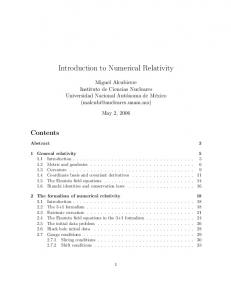
Six-patch results are reported for both second-order and fourth-order differencing of the angular derivatives. In all cases, the fine grid has u = 0.0125 and the coarse grid has u = 0.025. Runs are performed for two complete periods, i.e. starting at u = 0 and ending at u = 4π . Results are reported for the errors of the quantities shown using the L2 (rootmean-square) norm, evaluated at the time shown, averaged over all non-ghost grid-points over the whole sphere and between the inner boundary and future null infinity. The norm of the error in the news is averaged over the whole sphere at future null infinity. Given a quantity , the error ε and the associated convergence factor C are defined as εcoarse C= . (37) ε = numeric − analytic , εfine Thus [36], C = 2 corresponds to first-order, and C = 4 to second-order convergence. As discussed in the introduction, we expect the code to exhibit second-order convergence (C = 4) in the limit of infinite resolution, even when using fourth-order accurate angular derivatives. Figure 2 shows the error norms ε(t) for the metric quantity J , and for the Bondi news N, plotted against time in the case = 2. Each panel of the figure plots ε(t) for the three schemes stereographic, six-patch second order, and six-patch fourth order; and in each case, we plot 4 · ε(t)/4 at fine resolution (points), and ε(t) at coarse resolution (solid line), so that

S336

C Reisswig et al Table 1. This table shows the error norm ε for the low resolution runs, and the convergence factor C, both averaged over space and time, for each version of the code and for each of five diagnostic quantities: the metric variable J , the news function N, and the constraints R00 , R01 and R0A . Quantity

Stereographic


= 2 test data Six-patch, second order

Six-patch, fourth order

C(J ) ε(J ) C(N ) ε(N ) C(R00 ) ε(R00 ) C(R01 ) ε(R01 ) C(R0A ) ε(R0A )

3.8456 3.3039 × 10−9 3.3119 2.2785 × 10−8 1.2487 3.1942 × 10−9 3.5560 3.9214 × 10−11 3.4285 5.2549 × 10−9

3.8286 1.5491 × 10−9 3.9642 1.0913 × 10−8 1.5000 2.8779 × 10−9 3.5936 1.6988 × 10−11 1.7558 6.6397 × 10−9

3.9112 6.9157 × 10−11 3.5528 8.4414 × 10−10 2.0319 5.7668 × 10−10 3.1296 2.7331 × 10−12 2.0043 2.1543 × 10−9

C(J ) ε(J ) C(N ) ε(N ) C(R00 ) ε(R00 ) C(R01 ) ε(R01 ) C(R0A ) ε(R0A )

3.9783 4.6461 × 10−9 2.1201 4.9174 × 10−8 1.2743 7.2594 × 10−9 3.5144 1.3262 × 10−10 3.4326 9.0299 × 10−9


= 3 test data 3.9106 3.2784 × 10−9 3.9134 2.8182 × 10−8 1.7963 4.5824 × 10−9 3.5383 7.5501 × 10−11 1.9510 1.0076 × 10−8

4.0777 1.3677 × 10−10 3.6262 1.7996 × 10−9 2.0330 1.1744 × 10−9 3.3824 6.0924 × 10−12 2.0156 2.9654 × 10−9

for second-order convergence the points and solid line coincide. Table 1 gives the error norm ε (coarse resolution) and the convergence rate C, in both cases averaged over the whole run, for the quantities indicated. It is clear that all schemes give (approximate) second-order convergence of the metric quantity J . However, the news and the constraints (all of which contain second derivatives of metric quantities) exhibited, in some cases, degradation of the order of convergence. Referring to the plot of the news N in figure 2, we see that the six-patch schemes were approximately second-order convergent throughout the run, but that the stereographic scheme exhibited convergence degradation that is periodic in time (Although not shown in the figure, the convergence rate is at all times better than first order). The analytic solution has period 2π , and it is interesting that degradation peaks when the analytic solution is zero. We should also mention that this type of behaviour has shown up in previous performed runs of the stereographic code and may be related to high-frequency error modes coming from angular patch interfaces or corners. The convergence rates of the constraints appear problematic. However, the fact that the convergence rates of R0A (stereographic case) and of R01 (all cases) are nearly second order is important. This implies that the problem is not due either to (a) a simple mis-coding of the finite difference representation of derivatives, or to (b) the expressions generated by the computer algebra. This issue will require further investigation in order to be able to use constraint violation as a reliable indicator of code accuracy. The comparative behaviour of the error norm is particularly interesting. On average, the error norm of second-order six patch was smaller than that of stereographic by a factor of

Characteristic evolutions in numerical relativity using six angular patches

(a)

S337 stereographic 6-patch (2nd order angular FD) 6-patch (4 t h order angular FD)

(b)

-8

10 -9

10

-9

10

-10

||ε(J)||

||ε(N))||

10

-10

10

-11

10

-12

10

-11

0

π

2π t

3π

4π 0

π

2π t

3π

4π

10

Figure 2. This figure shows an example of the convergence and accuracy of the various versions of the code. Part (a) shows results for the metric variable J , while part (b) shows results for the news function N; the same key applies to both parts. In all cases, the solid line shows the coarse resolution results, while the points show the fine resolution results multiplied by 4.

order 2 (although there were cases in which the error was slightly larger). However, the fourth-order six-patch scheme exhibited a dramatic reduction in the error norm, by a factor of up to 47 compared to that of the stereographic case. Although we used the full nonlinear version of the code, we were not able to test nonlinear effects because the analytic solution against which we measure the error is valid only in a linearized regime. Even so, it is expected that the improvement in accuracy associated with the six-patch fourth-order scheme, carries over to the nonlinear regime. The PITT null code in the stereographic version is also capable of evolving non-vacuum spacetimes. Here, we have implemented and tested the six-patch code only for the case of vacuum. Since the ghost-zone scheme used in the six-patch system is known to be able to handle hydrodynamical shocks [37], we expect no problems in extending this method to non-vacuum spacetimes.

6. Conclusion We have implemented a version of the characteristic numerical relativity code that coordinatises the sphere by means of six angular patches. Further, the six-patch code has been implemented for both second-order and fourth-order accurate finite differencing of angular derivatives. We compared the errors and rates of convergence in the various versions of the code, using exact solutions of the linearized Einstein equations as a testbed. This was done for the cases = 2 and = 3, and with several different indicators. In general, the error norm of second-order six patch was smaller than that of stereographic; and the error norm of the fourth-order six-patch scheme was much smaller, by a factor of up to 47, compared to that of the stereographic case. Thus, we expect the six-patch characteristic code, in particular the version that uses fourth-order accurate angular finite differencing, to give significantly better performance than the stereographic version.

S338

C Reisswig et al

Acknowledgments NTB and CWL thank Max-Planck-Institut f¨ur Gravitationsphysik, Albert-Einstein-Institut, for hospitality; and BS and CR thank the University of South Africa for hospitality. The work was supported in part by the National Research Foundation, South Africa, under Grant number 2053724, and by SFB-TR7 ‘Gravitationswellenastronomie’ of the German DFG. JT thanks the Alexander von Humboldt foundation for financial support.

References [1] Bondi H, van der Burg M G J and Metzner A W K 1962 Gravitational waves in general relativity VII. Waves from axi-symmetric isolated systems Proc. R. Soc. A 269 21–52 [2] Sachs R K 1962 Gravitational waves in general relativity VIII. Waves in asymptotically flat space-time Proc. R. Soc. A 270 103–26 [3] Bishop N T, G´omez R, Lehner L, Maharaj M and Winicour J 1997 High-powered gravitational news Phys. Rev. D 56 6298–309 [4] G´omez R 2001 Gravitational waveforms with controlled accuracy Phys. Rev. D 64 024007 [5] Bishop N T, G´omez R, Lehner L and Winicour J 1996 Cauchy-characteristic extraction in numerical relativity Phys. Rev. D 54 6153–65 [6] Bishop N T, G´omez R, Lehner L, Maharaj M and Winicour J 1999 Incorporation of matter into characteristic numerical relativity Phys. Rev. D 60 024005 [7] Bishop N T, G´omez R, Husa S, Lehner L and Winicour J 2003 A numerical relativistic model of a massive particle in orbit near a Schwarzschild black hole Phys. Rev. D 68 084015 [8] G´omez R, Husa S, Lehner L and Winicour J 2002 Gravitational waves from a fissioning white hole Phys. Rev. D 66 064019 [9] Bishop N T, Clarke C and d’Inverno R 1990 Numerical relativity on a transputer array Class. Quantum Grav. 7 L23–7 [10] dInverno R A and Vickers J A 1997 Combining Cauchy and characteristic codes: IV. The characteristic field equations in axial symmetry Phys. Rev. D 56 772–84 [11] dInverno R A, Dubal M R and Sarkies E A 2000 Cauchy-characteristic matching for a family of cylindrical solutions possessing both gravitational degrees of freedom Class. Quantum Grav. 17 3157–70 [12] Papadopoulos P and Font J A 1999 Relativistic hydrodynamics on spacelike and null surfaces: formalism and computations of spherically symmetric spacetimes Phys. Rev. D 61 024015 [13] Siebel F, Font J A, Mueller E and Papadopoulos P 2003 Axisymmetric core collapse simulations using characteristic numerical relativity Phys. Rev. D 67 124018 [14] Siebel F and Font J A 2001 Scalar field induced oscillations of relativistic stars and gravitational collapse Phys. Rev. D 65 024021 [15] Bartnik R A and Norton A H 1999 Einstein equations in the null quasi-spherical gauge: III. Numerical algorithms Preprint gr-qc/9904045 [16] Bishop N T, G´omez R, Lehner L, Maharaj M and Winicour J 2005 Characteristic initial data for a star orbiting a black hole Phys. Rev. D 72 024002 [17] Babiuc M, Szilagyi B, Hawke I and Zlochower Y 2005 Gravitational wave extraction based on Cauchycharacteristic extraction and characteristic evolution Class. Quantum Grav. 22 5089–108 [18] G´omez R, Lehner L, Marsa R L and Winicour J 1998 Moving black holes in 3D Phys. Rev. D 57 4778–88 [19] Zlochower Y, G´omez R, Husa S, Lehner L and Winicour J 2003 Mode coupling in the nonlinear response of black holes Phys. Rev. D 68 084014 [20] Thornburg J 2004 Black hole excision with multiple grid patches Class. Quantum Grav. 21 3665–91 [21] Calabrese G and Neilsen D 2004 Spherical excision for moving black holes and summation by parts for axisymmetric systems Phys. Rev. D 69 044020 [22] Calabrese G and Neilsen D 2005 Excising a boosted rotating black hole with overlapping grids Phys. Rev. D 71 124027 [23] Anderson M W 2004 Constrained evolution in numerical relativity PhD Thesis, The University of Texas at Austin, Austin, Texas, USA [24] Lehner L, Reula O and Tiglio M 2005 Multi-block simulations in general relativity: high order discretizations, numerical stability, and applications Class. Quantum Grav. 22 S283-322

Characteristic evolutions in numerical relativity using six angular patches

S339

[25] Diener P, Dorband E N, Schnetter E and Tiglio M 2005 New, efficient, and accurate high order derivative and dissipation operators satisfying summation by parts, and applications in three-dimensional multi-block evolutions Preprint gr-qc/0512001 [26] Schnetter E, Diener P, Dorband N and Tiglio M 2006 A multi-block infrastructure for three-dimensional time-dependent numerical relativity Class. Quantum Grav. 23 S553–78 [27] Dorband E N, Berti E, Diener P, Schnetter E and Tiglio M 2006 A numerical study of the quasinormal mode excitation of Kerr black holes Phys. Rev. D 74 084028 [28] Bishop N T 2005 Linearized solutions of the Einstein equations within a Bondi-Sachs framework, and implications for boundary conditions in numerical simulations Class. Quantum Grav. 22 2393–406 [29] Goodale T, Allen G, Lanfermann G, Mass´o J, Radke T, Seidel E and Shalf J 2003 The Cactus framework and toolkit: design and applications VECPAR’2002: Vector and Parallel Processing—5th Int. Conf. (Lecture Notes in Computer Science) (Berlin: Springer) [30] Schnetter E, Hawley S H and Hawke I 2004 Evolutions in 3D numerical relativity using fixed mesh refinement Class. Quantum Grav. 21 1465–88 [31] Isaacson R, Welling J and Winicour J 1983 Null cone computation of gravitational radiation J. Math. Phys. 24 1824 [32] G´omez R, Lehner L, Papadopoulos P and Winicour J 1997 The eth formalism in numerical relativity Class. Quantum Grav. 14 977–90 [33] Newman E T and Penrose R 1966 Note on the Bondi-Metzner-Sachs group J. Math. Phys. 7 863–70 [34] Goldberg J N, MacFarlane A J, Newman E T, Rohrlich F and Sudarshan E C G 1967 Spin-s spherical harmonics and
J. Math. Phys. 8 2155–61 [35] Fornberg B 1988 Generation of finite difference formulas on arbitrarily spaced grids Math. Comput. 51 699–706 [36] Choptuik M W 1991 Consistency of finite-difference solutions to Einstein’s equations Phys. Rev. D 44 3124–35 [37] Hawke I 2005 personal communication to Jonathan Thornburg