JOURNAL OF APPLIED PHYSICS
VOLUME 85, NUMBER 9
1 MAY 1999
Characterizing interactions in fine magnetic particle systems using first order reversal curves Christopher R. Pikea) Department of Geology, University of California, Davis, California 95616
Andrew P. Roberts Department of Oceanography, University of Southampton, Southampton Oceanography Centre, European Way, Southampton SO14 3ZH, United Kingdom
Kenneth L. Verosub Department of Geology, University of California, Davis, California 95616
~Received 1 June 1998; accepted for publication 1 February 1999! We demonstrate a powerful and practical method of characterizing interactions in fine magnetic particle systems utilizing a class of hysteresis curves known as first order reversal curves. This method is tested on samples of highly dispersed magnetic particles, where it leads to a more detailed understanding of interactions than has previously been possible. In a quantitative comparison between this method and the d M method, which is based on the Wohlfarth relation, our method provides a more precise measure of the strength of the interactions. Our method also has the advantage that it can be used to decouple the effects of the mean interaction field from the effects of local interaction field variance. © 1999 American Institute of Physics. @S0021-8979~99!08309-7#
I. INTRODUCTION
field. This field is ramped down to a reversal field H a . The FORC consists of a measurement of the magnetization as the field is then increased from H a back up to saturation. The magnetization at applied field H b on the FORC with reversal point H a is denoted by M (H a ,H b ), where H b >H a . A FORC distribution is defined as the mixed second derivative:
Magnetic interactions between particles are a major determinant of noise levels in magnetic recording media. The conventional methods1–3 of characterizing magnetic interactions utilize isothermal remanent magnetization ~IRM! and dc demagnetization remanence ~DCD! curves, and are based on the Wohlfarth4 relation. The most important among these methods is the d M method.5,6 In this paper, an alternative approach is described which employs first order reversal curves ~FORCs!.7 A typical set of FORCs is shown in Fig. 1. The structure present in this set of curves is not readily apparent, but it can be emphasized with a mixed second derivative as described more formally below. In this fashion, the FORCs of Fig. 1 can be transformed into the contour plot of Fig. 2, which we will refer to as a FORC diagram. ~There are obvious similarities between a FORC diagram and a Preisach diagram,8 but there are also important distinctions, which we discuss in Appendix A.! We have developed a practical technique for measuring and calculating accurate FORC diagrams. This technique requires thousands of data points, and, until recently, would have been impractical. However, with the advent of a commercially available, automated alternating field gradient magnetometer,9 the acquisition of a FORC diagram is a straightforward task, requiring only a couple of hours for data collection and analysis.
r ~ H a ,H b ! [2
~1!
where this is well defined only for H b .H a . When a FORC distribution is plotted, it is convenient to change coordinates from $ H a ,H b % to $ H c [(H b 2H a )/2, H u [(H a 1H b )/2% . A FORC diagram is a contour plot of a FORC distribution with H c and H u on the horizontal and vertical axes, respectively. Since H b .H a , then H c .0, and a FORC diagram is confined to the right side half plane. As shown below, when the basic Preisach model is used, H c is equivalent to a particle coercivity and H u to a local interaction field. To evaluate a FORC diagram, first the boundaries of the desired diagram in the H c , H u plane are selected. The reversal field of the first FORC, H a1 , is calculated from the coordinates of the upper left corner of the diagram @i.e., H a 5(H u 2H c )#; the reversal field of the last FORC, H aN , is calculated from the bottom right corner; and N FORCs are measured with evenly spaced reversal fields between and including H a1 and H aN . The data points on each individual FORC are measured with this same field spacing. The same averaging time is used in the measurement of every data point. In choosing N, the number of FORCs to be measured, there is a tradeoff between the resolution of the FORC diagram and data acquisition time. We have found that N599
II. EVALUATION OF A FORC DIAGRAM
The measurement of a FORC, as shown in Fig. 3, begins with the saturation of the sample by a large positive applied a!
Electronic mail:
[email protected]
0021-8979/99/85(9)/6660/8/$15.00
] 2 M ~ H a ,H b ! , ] H a] H b
6660
© 1999 American Institute of Physics
Downloaded 24 Dec 2002 to 152.78.0.29. Redistribution subject to AIP license or copyright, see http://ojps.aip.org/japo/japcr.jsp
J. Appl. Phys., Vol. 85, No. 9, 1 May 1999
FIG. 1. A set of first order reversal curves ~FORCs! for a piece of a typical floppy magnetic recording disk.
yields a reasonable resolution in an acquisition time between 1 and 2 h. To calculate r (H a ,H b ) we use consecutive data points from consecutive reversal curves in an array such as that shown in Fig. 4. We fit the magnetization at these points with a polynomial surface of the form: a 1 1a 2 H a 1a 3 H 2a 1a 4 H b 1a 5 H 2b 1a 6 H a H b ; then 2a 6 is taken as the value of r (H a ,H b ) at the center of the array. The number of data points contained in this array is (2 * SF11) 2 , where SF is referred to as the ‘‘smoothing factor’’ and can be set between 3 for a well-behaved sample and 10 for a noisy sample. Numerical effects inevitably smooth out somewhat the features of a FORC distribution; the degree of smoothing increases with the value of SF. In practice, one tries to use the smallest value of SF possible, while keeping noise on a FORC diagram to acceptable levels. The FORC diagrams in this paper were evaluated with SF53. III. EXPERIMENTAL RESULTS
FORC distributions were measured for a sample of magnetic recording material from a typical floppy disk and for samples of highly dispersed, single domain magnetic particles prepared by Eastman Kodak Company Research Laboratories at four concentrations of: 1.5%, 3%, 6% and 9% of magnetic material by mass. As far as it was possible to control, the concentration of particles and, hence, the proximity of particles to each other, was the only parameter allowed to vary between samples. FORC diagrams for the floppy disk material and for a 1.5% Kodak sample are shown in Figs. 2 and 5, respectively. The averaging time spend at each data point was 0.4 s. To
FIG. 2. A FORC diagram for a floppy disk sample. Calculated from 99 FORCs of which the data in Fig. 1 are a subset.
Pike, Roberts, and Verosub
6661
FIG. 3. Definition of a FORC. The measurement of a FORC begins with the saturation of the sample by a large positive field. This field is ramped down to a reversal field H a . The FORC consists of a measurement of the magnetization as the field is then increased from H a back up to saturation. The magnetization at H b on the FORC with reversal point H a is denoted by M (H a ,H b ).
emphasize the differences between the Kodak samples, we also acquired FORC diagrams for a smaller region of the FORC plane, as shown in Fig. 6 for a 1.5% and 9% sample. Each FORC diagram required a separate measurement of 99 FORCs. Since the diagrams in Fig. 6 have a smaller size, the 99 FORCs used to evaluate them had a smaller field spacing ~1 mT! than those used to calculate Fig. 5 ~2 mT!, which provides for a greater resolution. IV. THEORETICAL MODELS
A FORC diagram contains a large amount of information, but this information is of little use if it cannot be correctly interpreted. To facilitate our interpretation of these diagrams, we can study the FORC diagrams associated with theoretical models. This will permit us to assign interpretations to the features we see on experimental diagrams. Therefore, below we calculate FORC distributions for some simple theoretical models. A. Noninteracting single domain particles
Our first model consists of a collection of noninteracting single domain, particles. The magnetic behavior of an individual single domain particle can, to a good approximation, be represented as the sum of a reversible component and a square hysteresis loop. In the noninteracting case, the reversible component will vanish when the second derivative in Eq. ~1! is taken and can be ignored. The half width of the square loop is termed a particle’s switching field. A collection of particles can be represented by a distribution of switching fields f (H sw ;H sw.0), where * `0 dx f (x)51. To
FIG. 4. A subset of seven consecutive FORCs from Fig. 1. The circled points are a 737 array of data points evenly spaced in H a and H b .
Downloaded 24 Dec 2002 to 152.78.0.29. Redistribution subject to AIP license or copyright, see http://ojps.aip.org/japo/japcr.jsp
6662
J. Appl. Phys., Vol. 85, No. 9, 1 May 1999
Pike, Roberts, and Verosub
FIG. 5. FORC diagram for a 1.5% Kodak sample. Field spacing: 3 mT.
calculate the magnetization on a FORC, we start with a saturating positive applied field, so all the particles have a positive orientation. At H a , particles with switching fields in the range 0