choice of the Ewald splitting parameter was performed in. Capolino et al. ... For the 2-D array with lattice vectors s1, s2 (see Figure 3), the parameters are defined ...
RADIO SCIENCE, VOL. 43, RS6S01, doi:10.1029/2007RS003820, 2008
Choosing splitting parameters and summation limits in the numerical evaluation of 1-D and 2-D periodic Green’s functions using the Ewald method Ferhat T. Celepcikay,1 Donald R. Wilton,1 David R. Jackson,1 and Filippo Capolino2 Received 26 December 2007; revised 14 April 2008; accepted 5 May 2008; published 30 September 2008.
[1] Accurate and efficient computation of periodic free-space Green’s functions using the
Ewald method is considered for three cases: a 1-D array of line sources, a 1-D array of point sources, and a 2-D array of point sources. A limitation on the numerical accuracy when using the ‘‘optimum’’ E parameter (which gives optimum asymptotic convergence) at high frequency is discussed. A ‘‘best’’ E parameter is then derived to overcome these limitations. This choice allows for the fastest convergence while maintaining a specific level of accuracy (loss of significant figures) in the final result. Formulas for the number of terms needed for convergence are also derived for both the spectral and the spatial series that appear in the Ewald method, and these are found to be accurate in almost all cases. Citation: Celepcikay, F. T., D. R. Wilton, D. R. Jackson, and F. Capolino (2008), Choosing splitting parameters and summation limits in the numerical evaluation of 1-D and 2-D periodic Green’s functions using the Ewald method, Radio Sci., 43, RS6S01, doi:10.1029/2007RS003820.
1. Introduction [2] In applying numerical full wave methods like the Method of Moments (MoM) or Boundary Integral Equations (BIE) to periodic structures involving conducting or dielectric electromagnetic scatterers, fast and accurate means for evaluating the free-space periodic Green’s function (FSPGF) are often needed. This type of Green’s function arises in a wide variety of applications, ranging from microwaves to optics, to the study of metamaterials and nanostructures. The Ewald method is one of the fastest methods for calculating the FSPGF. In the Ewald method, the FSPGF is expressed as the sum of a ‘‘modified spectral’’ and a ‘‘modified spatial’’ series. The terms of both series possess Gaussian decay, leading to an overall series representation that exhibits a very rapid convergence rate. The convergence rate is optimum when the ‘‘optimum’’ value of the Ewald splitting parameter is used [Jordan et al., 1986], denoted here as Eopt. (For some applications, such as when using a periodic Green’s function in a MoM 1 Department of Electrical and Computer Engineering, University of Houston, Houston, Texas, USA. 2 Department of Electrical Engineering and Computer Science, University of California, Irvine, California, USA.
Copyright 2008 by the American Geophysical Union. 0048-6604/08/2007RS003820
solution with full-domain basis functions, one may not wish to have a balanced convergence between the two series, as explained in Mathis and Peterson [1996] and Mathis and Peterson [1998]. However, when using subdomain basis functions and performing the integrations over the basis and testing functions in the spatial domain, the objective is to minimize the computation time of the periodic Green’s function, and this is accomplished by using Eopt. In this case the singular integrals involved in evaluating the matrix elements can be handled by specially designed numerical quadrature rules [Khayat and Wilton, 2005].) [3] However, the numerical accuracy of the Ewald method degrades very quickly [Kustepeli and Martin, 2000] with increasing frequency (i.e., when the periodicity becomes large relative to a wavelength). This is due to a catastrophic loss of significant figures in combining the contributions of the two series, wherein the leading terms (and to a lesser extent, other nearby terms) in each series become very large but nearly equal and opposite in sign. [4] The method proposed and studied here limits the size of the largest terms in the series relative to that of the total Green’s function by modifying the value of the splitting parameter E to avoid undue loss of accuracy. Increasing the E parameter limits the size of the largest terms in both series at the expense of decreasing the convergence rate. Hence, there is a tradeoff between the size of the largest term allowed, which
RS6S01
1 of 11
RS6S01
CELEPCIKAY ET AL.: NUMERICAL EVALUATION OF EWALD METHOD
determines the number of significant figures lost, and the series convergence rate. A value EL of the Ewald splitting parameter is then obtained based on the number of significant figures L that may be lost. This ‘‘best’’ value, EL, then yields the fastest convergence of the Ewald series while limiting the loss of significant figures to the user-defined value L. [5] A preliminary and intuitive analysis for the ‘‘best’’ choice of the Ewald splitting parameter was performed in Capolino et al. [2005] for the case of 1-D array of line sources, and in Capolino et al. [2007] for the case of a 1-D array of point sources. The case of a 2D-array of point sources has been treated in detail in Oroskar et al. [2006]. Here we extend the analysis of the last paper to the two other cases, and provide a unified formalism for the choice of the Ewald splitting parameter and the summation limits that is valid for all three cases.
2. Spectral, Spatial, and Ewald Green’s Function Representations [6] Three different FSPGF cases are considered: a 1-D array of line sources with interelement period d, a 2-D array of point sources on a general skewed lattice, and a 1-D array of point sources with interelement spacing d. The geometries are depicted along with relevant coordinate systems and geometrical definitions in Figures 1, 2, and 3, respectively. An interelement phase shift along the array direction(s) is assumed. Both spatial and spectral representations of each Green’s function exist in the general form Gðr; r0 Þ ¼ 8 1 X > > > Gm > > < m¼�1 1 1 > X X > > > Gm;n > : m¼�1 n¼�1
¼
1 X
~ p; G
1 � D array
whereas those of the spectral representations are 0
�jkxp ð x�x Þ ~p ¼ 1 e G e�jkzp Dz ; 1 � D array of line sources d 2jkzp � � ~ p ¼ 1 e�jkxp ð x�x0 Þ H ð2Þ krp r ; G 0 4jd
1 � D array of point sources �jktpq � ðr � r0 Þ �jkzpq Dz ~ p;q ¼ 1 e G e ; A 2jkzpq
2 � D array of point sources ð3Þ
where Dz � |z � z0| and an ejwt time dependence is assumed and suppressed. In the above, (x, y, z) and (x0, y0, z0) denote the observation and reference-element source points, respectively. For the 1-D cases, the periodicity is along x with a period of d (see Figures 1 and 2), and 2pp ; d qffiffiffiffiffiffiffiffiffiffiffiffiffiffiffiffi 2 kzp ¼ krp ¼ k 2 � kxp qffiffiffiffiffiffiffiffiffiffiffiffiffiffiffiffiffiffiffiffiffiffiffiffiffiffiffiffiffiffiffiffiffiffiffiffiffiffiffiffiffiffiffiffiffiffiffiffiffi Rm ¼ ð z � z0 Þ2 þð x � x0 � md Þ2 kxp ¼ kx0 þ
ð1 � D array of line sourcesÞ; qffiffiffiffiffiffiffiffiffiffiffiffiffiffiffiffiffiffiffiffiffiffiffiffiffiffiffiffiffiffiffiffiffiffiffiffiffiffiffiffiffiffiffiffiffiffiffiffiffiffiffiffiffiffiffiffiffiffiffiffiffiffiffiffiffiffiffiffiffiffi Rm ¼ ð z � z0 Þ2 þð y � y0 Þ2 þð x � x0 � md Þ2 ð1 � D array of point sourcesÞ; qffiffiffiffiffiffiffiffiffiffiffiffiffiffiffiffiffiffiffiffiffiffiffiffiffiffiffiffiffiffiffiffiffiffiffiffiffiffi r ¼ ð y � y0 Þ2 þð z � z0 Þ2
p¼�1
¼
1 1 X X
ð1 � D array of point sourcesÞ: ~ p;q ; 2 � D array G
p¼�1 q¼�1
ð1Þ
For the 2-D array with lattice vectors s1, s2 (see Figure 3), the parameters are defined as r ¼ x^x þ y^y; r0 ¼ x0 ^x þ y0 ^y; rmn ¼ ms1 þ ns2 ; qffiffiffiffiffiffiffiffiffiffiffiffiffiffiffiffiffiffiffiffiffiffiffiffiffiffiffiffiffiffiffiffiffiffiffiffiffiffiffiffiffiffiffiffiffiffiffiffiffiffiffi Rmn ¼ ð z � z0 Þ2 þjr � r0 � rmn j2 ;
where the terms of the spatial representations are 1 ð2Þ H ðkRm Þ; 1 � D array of line sources 4j 0 e�jkRm Gm ¼ e�jkx0 md ; 1 � D array of point sources 4pRm e�jkRmn Gm;n ¼ e�jkt00 �rmn ; 2 � D array of point sources 4pRmn ð2Þ Gm ¼ e�jkx0 md
RS6S01
kt00 ¼ kx0 ^x þ ky0 ^y; 2ppðs2 � ^zÞ 2qpð^z � s1 Þ þ ; ktpq ¼ kt00 þ A A qffiffiffiffiffiffiffiffiffiffiffiffiffiffiffiffiffiffiffiffiffiffiffiffiffiffiffiffi kzpq ¼ k 2 � ktpq � ktpq ; A ¼ ^z � ðs1 � s2 Þ:
The transverse phasing wave vector kt00 = ^ xk sin q0 cos f0 + ^ yk sin q0 sin f0 defines the interelement phasing for the 2-D
2 of 11
RS6S01
CELEPCIKAY ET AL.: NUMERICAL EVALUATION OF EWALD METHOD
Figure 1. One-dimensional array of line sources parallel to the y-axis, periodic with period d along the x-axis. The observation point and reference line source are shown.
RS6S01
Figure 3. Two-dimensional array of point sources parallel to the xy-plane, periodic with lattice vectors s1 and s2. The observation point and reference source point are shown.
array in terms of the propagation angles q0, f0 of the (0, 0) Floquet mode. For 1-D arrays, this quantity becomes the scalar phasing kx0 = k cos q0, where q0 is measured with respect to the x-axis. Physically the FSPGF is the time[8] When employing the Ewald method for the evalharmonic scalar potential produced by the associated array of uation of the FSPGF, the Green’s function is expressed as phased sources. a sum of two series [Ewald, 1921] of the form 8 1 1 X X > > E ~ E; > G þ 1 � D array G > m p < m¼�1 p¼�1 0 ð4Þ Gðr; r Þ ¼ 1 1 1 1 X X X X > > E ~ E ; 2 � D array: > G þ G > m;n p;q : m¼�1 n¼�1
[7] For a lossless medium the square root for the wave numbers krp and kzpq is that which gives a positive real number or a negative imaginary number, corresponding to waves that propagate outward or decay away from the sources, respectively. For a lossy medium the wave numbers are complex and it suffices to require the imaginary part of the wave numbers to be negative. Henceforth, it will be assumed that the medium is lossless, but the formulas can be extended to the lossy case.
p¼�1 q¼�1
The terms that appear in the three different cases may be found in Capolino et al. [2005], Capolino et al. [2007], and Oroskar et al. [2006], for the 1-D array of line sources, the 1-D array of point sources, and the 2-D array of point sources, respectively. Summarizing, the terms of the modified spatial representations are " # �2q 1
X � � 1 k 1 e�jkx0 md Eqþ1 R2m E2 GEm ¼ 4p 2E q! q¼0
GEm
1 � D array of line sources;
� 1e k �jkRm ¼ e erfc Rm E � j 2 4pRm 2E
�� k þ ejkRm erfc Rm E þ j 2E
GEm;n
�jkx0 md
�
1 � D array of point sources; �
� 1e k �jkRmn ¼ e erfc Rmn E � j 2 4pRmn 2E
�� k þ ejkRmn erfc Rmn E þ j 2E �jkt00 �rmn
2 � D array of point sources; ð5Þ
Figure 2. One-dimensional array of point sources, periodic with period d along the x-axis. The observation point and reference source point are shown.
where erfc(z) is the complementary error function and Eq(z) denotes the exponential integral function of order
3 of 11
CELEPCIKAY ET AL.: NUMERICAL EVALUATION OF EWALD METHOD
RS6S01
RS6S01
Table 1. Definition of Parameters Appearing in the Iterative Equation for Determining EL
1-D array of line sources
Spatial
Spectral 1-D array of point sources
Spatial Spectral
2-D array of point sources
Spatial Spectral
z k
K
10 4p|G |
2Espatial kz0 2Espectral k 2Espatial kr0 2Espectral k 2Espatial kz00 2Espectral
kz0 Dz 2 kR0 2 kr0 r 2 kR00 2 kz00 Dz 2
pffiffiffi 10L2 pkz0d|Gest|
q. The terms of the modified spectral representations are
� 0 � jkzp 1 e�jkxp ð x�x Þ �jkzp Dz E ~ � DzE e erfc Gp ¼ 2d 2jkzp 2E
�� jkzp þ ejkzp Dz erfc þ DzE 2E 1 � D array of line sources; " !# 2 q 1 X �krp 1 ð �1 Þ 0 E 2q �jk ð x�x Þ xp ~ ¼ G e Eqþ1 ð rEÞ p 4pd q! 4E 2 q¼0
~E G p;q
F(z )
c1
kR0 2
1 � D array of point sources; �
� jkzpq 1 e � DzE ¼ e�jkzpq Dz erfc 2A 2jkzpq 2E
�� jkzpq þ ejkzpq Dz erfc þ DzE 2E �jktpq �ðr�r0 Þ
2 � D array of point sources: ð6Þ
For the 1-D array of point sources, the exponential integral function that appears may have a negative argument, depending on the frequency. In this case the argument is interpreted as being infinitesimally above the branch cut of the exponential integral function on the negative real axis, corresponding to an infinitesimal amount of loss.
3. Splitting Parameter (E) [9] In equations (5) and (6) the spatial and spectral series both involve a ‘‘splitting’’ parameter E. The ‘‘optimum value’’ Eopt for the splitting parameter [Jordan et al., 1986] balances the asymptotic rate of convergence of the
L
est
c1z 2
c1 z
3
10L4(p)2 R0|Gest|
c1
�
� z �� K
10L4pd|Gest|
pffiffiffi 10L2 pkz00A|Gest|
� 2
�
2
�
z 2 þ Kz 2
c1z 2
3
10L4(p)2 R00|Gest|
2
z 2 þ Kz 2
c1
� � �� K
c1 z
�
z 2 þ Kz 2 2
z 2 þ Kz 2
�
spatial and spectral series, and consequently minimizes the overall number of terms needed to calculate the total FSPGF. The optimum value is found to be 8 pffiffiffi p > > < ; 1 � D array d ð7Þ Eopt ¼ rffiffiffi p > > : ; 2 � D array: A However, numerical difficulties are encountered when the lattice separations (periods) become large relative to a wavelength. This was first discovered in Kustepeli and Martin [2000], and subsequently also discussed in Capolino et al. [2005], Oroskar et al. [2006], and Capolino et al. [2007]. This happens because, for large arguments, both the complementary error function and the exponential integrals contribute terms of the form exp[(k/(2E))2] that produce extremely large initial terms (and to a lesser extent, large nearby terms) in both the spatial and the spectral series. The resulting series then each converge to very large, but nearly equal and oppositely signed values, resulting in a total sum of moderate value but with a catastrophic loss of significant figures when the two series are combined. Exponential overflow is another potential concern as well, due to the large initial values in each series. [10] To circumvent the problem, it is desirable to limit the size of the largest terms of each series by choosing an E value larger than the ‘‘optimum’’ value, which reduces the maximum values of both the complementary error function and the exponential integrals. As a result, one avoids loss of accuracy in adding the two series, and a more accurate result for the total Green’s function is obtained [Kustepeli, and Martin, 2000] at the expense of slower convergence.
4 of 11
RS6S01
CELEPCIKAY ET AL.: NUMERICAL EVALUATION OF EWALD METHOD
[11] In the following sections, a recipe for finding the best choice for E, called EL, that achieves the fastest convergence under the constraint of limiting the loss of significant figures to L digits, is obtained for a general source and observation point, for all three cases.
4. Choice of the Splitting Parameter [12] The strategy is to limit the size of the largest terms relative to the value of the total Green’s function, with the largest terms in each series being the initial (0) or (0, 0) terms in 1-D or 2-D, respectively. The value of E = EL is obtained by enforcing the following conditions: � � � � 9 � ~ E� � E� �G0 �; G0 ; 1 � D array = � � � � < a 10L jGest j ð8Þ �~E � � E � �G0;0 �; �G0;0 �; 2 � D array ;
RS6S01
In (9), the indices p, q, m, n that produce the smallest values for Rm, Rmn, krp, kzp, and kzpq must be determined; although this may be done analytically, it is also very easy to find these values from a simple numerical search. [13] To proceed with the derivation of EL, we replace the terms on the left hand side of (8) by their highfrequency asymptotic estimates. The complementary error function terms are estimated by using the asymptotic relation 2
e�z erfcð zÞ � pffiffiffi ; pz
ð10Þ
valid for large arguments. In addition, in (5) and (6) series of exponential integral functions appear. The simplest way to asymptotically evaluate these series is to re-cast them back into their integral forms. The integral forms are equation (15) in Capolino et al. [2007] and equation (11) in Capolino et al. [2005], which are reproduced below: ! 2 r2 Z1 2 1 X �krp e� 4uþðkrp Þ u ð�1Þq 2q du ¼ ð rEÞ Eqþ1 u q! 4E 2 q¼0
where Gest is a closed-form estimate of the FSPGF, and the integer parameter L indicates (roughly) the number of significant figures one is willing to sacrifice in the calculation. For a strict bound, the factor a in (8) should be chosen as 1/2 to ensure that each of the two initial terms in (8) (one from the spatial series and one from the 1=ð2EÞ2 spectral series) contributes no more than half the total ð11Þ error limit. However, it is found in each of the three cases that one of the initial terms (either the spatial one or the spectral one, depending on the case) is significantly � Z1 �R2m s2 þ k 22 1
� � 4s larger than the other, and a factor of a = 1 therefore e 1X k 2q 1 Eqþ1 R2m E 2 : ð12Þ ds ¼ becomes more appropriate, and this is adopted here. It 2 q¼0 2E q! s E suffices to use a rough estimate of the Green’s function on the right-hand side of (8), which may be obtained by examining the most nearly singular terms from both the The integrals that appear in the above identities may be spatial and the spectral series. (This is an improvement asymptotically evaluated for k!1 via integration by over the previous derivations, as in Oroskar et al. [2006], where only the spatial term was used.) This yields the following magnitude estimate for the overall Green’s function: � 8 0�� ð2Þ 1 � > H0 ðkRm Þ� � > 1 > > ; �� �� A; 1 � D array of line sources max@ > > > 4 2 kzp d > > > > > > > > > > � > 0 > ���1 � ð2Þ � < H k r � � rp est jG j max@ 1 ; 0 A; 1 � D array of point sources > > 4pRm 4d > > > > > > > > > > > ! > > > > 1 1 > > ð9Þ ; � � ; 2 � D array of point sources: : max 4pRmn 2A�kzpq �
5 of 11
CELEPCIKAY ET AL.: NUMERICAL EVALUATION OF EWALD METHOD
RS6S01
parts [Felsen and Marcuvitz, 1994; Bleistein and Handelsman, 1986] (see case 1a and case 2a of Appendix A for further details), yielding �kr0 �2 2 2 r2 Z1 e� 4uþðkr0 Þ u e�ðrEÞ þ 2E du � � ð13Þ � �2 u kr0 1=ð2E Þ2
Z1 E
2E
2
2
2
k
ð14Þ
Applying (9) – (14) in (8), as detailed in Oroskar et al. [2006] yields in each case (spectral and spatial) a transcendental equation of the form
�2 K 2 z � ¼ lnð F ðz ÞÞ; ð15Þ z where the constant K and the function F in (15) are defined in Table 1 (in each case the function F contains a factor c1 that is also shown). Solving the quadratic form for z on the left-hand side of (15) puts the equation into the following form that may be efficiently solved iteratively, due to the slow variation of the ln function: vffiffiffiffiffiffiffiffiffiffiffiffiffiffiffiffiffiffiffiffiffiffiffiffiffiffiffiffiffiffiffiffiffiffiffiffiffiffiffiffiffiffiffiffiffiffi qffiffiffiffiffiffiffiffiffiffiffiffiffiffiffiffiffiffiffiffiffiffiffiffiffiffiffi u u iþ ln F ðln F i Þ2 þ4K 2 t z iþ1 ¼ ; ð16Þ 2 where Fi = F(z i). [14] The solution of (15) yields the parameter z, which (see Table 1) is inversely proportional to the desired Ewald parameter E. Two E values, Espectral and Espatial, result from this procedure. To properly bound both series, E should then be chosen as � � EL ¼ max Eopt ; Espectral ; Espatial :
� E �G
The resulting value is the smallest value of E that ensures that the largest term in both the spectral and the spatial series (see equation (8)) is limited in magnitude to avoid losing more than L significant figures when the two series are combined. At low or moderate frequency, where the initial terms of the spectral and spatial series are not large, EL = Eopt since Eopt will be the largest of the three terms in (17).
2
e�ðR0 sÞ þð2sÞ e�ðR0 EÞ þð2EÞ ds � : � k �2 s 2 2E k
RS6S01
ð17Þ
5. Number of Terms Needed for Convergence [15] Having determined the ‘‘best’’ value of the E parameter EL as a function of frequency, the next goal is to determine how many terms should be summed in each series (modified spatial and modified spectral) in (4) to achieve convergence. (One could, of course, check convergence as the series are summed, but we eventually want to select between the Ewald and alternative methods for computing the FSPGF that may be more efficient in some situations; for that an a priori estimate of the number of series terms and their relative computational cost is required.) Recall that a given value of L, the number of significant figures sacrificed in the calculation, has been assumed. For the resulting value of E = EL we must then determine how many terms in each series are needed to guarantee convergence of the Green’s function to S significant figures. A method is developed here to calculate the series index limits ±P, ±Q, ±M, and ±N for the series indices p, q, m, and n, respectively (Q and N only apply for the 2-D geometry). If the accuracy of the arithmetic is limited to T significant figures due to the machine precision (or, more likely in practice, limited by the accuracy of the complementary error function and exponential integrals), the value of S specified should be limited to S < T � L in order to avoid unnecessary computation. [16] Owing to the Gaussian convergence, a rough estimate of the truncation error for both the spectral and spatial series is obtained by using the sum of the largest of the first neglected terms along each principal sum index in the series. Limiting the convergence error in each series to one half of the total, we thus require that 9
� 1 � D array = 1 �S est � < 10 G b ð18Þ j j � ; 2 �; 2 � D array
� � E � � þ �G � �M �1 ; � � � � � � � � E � � � � � � �GM þ1;0 � þ �GE�M �1;0 � þ �GE0;Nþ1 � þ �GE0;�N �1 M þ1
9 � E � � E � �G �; ~ � þ �G ~ >
� 1 � D array = Pþ1 �P�1 1 � � � � � � � � < 10�S jGest j b: �~E � �~E � �~E � �~E � > 2 �GPþ1;0 � þ �G�P�1;0 � þ �G0;Qþ1 � þ �G0;�Q�1 �; 2 � D array ;
6 of 11
ð19Þ
RS6S01
CELEPCIKAY ET AL.: NUMERICAL EVALUATION OF EWALD METHOD
RS6S01
Table 2. Definition of Parameters Appearing in the Summation Limit Equation
1-D array of line sources
Spatial Spectral
x
c2
W
�RmE� �kzp �
0
10-S e�(k/(2E)) |Gest|pb
jEDz
2E 1-D array of point sources
Spatial
�RmE� �krp �
Spectral
�RmnE� �kzpq �
Spatial Spectral
10-S
pffiffiffi pdE|Gest|e�2c b 2 2
3
2
k 2E
10-S (p)2 |Gest|e�2c2b/E
0
10�S e(rE) jGestjpdb
k 2E
10-S (p)2 |Gest|e�2c2b/(2E)
2E 2-D array of point sources
2
jEDz
2
3
10-S
2
pffiffiffi pAE|Gest|e�2c b/2 2 2
2E The error in stopping the summations is approximated in arrays, and the index pairs (m, n) = (M + 1, 0), (0, N + 1) and the above equations as the sum of the two (four) values (p, q) = (P + 1, 0), (0, Q + 1) for the 2-D array. [19] The results for the case of a 1-D line source array are that give the largest contributions to the summed values for 1-D (2-D) arrays. The factor b is introduced to allow 0 ffiffiffiffiffiffiffiffiffiffiffiffiffiffiffiffiffiffiffiffiffiffiffiffiffiffiffiffiffiffiffiffi ffi1 s
�2 for an empirical adjustment of the summation limits. 0 j x � x j 1 x Using b = 1 corresponds to a strict error bound based on M ¼ Int@ þ �ð z � z0 Þ2 A; d d E the assumed asymptotic approximations, and therefore
qffiffiffiffiffiffiffiffiffiffiffiffiffiffiffiffiffiffiffiffiffiffiffiffi� usually represents a worst-case error bound. However, j kx0 j d d factors of b = 2 and b = 4 have been found to work well P ¼ Int þ k 2 þ ð2ExÞ2 : ð22Þ 2p 2p for the 1-D and 2-D cases, respectively. If we assume that the contributions of the positively indexed terms on the LHS of inequalities (18) and (19) are dominant, the choice of the limits amounts to choosing M, N, P, Q such that
� � E � �� E �� �G �; �G ~ � < 10�S jGest j 1 b; 1 � D array M þ1 Pþ1 4 ð20Þ
� � � � � � � � � 1 � E � � � �~E � �~E � �S est b; 2 � D array �GM þ1;0 �; �GE0;N þ1 �; �G Pþ1;0 �; �G0;Qþ1 � < 10 jG j 8 (The dominance of the positively indexed terms may be assumed without loss of generality, by placing absolute values on the spatial displacements and phasing wave numbers, as seen in (22) – (25).) Using the asymptotic estimates of Table A1, case 1b and case 2b, which assume large values of M, N and P, Q for the terms in (20) above, yields a transcendental equation of the form e�D ¼ W; D
ð21Þ
where D = x2 + c22, and the constants c2 and W in (21) are defined in Table 2. [17] Equation (21) must be solved numerically for x, which, as seen in Table 2, is the only term involving the indices. Equation (21) may be efficiently solved iteratively for the parameter D as outlined in Oroskar et al. [2006]. [18] Once D and thus x are determined, the indexed quantities defined in the x column of Table 2 may be used to determine the index limits m = M + 1, p = P + 1 for 1-D
For the 1-D point source array the results are
qffiffiffiffiffiffiffiffiffiffiffiffiffiffiffiffiffiffiffiffiffiffiffiffi� j kx0 j d d þ k 2 þ ð2ExÞ2 ; P ¼ Int 2p 2p 0 ffiffiffiffiffiffiffiffiffiffiffiffiffiffiffiffiffiffiffiffiffiffiffiffiffiffiffiffiffiffiffiffiffiffiffiffiffiffiffiffiffiffiffiffiffiffiffiffiffiffiffiffiffi ffi1 s
�2 0 j x � x j 1 x þ � ð y � y0 Þ 2 � ð z � z 0 Þ 2 A : M ¼ Int@ d d E ð23Þ
For the 2-D point source array the result is (restricting the x, s2 = b^ y result to the case of the rectangular lattice s1 = a^ for simplicity):
qffiffiffiffiffiffiffiffiffiffiffiffiffiffiffiffiffiffiffiffiffiffiffiffiffiffiffiffiffiffiffiffiffi� j kx0 j a a 2 ; þ k 2 þ ð2ExÞ2 �ky0 2p 2p
qffiffiffiffiffiffiffiffiffiffiffiffiffiffiffiffiffiffiffiffiffiffiffiffiffiffiffiffiffiffiffiffiffi� j ky0 j b b 2 ; þ Q ¼ Int k 2 þ ð2ExÞ2 �kx0 2p 2p
P ¼ Int
7 of 11
ð24Þ
CELEPCIKAY ET AL.: NUMERICAL EVALUATION OF EWALD METHOD
RS6S01
RS6S01
~ E0 Obtained Using Eopt and EL, Compared With G, the Exact Value of Table 3a. One-Dimensional Line Source Array: G0E and G the Green’s Functiona d/l0
EL
~ 0E Using Eopt G
~ 0E Using EL G
G0E Using Eopt
G0E Using EL
G Exact
10.5 5.5 4.5 3.5 2.5
20.58585 11.04567 9.038645 7.013830 4.981864
5.8979E+146 1.5269E+038 5.1934E+024 1.493E+14 1.356E+06
12.427708 34.849919 47.653662 70.176014 116.96534
5.9065E+146 1.5351E+038 5.2355E+024 1.063E+014 1.395E+06
75.871153 115.39839 129.29622 147.89049 175.14480
4.802E-002 0.1477323 0.1585821 0.1619304 0.1584406
a
Results are shown for various frequencies (period relative to a wavelength) with L = 3.
0
ffiffiffiffiffiffiffiffiffiffiffiffiffiffiffiffiffiffiffiffiffiffiffiffiffiffiffiffiffiffiffiffiffiffiffiffiffiffiffiffiffiffiffiffiffiffiffiffiffiffiffiffiffi ffi1 s
�2 x jx � x j 1 þ M ¼ Int@ � ð y � y0 Þ 2 � ð z � z 0 Þ 2 A; a E a 0 1 ffiffiffiffiffiffiffiffiffiffiffiffiffiffiffiffiffiffiffiffiffiffiffiffiffiffiffiffiffiffiffiffiffiffiffiffiffiffiffiffiffiffiffiffiffiffiffiffiffiffiffiffiffi s
�2 0 y � y 1 x j j þ N ¼ Int@ � ð x � x0 Þ 2 � ð z � z 0 Þ 2 A: b b E 0
ð25Þ
In these final results, noninteger solutions of (21) for the summation limits should be rounded up to the next larger integer to obtain M + 1, etc., or equivalently, rounded down to obtain M, etc., as assumed in (22) – (25), in which the Int function truncates to the next lower integer. [20] One note regarding (22) – (25) should be made in connection with the square roots. Depending on the geometry of the problem and the specified convergence accuracy, it may occur that the argument of one of the square roots is negative, yielding a complex value for the summation limit. This occurs because the asymptotic approximation used to estimate term magnitudes becomes invalid when the series actually needs only a few terms to converge, corresponding to a summation limit of zero or one. The problem is circumvented by always using a summation limit that is at least unity.
6. Results [21] In this section results are presented for the three cases: 1-D line sources, 1-D point sources, and 2-D point ~ 0E Table 3b. One-Dimensional Line Source Array: G0E and G for Various Values of L, Keeping the Frequency Fixed at d = 5.5l0 L
Eopt
EL
G0E Using EL
~ 0E Using EL G
G Exact
1 2 3 4 5 6
3.544906 3.544906 3.544906 3.544906 3.544906 3.544906
15.795788 12.793900 11.045671 9.8719462 9.0139223 8.3508864
1.0881778 11.564017 115.39839 1142.9574 11330.598 112514.12
0.2137888 2.9467840 34.849919 391.50175 4287.8952 46237.312
0.147732 0.147732 0.147732 0.147732 0.147732 0.147732
sources. For all results, free-space conditions are assumed (k = k0 and l = l0). For the 1-D cases, d = 0.5 m. The 2-D results are shown for a square lattice (a = b = 0.5 m). As a result, the optimum splitting parameter is Eopt = 3.5449 for all three cases. A zero progressive phase shift is assumed (all source elements are in phase). The reference source element is located at the origin and the observation point is located at (0, 0, Dz) with the vertical distance from the source plane set at Dz = 0.05 m. For brevity’s sake, only the magnitude of the Green’s function terms are shown in the results. [22] For each case, three tables are shown. For the 1-D array of line sources, Tables 3a – 3c are shown; for the 1-D array of point sources, Tables 4a –4c are shown; and for the 2-D array of point sources, Tables 5a – 5c are shown. The first tables in each case (part (a)) illustrate ~ E0,0 and GE0,0 become enormous at high that the values of G frequency. For these tables the number of lost significant digits is set to L = 3. (The calculations of the special functions were performed with sufficient accuracy to ensure that T > S + L in all cases.) The value of EL limits the size of the largest of the (0, 0) terms, namely GE0,0, to a value on the order of 103 times the exact Green’s function G (denoted ‘‘G Exact’’ in the tables), as expected. The numerically exact Green’s function has been calculated using a pure spectral method, shown in (3). [23] The second tables shown for each case (part (b)) ~ E0,0 using EL obtained for show the values of GE0,0 and G Table 3c. One-Dimensional Line Source Array: Calculated and Actual Values of the Summation Limits for Various Values of Sspec, Keeping the Frequency Fixed at d = 5.5l0, Using b = 2 as a Factora Sspec
Pcal
Pact
Mcal
Mact
Sact
1 2 3 4 5 6
5 6 6 7 7 7
4 5 6 6 7 7
0 0 0 0 0 0
0 0 0 0 0 0
2.01 4.32 4.32 6.60 6.60 6.60
a Also shown is Sact, the actual number of significant figures achieved when using the calculated summation limits.
8 of 11
CELEPCIKAY ET AL.: NUMERICAL EVALUATION OF EWALD METHOD
RS6S01
RS6S01
~ E0 Obtained Using Eopt and EL, Compared With G, the Exact Value of Table 4a. One-Dimensional Point Source Array: GE0 and G the Green’s Functiona d/l0
EL
~ E0 Using Eopt G
~ E0 Using EL G
GE0 Using Eopt
GE0 Using EL
G Exact
10.5 5.5 4.5 3.5 2.5
19.93035 10.51319 8.556454 6.595795 4.645090
1.181E+147 3.070E+038 1.047E+025 2.127E+013 2.791E+06
304.98277 592.50339 730.06634 948.12325 1344.7252
1.1830E+147 3.08691E+038 1.05567E+025 2.15716E+013 2.87365E+06
1803.7876 1863.0479 1869.2320 1870.9950 1866.7076
1.3718050 1.8099522 1.7889326 1.7072650 1.5862856
a
Results are shown for various frequencies (period relative to a wavelength) with L = 3.
~ E0 Table 4b. One-Dimensional Point Source Array: GE0 and G for Various Values of L, Keeping the Frequency Fixed at d = 5.5l0 L
Eopt
EL
G0E Using EL
~ 0E Using EL G
G Exact
1 2 3 4 5 6
3.544906 3.544906 3.544906 3.544906 3.544906 3.544906
14.70097 12.07276 10.51319 9.452852 8.670248 8.060855
20.70892 195.6083 1863.048 18043.82 176616.1 1739616.1
4.545456 53.04047 592.5034 6467.390 69600.95 741610.1
1.8099522 1.8099522 1.8099522 1.8099522 1.8099522 1.8099522
Table 4c. One-Dimensional Point Source Array: Calculated and Actual Values of the Summation Limits for Various Values of Sspec, Keeping the Frequency Fixed at d = 5.5l0, Using b = 2 as a Factora Sspec
Pcal
Pact
Mcal
Mact
Sact
1 2 3 4 5 6
5 5 6 6 7 7
5 5 6 6 7 7
0 0 0 0 0 0
0 0 0 0 0 0
0.21 2.21 4.67 4.67 7.23 7.23
a Also shown is Sact, the actual number of significant figures achieved when using the calculated summation limits.
~ E0,0 Obtained Using Eopt and EL, Compared With G, the Exact Value of Table 5a. Two-Dimensional Point Source Array: GE0,0 and G a the Green’s Function a/l0
EL
10.5 5.5 4.5 3.5 2.5
19.93034 10.51319 8.556453 6.595794 4.645089
~ E0,0 Using Eopt G 1.1795E + 3.0538E + 1.0386E + 2.0987E + 2.7137E +
147 038 025 014 06
~ E0,0 Using EL G
GE0,0 Using Eopt
GE0,0 Using EL
G Exact
51.74205 189.1693 286.2788 482.4770 972.9746
1.18302E+147 3.08691E+038 1.05567E+025 2.15710E+014 2.87365E+06
1803.787 1863.047 1869.231 1870.995 1866.707
0.4739999 2.6124583 3.5952074 1.0027102 1.4841352
~ E0,0 Table 5c. Two-Dimensional Point Source Array: Calculated Table 5b. Two-Dimensional Point Source Array: GE0,0 and G for Various Values of L, Keeping the Frequency Fixed at a = and Actual Values of the Summation Limits for Various Values of Sspec, Keeping the Frequency Fixed at a = 5.5 l0, Using 5.5 l0 b = 4 as a Factora L
Eopt
EL
1 2 3 4 5 6
3.544906 3.544906 3.544906 3.544906 3.544906 3.544906
14.70096 12.07275 10.51319 9.452851 8.670248 8.060855
~ E0,0 Using EL GE0,0 Using EL G
G Exact Sspec
20.70891 195.6083 1863.047 18043.82 176616.1 1739616.
0.956796 14.43552 189.1693 2323.698 27471.14 316496.5
2.6124583 2.6124583 2.6124583 2.6124583 2.6124583 2.6124583
1 2 3 4 5 6
Pcal, Qcal 5, 5, 6, 6, 6, 7,
5 5 6 6 6 7
Pact, Qact 5, 5, 6, 6, 7, 7,
5 5 6 6 7 7
Mcal, Ncal 0, 0, 0, 0, 0, 0,
0 0 0 0 0 0
Mact, Nact 0, 0, 0, 0, 0, 0,
0 0 0 0 0 0
Sact 2.07 2.07 4.53 4.53 4.53 7.09
a Also shown is Sact, the actual number of significant figures achieved when using the calculated summation limits.
9 of 11
CELEPCIKAY ET AL.: NUMERICAL EVALUATION OF EWALD METHOD
RS6S01
RS6S01
Table A1. Definitions of the Integrals and Parameters Appearing in the Four Cases, and the Final Results of the Asymptotic Evaluation Case 1a 2
Case 1b 2
2
Case 2a 2
�2 4s
Case 2b �2
2
R1 e�ðRm sÞ þð2sÞ ds s E
s0
E
E
�1/(2E)2
1/(2E)2
W
k2
R2m
(kr0)2
�(krp)2
eð Þ s
e s
e� 4s s
�s2
�s
f(s) g(s)
e�ðR0 sÞ s 1 ð2sÞ 2
I~
k
k
R1
2
e�ðR0 EÞ þð2EÞ � k �2 2 2E k
2
2 k e�ðRm EÞ þð2EÞ
s
�1=ð2E Þ2
k 2 2s
2
e
� ðk�0 Þ s
2
R1 e�ðR0 sÞ þð2sÞ ds s E
I=
�2 4s
2
2
�2
�s
�k�0 �2
e�ð�EÞ þ 2E � � �2
2ð Rm E Þ2
k�0 2E
different values of L, keeping the frequency fixed fairly high such that d = a = 5.5 l0. It can be seen that the largest of the (0, 0) terms, GE0,0, has a magnitude on the order of 10L times the magnitude of the total Green’s function, as expected. [24] If the number of significant digits desired for convergence Sspec is specified, the calculated summation limits for the spectral series, Pcal and Qcal, and the calculated summation limits for the spatial series, Mcal and Ncal, can be calculated using the formulae derived previously. These values are shown in part (c) of the tables for each case, along with the actual values Pact, Qact and Mact, Nact needed to achieve convergence to Sspec significant figures, obtained numerically. Also shown is Sact, the actual number of significant digits to which the Ewald method has converged using the formula � � �G � GEtot � �; ð26Þ Sact ¼ � log10 �� G �
ds
R1 e� 4s þðk�p Þ s ds s 1=ð2E Þ2
�k�p �2 2 e�ð�EÞ þ 2E � � �2 k�p 2E
~ E is the value obtained from the where GEtot = GE + G Ewald method after summing the two series using Pcal, Qcal, Mcal and Ncal. The frequency is again fixed such that d = a = 5.5 l0. For the spectral and the spatial series, the adjustment factor b = 1 works in all cases but is excessively conservative. A factor of b = 2 was assumed for the 1-D cases, and b = 4 for the 2-D cases. The agreement between the actual and specified values of S is good, especially for larger values of S, with Sact > Sspec in all cases except one (the 2-D case with Sspec = 5).
array of point sources, and a 2-D array of point sources. However, as noted in Kustepeli and Martin [2000] the method suffers from accuracy problems at high frequency due to a loss of significant figures that occurs from a cancellation when combining the spectral and spatial series that appear in the method. The method proposed here determines the ‘‘best’’ value of the splitting parameter E that appears in the method to yield the fastest convergence of the Ewald sums while limiting the number of lost significant digits to a specified level L. The derivation has been presented in a unified fashion so that all three cases are treated together, with Table 1 giving the parameters needed for the different cases. The predicted loss of significant digits is verified through numerical simulations and the results illustrate the accuracy of the proposed formula. [26] Approximate expressions for the summation limits required to achieve a specified convergence accuracy to S significant figures for the Green’s function were also formulated and tested for the three different cases. In these expressions the value of S is arbitrary, except that it should satisfy the constraint that S < T � L, where T is the number of digits in the arithmetic. Again, a unified derivation has been presented, with Table 2 summarizing the parameters to be used for each of the three different cases. The specified number of significant digits S desired for convergence was compared to the actual number of significant digits of the resulting series and found to be in good agreement in almost all cases, thereby validating the formulas.
7. Conclusions
Appendix A
[25] The Ewald method is a very efficient method for calculating the periodic free-space Green’s function for three different cases: a 1-D array of line sources, a 1-D
[27] In this appendix we summarize the asymptotic evaluation of the exponential-integral series that appear
10 of 11
RS6S01
CELEPCIKAY ET AL.: NUMERICAL EVALUATION OF EWALD METHOD
in the 1-D point-source spectral series and the 1-D line source spatial series. The asymptotic evaluation of the terms involving the complementary error function that appear in the 1-D point-source spatial series, the 1-D line source spectral series, and the 2-D point-source spatial and spectral series, uses (10) and is straightforward. [28] In performing the asymptotic evaluations of the exponential-integral series that appear in (5) and (6), the series have been cast back into their integral forms, namely the forms shown in equation (15) in Capolino et al. [2007] and equation (11) in Capolino et al. [2005]. These are the forms appearing in (11) and (12), respectively. In the following, case 1 denotes the 1-D line source array and case 2 denotes the 1-D point-source array. For each of these two cases, part (a) is defined as the subcase involving the determination of the splitting parameter, whereas part (b) is the subcase involving the determination of the summation limit. To determine the splitting parameter, either k or kr0 is the large parameter in the asymptotic evaluation. To determine the summation limits, either Rm or the wave number krp is the large parameter in the asymptotic evaluation. In (11), we made the substitution s = -u for case 2a. For case 2b we then used the notational change s = u for consistency. (Note that in (11) the upper limit denotes the complex point at infinity, which has been taken as positive infinity for the derivation in case 2b and negative infinity for the derivation in case 2a). [29] In all four cases, each of the integral expressions can be put into the form Z1 I ðWÞ ¼
f ðsÞeWgðsÞ ds;
ðA1Þ
s0
where W is a real positive parameter that becomes large. The terms s0, W, and the functions f(s) and g(s) are defined in Table A1 for each of the four cases. For large W we use the integration-by-parts asymptotic approximation [Felsen and Marcuvitz, 1994; Bleistein and Handelsman, 1986] to obtain I ðWÞ � �
f ðs0 Þ Wgðs0 Þ e : Wg0 ðs0 Þ
results (the last row), and all of the parameters that appear in (A1).
References Bleistein, N., and R. A. Handelsman (1986), Asymptotic Expansions of Integrals, chap. 3, pp. 69 – 76, Dover, New York. Capolino, F., D. R. Wilton, and W. A. Johnson (2005), Efficient computation of the 2D Green’s function for 1D periodic structures using the Ewald method, IEEE Trans. Antennas Propag., 53, 2977 – 2984. Capolino, F., D. R. Wilton, and W. A. Johnson (2007), Efficient computation of the 3D Green’s function for the Helmholtz operator for a linear array of point sources using the Ewald method, J. Comput. Phys., 223, 250 – 261. Ewald, P. P. (1921), Die berechnung optischer und electrostatischer gitterpotentiale, Ann. Phys., 64, 253 – 287. Felsen, L. B., and N. Marcuvitz (1994), Radiation and Scattering of Waves, chap. 4, p. 376, IEEE Press, Piscataway, N. J. Jordan, K. E., G. R. Richter, and P. Sheng (1986), An efficient numerical evaluation of the Green’s function for the Helmholtz operator on periodic structures, J. Comput. Phys., 63, 222 – 235. Khayat, M. A., and D. R. Wilton (2005), Numerical evaluation of singular and near singular potential integrals, IEEE Trans. Antennas Propag., 53, 3180 – 3190. Kustepeli, A., and A. Q. Martin (2000), On the splitting parameter in the Ewald method, Microwave Guided Wave Lett., 10, 168 – 170. Mathis, A. W., and A. F. Peterson (1996), A comparison of acceleration procedures for the two-dimensional periodic Green’s function, IEEE Trans. Antennas Propag., 44, 567 – 571. Mathis, A. W., and A. F. Peterson (1998), Efficient electromagnetic analysis of a doubly infinite array of rectangular apertures, IEEE Trans. Microwave Theory Tech., 46, 46 – 54. Oroskar, S., D. R. Jackson, and D. R. Wilton (2006), Efficient computation of the 2D periodic Green’s function using the Ewald method, J. Comput. Phys., 219, 899 – 911. ������������
ðA2Þ
Table A1 summarizes for each of the four cases the integral to be evaluated (the first row), the final asymptotic
RS6S01
F. Capolino, Department of Electrical Engineering and Computer Science, University of California, Irvine, CA 92697-2625, USA. F. T. Celepcikay, D. R. Jackson, and D. R. Wilton, Department of Electrical and Computer Engineering, University of Houston, Houston, TX 77204-4005, USA. (djackson@ uh.edu)
11 of 11