Apr 15, 2009 - 7. 2 Process Models. 7. 2.1 ProcessesandEvents . .... (c) The rate of drift of the local clock of all processes pi is ... We now present several examples of synchronous processes and ..... anteed that a more efficient distributed algorithm to solve the same ...... Fault-Tolerant Broadcasts and Related Problems.
Class notes on Synchronous and Asynchronous Communication, Process Models and Monitoring Models Dan C. Marinescu April 15, 2009
Contents 1 Synchronous and Asynchronous Message Passing System Models 1.1 Time and the Process Channel Model . . . . . . . . . . . . . . 1.2 Synchronous Systems . . . . . . . . . . . . . . . . . . . . . . . 1.3 Asynchronous Systems . . . . . . . . . . . . . . . . . . . . . . 1.4 Final Remarks on Synchronous and Asynchronous Systems . . . 2 Process Models 2.1 Processes and Events . . . . . . . . . . . . . 2.2 Local and Global States . . . . . . . . . . . . 2.3 Process Coordination . . . . . . . . . . . . . 2.4 Time, Time Intervals, and Global Time . . . . 2.5 Cause-Effect Relationship, Concurrent Events 2.6 Logical Clocks . . . . . . . . . . . . . . . . 2.7 Message Delivery to Processes . . . . . . . . 2.8 Process Algebra . . . . . . . . . . . . . . . . 2.9 Final Remarks on Process Models . . . . . .
. . . .
. . . .
. . . .
. . . .
. . . .
. . . .
. . . .
. . . .
. . . .
. . . .
. . . .
. . . .
. . . .
. . . .
. . . .
. . . .
1 1 2 6 7
. . . . . . . . .
. . . . . . . . .
. . . . . . . . .
. . . . . . . . .
. . . . . . . . .
. . . . . . . . .
. . . . . . . . .
. . . . . . . . .
. . . . . . . . .
. . . . . . . . .
. . . . . . . . .
. . . . . . . . .
. . . . . . . . .
. . . . . . . . .
. . . . . . . . .
. . . . . . . . .
. . . . . . . . .
. . . . . . . . .
. . . . . . . . .
. . . . . . . . .
. . . . . . . . .
. . . . . . . . .
. . . . . . . . .
. . . . . . . . .
7 7 8 10 10 11 12 12 14 16
3 Monitoring Models 3.1 Runs . . . . . . . . . . . . . . . . . . . . . . . . . 3.2 Cuts; the Frontier of a Cut . . . . . . . . . . . . . 3.3 Consistent Cuts and Runs . . . . . . . . . . . . . . 3.4 Causal History . . . . . . . . . . . . . . . . . . . 3.5 Consistent Global States and Distributed Snapshots 3.6 Monitoring and Intrusion . . . . . . . . . . . . . .
. . . . . .
. . . . . .
. . . . . .
. . . . . .
. . . . . .
. . . . . .
. . . . . .
. . . . . .
. . . . . .
. . . . . .
. . . . . .
. . . . . .
. . . . . .
. . . . . .
. . . . . .
. . . . . .
. . . . . .
. . . . . .
. . . . . .
. . . . . .
. . . . . .
. . . . . .
. . . . . .
16 16 16 17 17 18 19
. . . . . . . . .
. . . . . . . . .
1 Synchronous and Asynchronous Message Passing System Models 1.1 Time and the Process Channel Model Given a group of n processes, G = (p1 , p2 , ..., pn ), communicating by means of messages, each process must be able to decide if the lack of a response from another process is due to: (i) the failure of the remote process, (ii) the failure of the communication channel, or (iii) there is no failure, but either the remote process or the communication channel are slow, and the response will eventually be delivered.
1
For example, consider a monitoring process that collects data from a number of sensors to control a critical system. If the monitor decides that some of the sensors, or the communication channels connecting them have failed, then the system could enter a recovery procedure to predict the missing data and, at the same time, initiate the repair of faulty elements. The recovery procedure may use a fair amount of resources and be unnecessary if the missing data is eventually delivered. This trivial example reveals a fundamental problem in the design of distributed systems and the need to augment the basic models with some notion of time. Once we take into account the processing and communication time in our assumptions about processes and channels, we distinguish two types of systems, asynchronous and synchronous ones. Informally, synchronous processes are those where processing and communication times are bounded and the process has an accurate perception of time. Synchronous systems allow detection of failures and implementation of approximately synchronized clocks. If any of these assumptions are violated, we talk about asynchronous processes.
1.2 Synchronous Systems Let us examine more closely the relation between the real time and the time available to a process. If process pi has a clock and if Cpi (t) is the reading of this clock at real time t, we define the rate drift of a clock as ρ=
Cpi (t) − Cpi (t0 ) . t − t0
Formally, a process pi is synchronous if: (a) There is an upper bound δ on message delay for all messages sent or received by pi and this bound is known. (b) There is an upper bound on the time required by process pi to execute a given task, and (c) The rate of drift of the local clock of all processes pi is communicating with is bounded for all t > t0 . We now present several examples of synchronous processes and algorithms exploiting the bounded communication delay in a synchronous system. The first example presents an algorithm for electing a leader in a token passing ring or bus. Token passing systems provide contention-free or scheduled access to a shared communication channel. The second and third examples cover collision-based methods for multiple access communication channels. In a ring topology any node is connected to two neighbors, one upstream and one downstream, see Figure 1. In a token passing bus there is a logical ringlike relationship between nodes, each node has an upstream and a downstream neighbor. A node is only allowed to transmit when it receives a token from its upstream neighbor and once it has finished transmission it passes the token to its downstream neighbor. Yet tokens can be lost and real-life local area networks based on a ring topology have to address the problem of regenerating the token. For obvious reasons we wish to have a distributed algorithm to elect a node that will then be responsible to regenerate the missing token. A multiple access communication channel is one shared by several processes, see Figure 2(a). Only one member of the process group G = (p1 , p2 , ..., pn ) may transmit successfully at any one time, and all processes receive every single message sent by any other member of the group; this is a broadcast channel. A common modeling assumption for a multiple access system is that time is slotted and in every slot every member of the group receives feedback from the channel. The feedback is ternary, the slot may be: (i) an idle slot when no process transmits, or (ii) a successful slot when exactly one process transmits, or (iii) a collision slot, when two or more processes in the group attempt to transmit. 2
The communication delay is bounded, and after a time τ = 2 D V , with D the length of the physical channel and V the propagation velocity, a node attempting to transmit in a slot will know if it has been successful or not. Coordination algorithms for multiple access communication channels are also called splitting algorithms for reasons that will become apparent later. We present two such algorithms, the First Come First Served (FCFS) algorithm of Gallagher and the stack algorithm. Example. Consider a unidirectional ring of n synchronous processes, see Figure 1, each identified by a unique process identifier, pid. The process identifier can be selected from any totally ordered space of identifiers such as the set of positive integers, N + , the set of reals, and so on. The only requirement is that the identifiers be unique. If all processes in the group have the same identifier, then it is impossible to elect a leader. We are looking for an algorithm to elect the leader of the ring, when exactly one process will output the decision that it is the leader by modifying one of its state variables.
( p n- 1 , pid n- 1 )
( p n , pid n )
( p1 , pid 1 )
( p 2 , pid 2 )
( p i +1 , pid i+ 1 )
( pi , pid i )
( pi - 1 , pid i- 1 )
Figure 1: A unidirectional ring of n synchronous processes. Process pi receives messages from process pi−1 and sends them to process pi+1 . Each process pi has a unique identifier. The following algorithm was proposed by Le Lann, Chang and Roberts [27] : Each process sends its process identifier around the ring. When a process receives an incoming identifier, it compares that identifier with its own. If the incoming identifier is greater than its own it passes it to its neighbor; if it is less it discards the incoming identifier; if it is equal to its own, the process declares itself to be the leader. Assuming that the sum of the processing time and the communication time in each node are bounded by τ , then the leader will be elected after at most n × τ units of time. If the number n of processes and τ are known to every process in the group then each process will know precisely when they could proceed to execute a task requiring a leader. Example. The FCFS, splitting algorithm allows member processes to transmit over a multiple access communication channel precisely in the order when they generate messages, without the need to synchronize their clocks [7]. The FCFS algorithm illustrated in Figure 2(b) is described informally now. The basic idea is to divide the time axis into three regions, the past, present and future and attempt to transmit messages with the arrival time in the current window. Based on the feedback from the channel each process can determine how to adjust the 3
( p1 , pid 1 )
( p i , pid i )
( p n , pid n )
(a) LE(k)
ws(k)
past
current window
a LE(k+1)
b
future
d e
c
k
current slot
ws(k+1)
a
k+1 LE(k+2)
ws(k+2)
b LE(k+3)
c
k+2
ws(k+3)
b
LE(k+4)
k+3 ws(k+4)
c
LE(k+5)
k+4 ws(k+5)
d e
k+5
(b)
Figure 2: (a) A multiple access communication channel. n processes p1 , p2 , . . . pn access a shared communication channel and we assume that the time is slotted. This is a synchronous system and at the end of each slot all processes get the feedback from the channel and know which one of the following three possible events occurred during that slot: successful transmission of a packet when only one of the processes attempted to transmit; collision, when more than one process transmitted; or idle slot when none of the processes transmitted. (b) The FCFS splitting algorithm. In each slot k all processes know the position and size of a window, LE(k) and ws(k) as well the state s(k). Only processes with packets within the window are allowed to transmit. All processes also know the rules for updating LE(k), ws(k) and s(k) based on the feedback from the communication channel. The window is split recursively until there is only one process with a packet within the window.
position and the size of the window and establish if a successful transmission took place. The feedback from the channel can be: successful transmission, success, collision of multiple packets, collision, or an idle slot, idle. For example, in slot k we see two packets in the past, three packets (a, b, c) within the window, and two more packets (d, e) in the future. The left edge of the current window in slot k is LE(k) and the size of the window is w(k). All processes with packets with a time stamp within the window are allowed to transmit, thus in slot k we 4
have a collision among the three packets in the window. In slot k + 1 the window is split into two and its left side becomes the current window. All processes adjust their windows by computing LE(k + 1) and ws(k + 1). It turns out that there is only one message with a time stamp within the new window, thus, in slot k + 1 we have a successful transmission. The algorithm allows successful transmission of message c in slot k + 4, and the window advances. For the formal description of the algorithm we introduce a state variable s(k) that can have two values, L (left) or R (right), to describe the position of the window in that slot. By default the algorithm starts with s(0) = L. The following actions must be taken in slot k by each process in the group: if feedback = collision then: LE(k) = LE(k − 1) ws(k − 1) ws(k) = 2 s(k) = L if feedback = success and s(k − 1) = L, then: LE(k) = LE(k − 1) + ws(k − 1) ws(k) = ws(k − 1) s(k) = R if feedback = empty slot and s(k − 1) = L, then: LE(k) = LE(k − 1) + ws(k − 1) ws(k − 1) 2 s(k) = L
ws(k) =
if feedback = empty slot and s(k − 1) = R, then: LE(k) = LE(k − 1) + ws(k − 1) ws(k) = min[ws0 , (k − LE(k))] s(k) = R Here ws0 is a parameter of the algorithm and defines an optimal window size after a window has been exhausted. The condition ws(k) = min[ws0 , (k − LE(k))] simply states that the window cannot extend beyond the current slot. The FCFS algorithm belongs to a broader class of algorithms called splitting algorithms when processes contending for the shared channel perform a recursive splitting of the group allowed to transmit, until the group reaches a size of one. This splitting is based on some unique characteristic of either the process or the message. In case of the FCFS algorithm this unique characteristic is the arrival time of a message. Clearly if two messages have the same arrival time, then the splitting is not possible. The FCFS splitting algorithm is blocking, new arrivals have to wait until the collision between the messages in the current window are resolved. This implies that a new station may not join the system because all nodes have to maintain the history to know when a collision resolution interval has terminated. Example. We sketch now an elegant algorithm distributed in time and space that allows processes to share a multiple access channel without the need to maintain state or know the past history. The so-called stack algorithm, illustrated in Figure 3, requires each process to maintain a local stack and follow the these rules: 5
Message Arrival
CO/(1p) Level 0
CO/1 Level 1
NC/1
CO/p
CO/1 Level 2
NC/1
Level 3 NC/1
Successful Transmission
CO/1 CO/p CO/(1-p) NC/1
- transition takes place - transition takes place - transition takes place - transition takes place
in case of collsion with probability 1 in case of collsion with probability p in case of collsion with probability 1-p in case of acollsion-free slot with probability 1
Figure 3: The stack algorithm for multiple access.
• When a process gets a new message it positions itself at stack level zero. All processes at stack level zero are allowed to transmit. • When a collision occurs all processes at stack level i > 0 move up to stack level i + 1 with probability q = 1. Processes at stack level 0 toss a fair coin and with probability q < 1 remain at stack level zero, or move to stack level one with probability 1 − q. • When processes observe a successful transmission, or an idle slot, they migrate downward in the stack, those at level i migrate with probability q = 1 to level i − 1. The stack-splitting algorithm is nonblocking, processes with new messages enter the competition to transmit immediately. In summary, synchronous systems support elegant and efficient distributed algorithms like the ones presented in this section.
1.3 Asynchronous Systems An asynchronous system is one where there is no upper bound imposed on the processing and communication latency and the drift of the local clock [10]. Asynchronous system models are very attractive because they make no timing assumptions and have simple semantics. If no such bounds exist, it is impossible to guarantee the successful completion of a distributed algorithm that requires the participation of all processes in a process group, in a message-passing system. Asynchronous algorithms for mutual exclusion, resource allocation, and consensus problems targeted to shared-memory systems are described in Lynch [27]. Any distributed algorithm designed for an asynchronous system can be used for a synchronous one. Once the assumption that processing and communication latency and clock drifts are bounded is valid, we are guaranteed that a more efficient distributed algorithm to solve the same problem for a synchronous system exists. From a practical viewpoint there is no real advantage to model a system as a synchronous one if there are large discrepancies between the latency of its processing and communication components. In practice, we can accommodate asynchronous systems using time-outs and be prepared to take a different course of action when a time-out occurs. Sometimes time-outs can be determined statically, more often communication channels are shared and there is a variable queuing delay associated with transmissions of packets at the intermediate nodes of a store and forward network and using the largest upper bound on the delays to determine the time-outs would lead to very inefficient protocols. 6
Example. Often, we need to build into our asynchronous system adaptive behavior, to cope with the large potential discrepancies between communication delays. For example, the Transport Control Protocol (TCP) of the Internet suite guarantees the reliable delivery of data; it retransmits each segment if an acknowledgment is not received within a certain amount of time. The finite state machine of the TCP schedules a retransmission of the segment when a time-out event occurs. This time-out is a function of the round trip time (RTT) between the sender and the receiver. The Internet is a collection of networks with different characteristics and the network traffic has a large variability. Thus, the sample value of RTT may have large variations depending on the location of the sender and receiver pair and may vary between the same pair, depending on the network load and the time of day. Moreover, an acknowledgment only certifies that data has been received, thus may be the acknowledgment for the segment retransmission and not for the original segment. The actual algorithm to determine the TCP time-out, proposed by Jacobson and Karels [21] consists of the following steps: • Each node maintains an estimatedRT T and has a weighting factor 0 ≤ δ ≤ 1. The coefficients µ and φ are typically set to 1 and 0, respectively. A node measures a sampleRT T for each communication act with a given partner provided that the segment was not retransmitted. • The node calculates dif f erence = sampleRT T − estimatedRT T estimatedRT T = estimatedRT T + (δ × dif f erence) deviation = deviation + δ × (|dif f erence| − deviation) timeout = µ × estimatedRT T + φ × deviation This algorithm is used for TCP congestion control.
1.4 Final Remarks on Synchronous and Asynchronous Systems The models discussed in this section tie together the two aspects of a distributed system: computing and communication. Synchronous systems have a bounded communication delay, there is an upper limit of the time it takes a process to carry out its task and clock drifts are bounded. Several algorithms exploiting the characteristics of synchronous systems are presented, including the election of a leader in a token passing ring and two slitting algorithms for multiple access communication. In a wide-area distributed system communication delays vary widely and communication protocols rely on time-outs determined dynamically to implement mechanisms such as error control or congestion control.
2 Process Models 2.1 Processes and Events The model presented in this section is based on the assumption that a channel is a unidirectional bit pipe of infinite bandwidth and zero latency, but unreliable. Messages sent through a channel may be lost, distorted, or the channel may fail. We also assume that the time a process needs to traverse a set of states is of no concern and processes may fail. The activity of any process is modeled as a sequence of events. There are two types of events, local and communication events. An event causes the change of the state of the process. The state of a process consists of all the information necessary to restart a process once it has been stopped. The local history of a process is a sequence of events, possibly an infinite one, and can be presented graphically as a space-time diagram where 7
1
e
e
2
3
e
e
1
1
p
11
4
e
1
1
1
1
(a)
1
e
e
3
2
e
e
4
5
e
1
1
1
1
1
p
6
e
1
1
1
e
p
e
2
2
3
e
2
e
2
4 2
5
e
2
2
(b)
1
e
e
1
3
2
p
e
e
5
4
e
1
1
1
1
1
1
e p
e
2
3
2
e
2
e
2
4 2
2
1
e
3
e
2
3
3
e
e
4
3
3
p
3
(c)
Figure 4: Space-time diagrams. (a) All events in case of a single process are local. Multiple processes interact by means of communication events, (b) and (c).
events are ordered by their time of occurrence. For example, in Figure 4(a) the history of process p1 consists of 11 events, e1 , e2 , ...., e11 . The process is in state σ1 immediately after the occurrence of event e1 and remains in that state until the occurrence of event e2 . Distributed systems consist of multiple processes active at any one time and communicating with each other. Communication events involve more than one process and occur when the algorithm implemented by a process requires sending or receiving a message to another process. Without loss of generality we assume that communication among processes is done only by means of send(m) and receive(m) communication events where m is a message. Completion of every step of the algorithm is a local event if it does not involve communication with other processes. The space-time diagram in Figure 4(b) shows two processes, p1 and p2 with local histories h1 = (e11 , e21 , e31 , e41 , e51 ) and h2 = (e12 , e22 , e32 , e42 ). A protocol is a finite set of messages exchanged among processes to help them coordinate their actions. Figure 4(c) illustrates the case when communication events are dominant in the local history of processes, p1 , p2 and p3 . In this case only e51 is a local event; all others are communication events. The protocol requires each process to send messages to all other processes in response to the a message from the coordinator, process p1 .
2.2 Local and Global States The informal definition of the state of a single process can be extended to collections of communicating processes. The global state of a distributed system consisting of several processes and communication channels is 8
the union of the states of the individual processes and channels [2]. Call hji the history of process pi up to and including its j-th event, eji and σij the local state of process pi following event eji . Consider a system consisting of n processes, p1 , p2 , ..., pn , its global state is an n-tuple of local states: Σ = (σ1 , σ2 , ...., σn ).
Figure 5: (a) The lattice of the global states of the distributed computation in Figure 4(b). (b) Sequences of events leading to the state Σ2,2 . The state of the channels does not appear explicitly in this definition of the global state because the state of the channels is encoded as part of the local state of the processes communicating through the channels. The global states of a distributed computation with n processes form an n-dimensional lattice. The elements of this lattice are global states Σj1,j2,....jn (σ1j1 , σ2j2 , ..., σnjn ). Figure 5(a) shows the lattice of global states of the distributed computation in Figure 4(b). This is a twodimensional lattice because we have two processes, p1 and p2 . The lattice of global states for the distributed computation in Figure 4(c) is a three-dimensional lattice, the computation consists of three concurrent processes, p1 , p2 , and p3 . 9
The initial state of the system in Figure 4(b) is the one before the occurrence of any event and is denoted by The only global states reachable from Σ0,0 are Σ1,0 and Σ0,1 . The communication events limit the global states the system may reach. In this example the system cannot reach the state Σ4,0 because process p1 enters state σ4 only after process p2 has entered the state σ1 . Figure 5(b) shows the six possible sequences of events to reach the global state Σ2,2 : (e11 , e21 , e12 , e22 ), 1 (e1 , e12 , e21 , e22 ), (e11 , e12 , e22 , e21 ), (e12 , e22 , e11 , e21 ), (e12 , e11 , e21 , e22 ), (e12 , e11 , e22 , e21 ).
Σ0,0 .
2.3 Process Coordination A major concern in any distributed system is process coordination in the presence of channel failures. There are multiple modes for a channel to fail and some lead to messages being lost. In the most general case, it is impossible to guarantee that two processes will reach an agreement in case of channel failures. Many problems in network computing systems are instances of the global predicate evaluation problem ( GPE) where the goal is to evaluate a Boolean expression whose elements are a function of the global state of the system. In many instances we need to perform an action when the state of the system satisfies a particular condition. The coordination problem can be solved sometimes by constructing fairly complex communication protocols. In other cases even though no theoretical solution exists, in practice one may use channels with very low error rates and may tolerate extremely low probabilities of failure. Let us now prove the assertion that no finite exchange of messages allows two processes to reach consensus when messages may be lost. Statement. Given two processes p1 and p2 connected by a communication channel that can lose a message with probability ε > 0. No protocol capable of guaranteeing that two processes will reach agreement exists, regardless how small ε is. Proof. The proof is by contradiction. Assume that such a protocol exists and it consists of n messages. Since we assumed that any message might be lost with probability ε it follows that the protocol should be able to function when only n−1 messages reach their destination, one being lost. Induction on the number of messages proves that indeed no such protocol exists (see Figure 6). 1
2 Process p1
n-1
Process p2
n
Figure 6: Process coordination in the presence of errors. Each message may be lost with probability p. If a protocol consisting of n messages exists, then the protocol would have to function properly with n−1 messages reaching their destination, one of them being lost.
2.4 Time, Time Intervals, and Global Time Virtually all human activities and all man-made systems depend on the notion of time. We need to measure time intervals, the time elapsed between two events and we also need a global concept of time shared by all entities that cooperate with one another. For example, a computer chip has an internal clock and a predefined set of actions occurs at each clock tick. In addition, the chip has an interval timer that helps enhance the system’s fault tolerance. If the effects of an action are not sensed after a predefined interval, the action is repeated.
10
When the entities collaborating with each other are networked computers the precision of clock synchronization is critical [25]. The event rates are very high, each system goes through state changes at a very fast pace. That explains why we need to measure time very accurately. Atomic clocks have an accuracy of about 10−6 seconds per year. The communication between computers is unreliable. Without additional restrictions regarding message delays and errors there are no means to ensure a perfect synchronization of local clocks and there are no obvious methods to ensure a global ordering of events occurring in different processes. An isolated system can be characterized by its history expressed as a sequence of events, each event corresponding to a change of the state of the system. Local timers provide relative time measurements. A more accurate description adds to the system’s history the time of occurrence of each event as measured by the local timer. The mechanisms described above are insufficient once we approach the problem of cooperating entities. To coordinate their actions two entities need a common perception of time. Timers are not enough, clocks provide the only way to measure distributed duration, that is, actions that start in one process and terminate in another. Global agreement on time is necessary to trigger actions that should occur concurrently, e.g., in a real-time control system of a power plant several circuits must be switched on at the same time. Agreement on the time when events occur is necessary for distributed recording of events, for example, to determine a precedence relation through a temporal ordering of events. To ensure that a system functions correctly we need to determine that the event causing a change of state occurred before the state change, e.g., that the sensor triggering an alarm has indeed changed its value before the emergency procedure to handle the event was activated. Another example of the need for agreement on the time of occurrence of events is in replicated actions. In this case several replica of a process must log the time of an event in a consistent manner. Timestamps are often used for event ordering using a global time-base constructed on local virtual clocks [29]. ∆-protocols [16] achieve total temporal order using a global time base. Assume that local virtual clock readings do not differ by more than π, called precision of the global time base. Call g the granularity of physical clocks. First, observe that the granularity should not be smaller than the precision. Given two events a and b occurring in different processes if tb − ta ≤ π + g we cannot tell which of a or b occurred first [41]. Based on these observations it follows that the order discrimination of clock-driven protocols cannot be better than twice the clock granularity.
2.5 Cause-Effect Relationship, Concurrent Events System specification, design, and analysis require a clear understanding of cause-effect relationships. During the system specification phase we view the system as a state machine and define the actions that cause transitions from one state to another. During the system analysis phase we need to determine the cause that brought the system to a certain state. The activity of any process is modeled as a sequence of events; hence, the binary relation cause-effect should be expressed in terms of events and should express our intuition that the cause must precede the effects. Again, we need to distinguish between local events and communication events. The latter affect more than one process and are essential for constructing a global history of an ensemble of processes. Let hi denote the local history of process pi and let eki denote the k-th event in this history. The binary cause-effect relationship between two events has the following properties: 1. Causality of local events can be derived from the process history. If eki , eli ∈ hi and k < l then eki → eli . 2. Causality of communication events. If eki = send(m) and elj = receive(m) then eki → elj . 3. Transitivity of the causal relationship. If eki → elj and elj → enm then eki → enm . 11
Two events in the global history may be unrelated, neither is the cause of the other; such events are said to be concurrent.
2.6 Logical Clocks A logical clock is an abstraction necessary to ensure the clock condition in absence of a global clock. Each process pi maps events to positive integers. Call LC(e) the local variable associated with event e. Each process time-stamps each message m sent with the value of the logical clock at the time of sending, T S(m) = LC(send(m)). The rules to update the logical clock are: LC(e) := LC + 1 LC(e) := max(LC, T S(m) + 1) 2
1
if e is a local event or a send(m) event. if e = receive(m). 3
4
12
5
p
1
m
5
2
2
1
p
m
m
1
6
7
9
2
m
3
1
p
8
2
m
4
10
3
11
3
Figure 7: Three processes and their logical clocks. The usual labeling of events as e11 , e21 , e31 , . . . is omitted to avoid overloading the figure; only the logical clock values for local or communication events are indicated. The correspondence between the events and the logical clock values is obvious: e11 , e12 , e13 → 1, e51 → 5, e42 → 7, e43 → 10, e61 → 12, and so on. Process p2 labels event e32 as 6 because of message m2 , which carries information about the logical clock value at the time it was sent as 5. Global ordering of events is not possible; there is no way to establish the ordering of events e11 , e12 and e13 . Figure 7 uses a modified space-time diagram to illustrate the concept of logical clocks. In the modified space-time diagram the events are labeled with the logical clock value. Messages exchanged between processes are shown as lines from the sender to the receiver and marked as communication events. Logical clocks do not allow a global ordering of events. For example, in Figure 7 there is no way to establish the ordering of events e11 , e12 and e13 . The communication events help different processes coordinate their logical clocks. Process p2 labels event e32 as 6 because of message m2 , which carries information about the logical clock value at the time it was sent as 5. Recall that eji is the j-th event in process pi . Logical clocks lack an important property, gap detection. Given two events e and e0 and their logical clock values, LC(e) and LC(e0 ), it is impossible to establish if an event e00 exists such that LC(e) < LC(e00 ) < LC(e0 ). For example, in Figure 7, there is an event, e41 between the events e31 and e51 . Indeed LC(e31 ) = 3, LC(e51 ) = 5, LC(e41 ) = 4, and LC(e31 ) < LC(e41 ) < LC(e51 ). However, for process p3 , events e33 and e43 are consecutive though, LC(e33 ) = 3 and LC(e43 ) = 10.
2.7 Message Delivery to Processes The communication channel abstraction makes no assumptions about the order of messages; a real-life network might reorder messages. This fact has profound implications for a distributed application. Consider for example 12
a robot getting instructions to navigate from a monitoring facility with two messages, ”turn left” and ”turn right”, being delivered out of order. To be more precise we have to comment on the concepts of messages and packets. A message is a structured unit of information, it makes sense only in a semantic context. A packet is a networking artifact resulting from cutting up a message into pieces. Packets are transported separately and reassembled at the destination into a message to be delivered to the receiving process. Some local area networks (LANs) use a shared communication media and only one packet may be transmitted at a time, thus packets are delivered in the order they are sent. In wide area networks (WANs) packets might take different routes from any source to any destination and they may be delivered out of order. To model real networks the channel abstraction must be augmented with additional rules.
Process
p
Process
p
i
j
deliver Channel/ Process Interface
receive
Channel/ Process Interface
Channel
Figure 8: Message receiving and message delivery are two distinct operations. The channel-process interface implements the delivery rules, e.g., FIFO delivery.
A delivery rule is an additional assumption about the channel-process interface. This rule establishes when a message received is actually delivered to the destination process. The receiving of a message m and its delivery are two distinct events in a causal relation with one another, a message can only be delivered after being received, see Figure 8: receive(m) → deliver(m). First in first out (FIFO) delivery implies that messages are delivered in the same order they are sent. For each pair of source-destination processes (pi , pj ) FIFO delivery requires that the following relation be satisfied: sendi (m) → sendi (m0 ) ⇒ deliverj (m) → deliverj (m0 ). Even if the communication channel does not guarantee FIFO delivery, FIFO delivery can be enforced by attaching a sequence number to each message sent. The sequence numbers are also used to reassemble messages out of individual packets. Causal delivery is an extension of the FIFO delivery to the case when a process receives messages from different sources. Assume a group of three processes, (pi , pj , pk ) and two messages m and m0 . Causal delivery requires that: sendi (m) → sendj (m0 ) ⇒ deliverk (m) → deliverk (m0 ). Message delivery may be FIFO, but not causal when more than two processes are involved in a message exchange. Figure 9 illustrates this case. Message m1 is delivered to process p2 after message m3 , though 13
p
1
m
3
m
2
p
2
m
1
p
3
Figure 9: Violation of causal delivery. Message delivery may be FIFO but not causal when more than two processes are involved in a message exchange. From the local history of process p2 we see that deliver(m3 ) → deliver(m1 ). But: (i) send(m3 ) → deliver(m3 ); (ii) from the local history of process p1 , deliver(m2 ) → send(m3 ); (iii) send(m2 ) → deliver(m2 ); (iv) from the local history of process p3 , send(m1 ) → send(m2 ). The transitivity property and (i), (ii), (iii) and (iv) imply that send(m1 ) → deliver(m3 ).
message m1 was sent before m3 . Indeed, message m3 was sent by process p1 after receiving m2 , which in turn was sent by process p1 after sending m1 . Call T S(m) the time stamp carried by message m. A message received by process pi is stable if no future messages with a time stamp smaller than T S(m) can be received by process pi . When using logical clocks, a process pi can construct consistent observations of the system if it implements the following delivery rule: deliver all stable messages in increasing time stamp order. Let us now examine the problem of consistent message delivery under several sets of assumptions. First, assume that processes cooperating with each other in a distributed environment have access to a global realtime clock and that message delays are bounded by δ and that there is no clock drift. Call RC(e) the time of occurrence of event e. Each process includes in every message the time stamp RC(e) where e is the send message event. The delivery rule in this case is: at time t deliver all received messages with time stamps up to t − δ in increasing time stamp order. Indeed this delivery rule guarantees that under the bounded delay assumption the message delivery is consistent. All messages delivered at time t are in order and no future message with a time stamp lower than any of the messages delivered may arrive. For any two events e and e0 , occurring in different processes, the so called clock condition is satisfied if: e → e0 ⇒ RC(e) < RC(e0 ). Oftentimes, we are interested in determining the set of events that caused an event knowing the time stamps associated with all events, in other words, to deduce the causal precedence relation between events from their time stamps. To do so we need to define the so-called strong clock condition. The strong clock condition requires an equivalence between the causal precedence and the ordering of time stamps: ∀e, e0
e → e0 ≡ T C(e) < T C(e0 ).
Causal delivery is very important because it allows processes to reason about the entire system using only local information. This is only true in a closed system where all communication channels are known. Sometimes the system has hidden channels and reasoning based on causal analysis may lead to incorrect conclusions.
2.8 Process Algebra There are many definitions of a process and process modeling is extremely difficult. Many properties may or may not be attributed to processes [3]. Hoare realized that a language based on execution traces is insufficient 14
to abstract the behavior of communicating processes and developed communicating sequential processes (CSP) [20]. More recently, Milner initiated an axiomatic theory called the Calculus of Communicating System (CCS), [30]. Process algebra is the study of concurrent communicating processes within an algebraic framework. The process behavior is modeled as a set of equational axioms and a set of operators. This approach has its own limitations, the real-time behavior of processes, the true concurrency still escapes this axiomatization. Here we only outline the theory called Basic Process Algebra (BPA), the kernel of Process Algebra. Definition. An algebra A consists of a set A of elements and a set of operators, f . A is called the domain of the algebra A and consists of a set of constants and variables. The operators map An to A, the domain of an algebra is closed with respect to the operators in f . Example. In Boolean algebra B = (B, xor, and, not) with B = {0, 1}. Definition. BPA is an algebra, BPA = (ΣBP A , EBP A ). Here ΣBP A consists of two binary operators, + and ×, as well as a number of constants, a, b, c, ... and variables, x, y, ... . The first operator, × is called the product or the sequential composition and it is generally omitted, x × y is equivalent to xy and means a process that first executes x and then y. + is called the sum or the alternative composition, x + y is a process that either executes x or y but not both. EBP A consists of five axioms: x + y = y + x
(A1) − Commutativity of sum
(x + y) + z = x + (y + z) x + x = x
(A2) − Associativity of sum (A3) − Idempotency of sum
(x + y)z = xz + yz
(A4) − Right Distributivity of product
(xy)z = x(yz)
(A5) − Associativity of product
Nondeterministic choices and branching structure. The alternative composition, x + y implies a nondeterministic choice between x and y and can be represented as two branches in a state transition diagram. The fourth axiom (x + y)z = xz + yz says that a choice between x and y followed by z is the same as a choice between xz, and yz and then either x followed by z or y followed by z. Note that the following axiom is missing from the definition of BPA: x(y + z) = xy + xz. The reason for this omission is that in x(y + z) the component x is executed first and then a choice between y and z is made while in xy + xz a choice is made first and only then either x followed by y or x followed by z are executed. Processes are thus characterized by their branching structure and indeed the two processes x(y + z) and xy + xz have a different branching structures. The first process has two subprocesses and a branching in the second subprocess, whereas the second one has two branches at the beginning.
15
2.9 Final Remarks on Process Models The original process model presented in this section is based on a set of idealistic assumptions, e.g., the time it takes a process to traverse a set of states is of no concern. We introduced the concepts of states and events and showed that in addition to the local state of a process, for groups of communicating processes we can define the concept of global state. We also discussed the Global Coordination Problem and showed that a process group may not be able to reach consensus if any message has a non-zero probability of being lost. Once we introduce the concept of time we can define a causality relationship. We also introduced the notion of virtual time and looked more closely at the message delivery to processes.
3 Monitoring Models Knowledge of the state of several, possibly all, processes in a distributed system is often needed. For example, a supervisory process must be able to detect when a subset of processes is deadlocked. A process might migrate from one location to another or be replicated only after an agreement with others. In all these examples a process needs to evaluate a predicate function of the global state of the system. Let us call the process responsible for constructing the global state of the system, the monitor. The monitor will send inquiry messages requesting information about the local state of every process and it will gather the replies to construct the global state. Intuitively, the construction of the global state is equivalent to taking snapshots of individual processes and then combining these snapshots into a global view. Yet, combining snapshots is straightforward if and only if all processes have access to a global clock and the snapshots are taken at the same time; hence, they are consistent with one another. To illustrate why inconsistencies could occur when attempting to construct a global state of a process consider an analogy. An individual is on one of the observation platforms at the top of the Eiffel Tower and wishes to take a panoramic view of Paris, using a photographic camera with a limited viewing angle. To get a panoramic view she needs to take a sequence of regular snapshots and then cut and paste them together. Between snapshots she has to adjust the camera or load a new film. Later, when pasting together the individual snapshots to obtain a panoramic view, she discovers that the same bus appears in two different locations, say in Place Trocadero and on the Mirabeau bridge. The explanation is that the bus has changed its position in the interval between the two snapshots. This trivial example shows some of the subtleties of global state.
3.1 Runs A total ordering R of all the events in the global history of a distributed computation consistent with the local history of each participant process is called a run. A run j2 jn R = (ej1 1 , e2 , ..., en ) implies a sequence of events as well as a sequence of global states. Example. Consider the three processes in Figure 10. The run R1 = (e11 , e12 , e13 , e21 ) is consistent with both the local history of each process and the global one. The system has traversed the global states Σ000 , Σ100 , Σ110 , Σ111 , Σ211 . R2 = (e11 , e21 , e13 , e31 , e23 ) is an invalid run because it is inconsistent with the global history. The system cannot ever reach the state Σ301 ; message m1 must be sent before it is received, so event e12 must occur in any run before event e31 .
3.2 Cuts; the Frontier of a Cut A cut is a subset of the local history of all processes. If hji denotes the history of process pi up to and including its j-th event, eji , then a cut C is an n-tuple: 16
C = {hji } with i ∈ {1, n} and j ∈ {1, ni } The frontier of the cut is an n-tuple consisting of the last event of every process included in the cut. Figure 10 illustrates a space-time diagram for a group of three processes, p1 , p2 , p3 and it shows two cuts, C1 and C2 . C1 has the frontier (4, 5, 2), frozen after the fourth event of process p1 , the fifth event of process p2 and the second event of process p3 , and C2 has the frontier (5, 6, 3). Cuts provide the necessary intuition to generate global states based on an exchange of messages between a monitor and a group of processes. The cut represents the instance when requests to report individual state are received by the members of the group. Clearly not all cuts are meaningful. For example, the cut C1 with the frontier (4, 5, 2) in Figure 10 violates our intuition regarding causality; it includes e42 , the event triggered by the arrival of message m3 at process p2 but does not include e33 , the event triggered by process p3 sending m3 . In this snapshot p3 was frozen after its second event, e23 , before it had the chance to send message m3 . Causality is violated and the a real system cannot ever reach such a state.
3.3 Consistent Cuts and Runs 1
e
e
1
3
2
e
1
1
p
4
5
1
1
6
e
e e
1
1
m e
e
e
4
5
2
2
e e
2
6
e
2
2
m 1
e
p
m
2
5
3
2
2
C
1
2
2
1
p
C
m
1
3
e
2
3
3
m
4
3
e
e
4
3
3
5
e
3
3
Figure 10: Inconsistent and consistent cuts. The cut C1 = (4, 5, 2) is inconsistent because it includes e42 , the event triggered by the arrival of message m3 at process p2 but does not include e33 , the event triggered by process p3 sending m3 . Thus C1 violates causality. On the other hand C2 = (5, 6, 3) is a consistent cut.
A cut closed under the causal precedence relationship is called a consistent cut. C is a consistent cut iff for all events e, e0 , (e ∈ C) ∧ (e0 → e) ⇒ e0 ∈ C. A consistent cut establishes an ”instance” for a distributed computation. Given a consistent cut we can determine if an event e occurred before the cut. A run R is said to be consistent if the total ordering of events imposed by the run is consistent with the partial order imposed by the causal relation, for all events e → e0 implies that e appears before e0 in R.
3.4 Causal History Consider a distributed computation consisting of a group of communicating processes G = {p1 , p2 , ..., pn }. The causal history of event e is the smallest consistent cut of G including event e: θ(e) = {e0 ∈ G | e0 → e} ∪ {e}. The causal history of event e52 in Figure 11 is: θ(e52 ) = {e11 , e21 , e31 , e41 , e51 , e12 , e22 , e32 , e42 , e52 , e13 , e33 , e33 }. 17
1
e
e
1
3
2
e
1
1
p
4
5
1
1
6
e
e e
1
1
m e
e p
m
m
1
5
2 3
2
1
e
2
2
5
2
2
e e
2
6
e
2
2
m 1
e
p
4
3
e
2
3
3
m
4
3
e
e
4
3
3
5
e
3
3
Figure 11: The causal history of event e52 is the smallest consistent cut including e52 .
This is the smallest consistent cut including e52 . Indeed, if we omit e33 , then the cut (5, 5, 2) would be inconsistent, it would include e42 , the communication event for receiving m3 but not e33 , the sending of m3 . If we omit e51 the cut (4, 5, 3) would also be inconsistent, it would include e32 but not e51 . Causal histories can be used as clock values and satisfy the strong clock condition provided that we equate clock comparison with set inclusion. Indeed e → e0 ≡ θ(e) ⊂ θ(e0 ). The following algorithm can be used to construct causal histories. Each pi ∈ G starts with θ = ∅. Every time pi receives a message m from pj it constructs θ(ei ) = θ(ej ) ∪ θ(ek ) with ei the receive event, ej the previous local event of pi , ek the send event of process pj . Unfortunately, this concatenation of histories is impractical because the causal histories grow very fast.
3.5 Consistent Global States and Distributed Snapshots Now we present a protocol to construct consistent global states based on the monitoring concepts discusses previously. We assume a strongly connected network. Definition. Given two processes pi and pj the state of the channel, ξi,j , from pi to pj consists of messages sent by pi but not yet received by pj . The snapshot protocol of Chandy and Lamport. The protocol consists of three steps [11]: 1. Process p0 sends to itself a ”take snapshot” message. 2. Let pf be the process from which pi receives the ”take snapshot” message for the first time. Upon receiving the message, pi records its local state, σi , and relays the ”take snapshot” along all its outgoing channels without executing any events on behalf of its underlying computation. Channel state ξf,i is set to empty and process pi starts recording messages received over each of its incoming channels. 3. Let ps be the process from which pi receives the ”take snapshot” message beyond the first time. Process pi stops recording messages along the incoming channel from ps and declares channel state ξs,i as those messages that have been recorded. Each ”take snapshot” message crosses each channel exactly once and every process pi has made its contribution to the global state when it has received the ”take snapshot” message on all its input channels. Thus, in a strongly connected network with n processes the protocol requires n × (n − 1) messages. Each of the n nodes is connected with all the other n − 1 nodes. Recall that a process records its state the first time it receives a ”take snapshot” message and then stops executing the underlying computation for some time.
18
Example. Consider a set of six processes, each pair of processes being connected by two unidirectional channels as shown in Figure 12. Assume that all channels are empty, ξi,j = 0, i ∈ 0, 5, j ∈ 0, 5 at the time p0 issues the ”take snapshot” message. The actual flow of messages is: 1 p0 11
2
1 1
2
p1
2 2
2
2
2
2
2
2 2
p5
2 2
2
2
22 2 2
p4
2
2
2
2
p2 2
2
p3
Figure 12: Six processes executing the snapshot protocol.
• In step 0, p0 sends to itself the ”take snapshot” message. • In step 1, process p0 sends five ”take snapshot” messages labeled (1) in Figure 12. • In step 2, each of the five processes, p1 , p2 , p3 , p4 , and p5 sends a ”take snapshot” message labeled (2). A ”take snapshot” message crosses each channel from process pi to pj exactly once and 6 × 5 = 30 messages are exchanged.
3.6 Monitoring and Intrusion Monitoring a system with a large number of components is a very difficult, even an impossible, exercise. If the rate of events experienced by each component is very high, a remote monitor may be unable to know precisely the state of the system. At the same time the monitoring overhead may affect adversely the performance of the system. This phenomenon is analogous to the uncertainty principle formulated in 1930s by the German physicist Werner Heisenberg for quantum systems. The Heisenberg uncertainty principle states that any measurement intrudes on the quantum system being observed and modifies its properties. We cannot determine as accurately as we wish both the coordinates x ¯, and the momentum p¯ of a particle: ∆¯ x × ∆¯ p ≥ 19
h 4π
where h = 6.625 × 10⁻³⁴ joule × second is the Plank constant, x ¯ = (x, y, z) is a vector with x, y, z the coordinates of the particle, and p¯ = (p(x), p(y), p(z)) are the projections of the momentum along the three axes of coordinates. The uncertainty principle states that the exact values of the coordinates of a particle correspond to complete indeterminacy in the values of the projections of its momentum. According to Bohm [8], ”The Heisenberg principle is by no means a statement indicating fundamental limitations to our knowledge of the microcosm. It only reflects the limited applicability of the classical physics concepts to the region of microcosmos. The process of making measurements in the microcosm is inevitably connected with the substantial influence of the measuring instrument on the course of the phenomenon being measured.” The intuition behind this phenomenon is that in order to determine very accurately the position of a particle we have to send a beam of light with a very short wavelength. Yet, the shorter the wavelength of the light, the higher the energy of the photons and thus the larger is the amount of energy transferred by elastic scattering to the particle whose position we want to determine.
References [1] M. J. Atallah, C. Lock Black, D. C. Marinescu, H. J. Siegel, and T. L. Casavant. Models and Algorithms for Co-scheduling Compute-Intensive Tasks on a Network of Workstations. Journal of Parallel and Distrbuted Computing, 16:319–327, 1992. ¨ Babao˘glu and K. Marzullo. Consistent Global States. In Sape Mullender, editor, Distributed Systems, [2] O pages 55–96. Addison Wesley, Reading, Mass., 1993. [3] J. C. M. Baeten and W. P. Weijland. Process Algebra. Cambridge University Press, Cambridge, 1990. [4] C. H. Bennett. Logical Reversibility of Computation. IBM Journal of Research and Development, 17:525– 535, 1973. [5] C. H. Bennett Thermodinamics of Computation – A Review. International Journal of Theoretical Physics, 21:905–928, 1982. [6] P. Benioff. Quantum Mechanical Models of Turing Machines that Dissipate no Energy. Physical Review Letters, 48:1581–1584, 1982. [7] D. Bertsekas and R. Gallager. Data Networks, second edition. Prentice-Hall, Saddle River, New Jersey, 1992. [8] A. Bohm. Quantum Mechanics : Foundations and Applications. Springer – Verlag, Heidelberg, 1993. [9] T. D. Chandra and S. Toueg. Time and Message Efficient Reliable Broadcasts. In Jan van Leeuwen and Nicola Santoro, editors, Distributed Algorithms, 4th Int. Workshop, Lecture Notes in Computer Science, volume 486, pages 289–303. Springer – Verlag, Heidelberg, 1991. [10] T.D. Chandra and S. Toueg. Unreliable Failure Detectors for Asynchronous Systems. In PODC91 Proc. 10th Annual ACM Symp. on Principles of Distributed Computing, pages 325–340, ACM Press, New York, 1992. [11] K. M. Chandy and L. Lamport. Distributed Snapshots: Determining Global States of Distributed Systems. ACM Transactions on Computer Systems, 3(1):63–75, 1985. [12] A. Chavez, A. Moukas, and P. Maes. Challenger: A Multi-Agent System for Distributed Resource Allocation. In Proc. 5th Int. Conf. on Autonomous Agents, pages 323–331. ACM Press, New York, 1997. 20
[13] S. Cheng, J. A. Stankovic, and K. Ramamritham. Scheduling Algorithms for Hard Real-Time Systems–A Brief Survey. In J. A. Stankovic and K. Ramamritham, editors, Tutorial on Hard Real-Time Systems, pages 150–173. IEEE Computer Society Press, Los Alamitos, California, 1988. [14] R. Cooper. Queuing Systems. North Holland, Amsterdam, 1981. [15] T. M. Cover and J. A. Thomas. Elements of Information Theory. Wiley Series in Telecommunications. John Wiley & Sons, New York, 1991. [16] F. Cristian, H. Aghili, R. Strong, and D. Dolev. Atomic Broadcast From Simple Message Diffusion to Byzantine Agreement. In 15th Int. Conf. on Fault Tolerant Computing pages 200–206. IEEE Press, Piscataway, New Jersey, 1985. [17] D. Dolev and H. R. Strong. Authenticated Algorithms for Byzantine Agreement. Technical Report RJ3416, IBM Research Laboratory, San Jose, March 1982. [18] R.P. Feynman Lecture Notes on Computation Addison Wesley, Reading, Mass., 1996. [19] V. Hadzilacos and S. Toueg. Fault-Tolerant Broadcasts and Related Problems. In S. Mullender, editor, Distributed Systems, pages 97–145. Addison Wesley, Reading, Mass., 1993. [20] C. A. R. Hoare. Communicating Sequential Processes. Comm. of the ACM, 21(8):666–677, 1978. [21] V. Jacobson. Congestion Avoidance and Control. ACM Computer Communication Review; Proc. Sigcomm ’88 Symp., 1988, 18(4:)314–329, 1988. [22] L. Kleinrock. Queuing Systems. John Wiley & Sons, New York, 1975. [23] H. Kopetz. Scheduling in Distributed Real-Time Systems. In Advanced Seminar on R/T LANs, INRIA, Bandol, France, 1986. [24] L. Lamport. Time, Clocks, and the Ordering of Events in a Distributed System. Comm. of the ACM, 21(7):558–565, 1978. [25] L. Lamport and P. M. Melliar-Smith. Synchronizing Clocks in the Presence of Faults. Journal of the ACM, 32(1):52–78, 1985. [26] B. Lampson, M. Abadi, M. Burrows, and E. Wobber. Authentication in Distributed Systems: Theory and Practice. ACM Trans. on Computer Systems, 10(4):265–310, 1992. [27] N. A. Lynch. Distributed Algorithms. Morgan Kaufmann, San Francisco, 1996. [28] D. C. Marinescu, J. E. Lumpp, Jr., T. L. Casavant, and H.J. Siegel. Models for Monitoring and Debugging Tools for Parallel and Distributed Software. Journal of Parallel and Distributed Computing, 9(2):171– 184, 1990. [29] F. Mattern. Virtual Time and Global States of Distributed Systems. In M. Cosnard et. al., editor, Parallel and Distributed Algorithms: Proc. Int. Workshop on Parallel & Distributed Algorithms, pages 215–226. Elsevier Science Publishers, New York, 1989. [30] R. Milner. Lectures on a Calculus for Communicating Systems. Lecture Notes in Computer Science, volume 197. Springer – Verlag, Heidelberg, 1984. [31] S. Mullender, editor. Distributed Systems, second edition. Addison Wesley, Reading, Mass., 1993. 21
[32] E. Rieffel and W. Polak. An Introduction to Quantum Computing for Non-Physicists, ACM Computing Surveys, 32(3):300-335, 2000. [33] F. B. Schneider. What Good Are Models and What Models Are Good? Distributed Systems, pages 17–26. Addison Wesley, Reading, Mass., 1993.
In Sape Mullender, editor,
[34] L. Sha, R. Rajkumar, and J. P. Lehoczky. Priority Inheritance Protocols: An Approach to Real-Time Synchronization. IEEE Trans. on Computers, 39(9):1175–1185, 1990. [35] C. E. Shannon. Communication in the Presence of Noise. Proceedings of the IRE, 37:10–21, 1949. [36] C. E. Shannon. Certain Results in Coding Theory for Noisy Channels. Information and Control, 1(1):6– 25, 1957. [37] C. E. Shannon and W. Weaver. The Mathematical Theory of Communication. University of Illinois Press, Urbana, 1963. [38] P. Shor Algorithms for Quantum Computation: Discrete Log and Factoring. Proc. 35 Annual Symp. on Foundatiuons of Computer Science, pages 124–134, IEEE Press, Piscataway, New Jersey, 1994. [39] K. Trivedi. Probability and Statistics with Reliability, Queuing, and Computer Science Applications. Prentice Hall, Saddle River, New Jersey, 1981. [40] S. A. Vanstone and P. C. VanOorschot. An Introduction to Error Correcting Codes with Applications. Kluwer Academic Publishers, Norwell, Mass., 1989. [41] P. Ver´ıssimo and L. Rodrigues. A Posteriori Agreement for Fault-Tolerant Clock Synchronization on Broadcast Networks. In Dhiraj K. Pradhan, editor, Proc. 22nd Annual Int. Symp. on Fault-Tolerant Computing (FTCS ’92), pages 527-536. IEEE Computer Society Press, Los Alamitos, California, 1992.
22