Institute for High Energy Density RAS, Russia. Classical and path integral Monte
Carlo simulation of charged particles in traps. Alexei Filinov, Michael B onitz,.
Clas s ical and path integral Monte Carlo s imulation of charged particles in traps Alexei Filinov, Michael B onitz, in c o lla b o r a tio n w ith
Vladimir Filinov, Patrick Ludwig , Jens B öning , Henning B aumg artner
Electron energy
Christian-Albrechts-Universitaet zu Kiel, Institut für Theoretische Physik und Astrophysik, Institute of Physics, Rostock University Institute for High Energy Density RAS, Russia
Plasma crystal (classical particles)
CB Ee
ehω
Eg VB
Eh
h+ L
z
Electrons in nanostructures (quantum particles)
Contents Introduction: C las s ical MC for trapped particles G eneral idea of PIMC s imulations Quantum s tatis tics . PIMC for bos ons and fermions Practical is s ues . Applications Examples : Many-body correlation effects of excitonic s ys tems in s emiconductors
Idea of classical thermodynamic Monte Carlo Goal: - Obtain exact thermodynamic equilibrium configuration R of interacting particles at given temperature, particle number, external fields etc.
R=r 1, r 2,... , r N
Coordinates of all particles (microstate)
- Evaluate measurable quantities, such as energy, potential energy V, pressure, pair distribution function etc.
1 〈V 〉 , N = ∫ dR V Re− V R , Z
=
1 , k BT
- Averaging with canonical probability distribution (Boltzmann factor) Realization: - try all possible configurations („move“ particles) and choose the most probable one - Metropolis Monte Carlo procedure (Markov process) - compute averages from fluctuating microstates --> See examples
Observables for Quantum Systems
Quantum mechanical average using N-particle wave function (pure ensemble)
〈V 〉=
1 ∫ dR V R R R , Z ¿
Direct generalization to coherent superposition of N-particle wave functions
Finite temp. (T>0, mixed ensemble), use density matrix instead of wave function
〈V 〉=
1 dR V R R , R ; , ∫ Z
R , R ; Diagonal N-particle density matrix.
Monte Carlo calculations – like in classical case - are possible since the density matrix is positive on the diagonal (true probability density) But: for interacting systems DM ρ is unknown. --> We can sample particle's coordinates R only after we find an analytical representation for the DM.
Side remark: representations of quantum mechanics
There exist several equivalent formulation of quantum mechanics: Schrödinger picture: time-dependent wave functions Heisenberg picture: time-dependent operators (matrices) Feynman: path integral representation - describes time evolution (wave function) or thermodynamic state (“imaginary time”) via density operator - analytical solutions only for few models - numerical solutions: computationally very demanding breakthrough in connection with Monte Carlo methods since the 1970s
Properties of the density matrix (1) Operator notation (thermodynamic equilibrium)
] =exp [− H
t =exp[−i H t /ℏ] Original idea (Feynman): solution of Schrödinger equation U via time evolution operator --> path integral representation of quantum mechanics System Hamiltonian includes N-particle kinetic energy and potential energy operators (not commuting!)
= K V , H
[ K , V ]≠0
Coordinate representation: superposition of wavefunctions weighted with probability density (with N-particle energy eigenvalues)
〈 R∣ ∣R ' 〉=R , R' ; =∑ R R ' e
− E
Density operator known only for few cases, Example: high temperature -> classical system with weak interaction Idea (Feynman): express Density operator of interacting low temperature system by known high-temperature limit --> gives rise to path integral
Properties of the density matrix (2)
Convolution property of density matrix: low-temperature DM related to DM at higher temperature
− H ∣R ' 〉 , R , R' ; 12 =〈 R∣e 1
∫ dR1 〈 R∣e
−1 H
− 2 H
∣R1 〉 〈 R1∣e
2
1 2=
1 k B T 1T 2
∣R' 〉=∫ dR1 R , R1 ; 1 R1 , R ' ; 2
1 (complete set)
Generalization: use convolution property M times
〈 R∣ ∣ R' 〉 =〈 R∣ exp[− H ]... exp[− H ]∣R ' 〉 ,
=/ M
]... exp[− H ]∣R ' 〉 , 〈 R∣∣ R' 〉 =〈 R∣ exp[− H R , R' ;=∫ dR1 dR2 ...dR M −1 R , R1 ; R1, R2 ; ... R M −2 , R M −1 ; R M −1 , R ' ; M factors connected by M-1 intermediate integrations. Note: total dimension of integral: (M-1) 3 N, may be very large number success of method relies on highly efficient Monte Carlo integration
Properties of the density matrix (3)
●
Visualization of diagonal elements of density matrix:
R , R ; =∫ dR1 dR 2 ... dR M −1 R , R1 ; R1 , R 2 ; ... R M −2 , R M −1 ; R M −1 , R ; ●
2 arbitrary particles (e, h) represented by set (“chain”) of points (“beads”) this chain is closed. It is called “path” (therefore: “path integral”)
r2
λe rM-1 r
r2
λh
r1
r1
rM-1
re
rh
r
All intermediate points do occur, We have to integrate over all possible intermediate points (paths)
High temperature approximation Obtain high-temperature expression of the DM, use Trotter's theorem (1959) − T V
− T − V M
=lim M ∞ [e
=e
,
≈[e
− T − V M
e
]
e
−2 M [T , V ]/2
] O e
≈[e
− T − V M
e
] O 1/ M
Coordinate representation of the high temperature density matrix
R i , R i1 ; =〈 Ri∣e− T e− V∣Ri1 〉=exp 2
T = −ℏ 2m
V diagonal (local),
[
− 2 R −R i1 i V Ri1 ; 2
DeBroglie wave length
2
r2 e
λe rM-1
2
e , h=2 ℏ / me , h
r2
λ∆ r1 = r + λ∆ξ 1
r Resulting Particle extension~λ(β)
λh V(R)
re
r1
rM-1 r
rh
h
]
Analytical form of the N-particle density matrix Density matrix has analogy to a classical system of interacting polymers (use action S)
[
M
]
R , R ; =∫V dR1 dR 2 ... dR M −1 exp −∑ S i ,
S i=
2
i=1
Ri1 −Ri 2 U Ri
''Spring'' term holding
polymers (paths) together
Full interaction energy of polymers (Example: electron-hole system) e
h
e
h
U Ri =U ee Ri ; U hh Ri ; U eh Ri , Ri ; Classical Coulomb interaction or effective regularized potential
Averaging over many configurations yields smooth probability densities of interacting quantum systems which become exact with M --> ∞
Example: two electrons in 2D parabolic trap r2 r1
rM-1 r
Classical particles
low density
PIMC simulations of Jens Böning and Alexei Filinov
medium density
high density
--> PIMC simulations yield probability density of correlated particles
Basic numerical issues of PIMC
r2
How to sample the paths. It is necessary to explore the whole coordinate space for each intermediate point.This is very time consuming. To speed up convergence: move several slices (points of path) at once
r1
rM-1 r
Choose action as accurate as possible e.g. use effective interaction potentials which take into account two, three and higher order correlation effects. More accurate actions help to reduce the number of time slices by a factor of 10 or more. How to calculate physical properties. There are different approaches for calculating expectation values of physical observables, such as the energy, momentum distribution, etc. They are called estimators. In each particular case convergence can be improved by choosing the proper estimator.
General idea. Metropolis method In statistical mechanics thermodynamic averages are calculated as
∣R' 〉 〈 R '∣ ∣R〉 ] ∫ dR dR ' 〈 R∣O [ O =Tr 〈 O〉 = [Tr ] ∣R〉 ∫ dR 〈 R∣
〈 O 〉=∫ dR dR ' O R , R' p R , R ' sign[ R , R ' ; ] p(R,R') normalized probability density (recover same form like in classical case) ●
For diagonal operators:
O R , R ' =O R R− R'
probability density given by
p R ; =
1 ∣ R , R ; ∣ Z
With DM obtained from high-temperature decomposition: R , R' ; =∫ dR 1 dR 2 ... dR M −1 R , R1 ; R1, R 2 ; ... R M −2 , R M −1 ; R M −1 , R ' ;
Numerical realization of PIMC (neglecting exchange) Sampling of configurations with probability p: use Metropolis method Configuration space consists of positions and spin projections of all N particles: Old configuration:
New configuration:
s= R , R1 , R2 , ... , R M −1 ; 1 ,... , N
s ' = R ' , R' 1 , R' 2 , ... , R ' M −1 ; ' 1 ,... , ' N
Particle spin projections
Construct sequence of uncorrelated configurations (Markov chain) Generated states (configurations) should have the correct probability distribution given by:
[ s1, s 2,... , s L ]
p R ,=
1 R , R ; Z
Realization in thermodynamic equilibrium (Metropolis): use ratio of probabilities: M
1 p s= exp[−∑ S i Ri ; ] , Z i=1 M 1 p s' = exp[−∑ S i R ' i ;] , Z i=1
M ps ' T s , s ' = =exp[−∑ S i s' ; −S i s ; ] ps i=1
T(s',s) : transition probability used to construct Markov chain.
Final result for physical observables in PIMC: average over all configurations L
〈O 〉=lim L ∞
1 ∑ O si 1 / T si si1 L i=1 L
1 ∑ 1/T si si1 L i=1
,
L: length of Markov chain. Averages of all quantities of interest are computed in one simulation
Generic canonical PIMC algorithm (1) Specify total number of „time slices“ M. This affects the error of the high-temperature representation. (Try different M, check convergence with respect to M)
(2) Randomly choose positions of N particles. (3) Set maximum number L of Monte Carlo steps. Initialize variables for thermodynamic averages and MC step counter (set to zero). (4) Set a ''menu'' of different Monte Carlo moves in the Metropolis algorithm. (5) Choose a particle i at random among N particles. (6) Proceed with the sampling of the path coordinates depending on the chosen possibility from the ''menu'' of Monte Carlo moves, e.g. (a ) Whole particle displacement (like for classical particle). (b ) Multilevel (bisection) deformation of particle trajectory. [c) Choose a new permutation for given particle, realize it with the bisection algorithm.] [d) possible additional moves] (7) Accept or reject the move using the acceptance probability. Change the system state if the move was accepted, otherwise stay in the old configuration. (8) Accumulate thermodynamic averages. (9) Increase MC step counter by one. If the maximum number is not reached proceed to (5). (10) Else: finish simulations. Output of final estimators for thermodynamic averages.
How to sample paths. Metropolis Monte Carlo that moves a single coordinate of the path is too slow, --> move more time slices together (multilevel method). but: path deformation of N quantum particles not independent due to quantum statistics (particles are either fermions or bosons)
R t /2
Path deformation should simultaneously realize the N-particle exchange properties (symmetry/antisymmetry of N-particle wave function or density operator)
Therefore: consider first extension of PIMC to bosons/fermions We will return to path sampling later
Quantum exchange. PIMC for fermions/bosons (1) 1. Properties of the system of N electrons and holes at a finite temperature T are determined by the density operator =exp [− H / k B T ] 2. Due to the Fermi/Bose statistics the total density matrix should be (anti)symmetric under arbitrary exchange of identical particles (e.g. electrons, holes, e with same spin projection etc.). A/ S for fermions/bosons We have to replace 3. Construct particles.
A/S : as superposition of all N! permutations of N identical
Example: two types (e,h) of particles of with numbers Ne, Nh
A/S R e , R h , Re , Rh ; =
1 P P ∓1 ∓1 Re , Rh , P e Re , P h R h ; ∑ P P N e! N h! e
e
h
h
P – parity of permutation (number of equivalent pair transpositions) bosons: all terms have positive sign, fermions: alternating sign
Quantum exchange. PIMC for fermions/bosons (2) Permutation operators --> exchange path ends
Illustration: 2 electrons and 2 holes (fermions) A R e , Rh , Re , R h ; =
1 P P e Re , P h R h ; −1 −1 R , R , P ∑ e h 2! 2! P P e
e
System of quantum particles
h
h
Classical system of interacting “polymers”
Exact treatment of many-body interactions
PIMC: mapping
here all paths are closed --> “identity permutation” must add 2-particle exchanges
N e !∗N h !=4
Number of possible permutations:
e
−1
e
−1
Ph
-1
+1
h
Pe
+1
+1
h +1
-1
+1 -1 -1
-1 -1 +1
Quantum exchange. PIMC for fermions/bosons (3)
Initial configuration (a): Particle 1 and 2 are in identy permutations; 3,4,5 form a permutation of length l=3 (cycle 4-3-5)
Final configuration (b): Particle 2 is in identy permutation; Particles 1 and 4 are exchanged; 1,3,4,5 form a new exchange cycle of length l=4 (cycle 4-1-3-5).
How to sample paths. Bisection algorithm. Metropolis Monte Carlo that moves a single coordinate of the path is too slow, --> move more time slices together (multilevel method). R /2
Key point: sample a path using mid-points R / 2 Guiding rule to sample mid-points Rt / 2 :
P R /2 =
〈 R∣e− H /2∣R /2 〉 〈 R /2∣e− H /2∣R ' 〉
〈 R∣e− H∣R ' 〉
≈
[
2 1 2 exp − R −R 0 /2 /2 2 d/2 2/2
]
Gaussian with RR' R0 = , 2
Exact for ideal systems
ℏ2 = 2m
Construct entire path by recursion from this formula (bisection).
Possible improved sampling: use optimized mean R 0 and variance which account for local interaction strength (nearest neighbor interaction).
∂U R0 RR ' R0= , 2 ∂R 2
2
2
ℏ ℏ 2 = U R0 2m m
2
Construction of new paths
How to sample paths. Bisection Construction of new pathsalgorithm.
Select time slices.
4
How to sample paths. Bisection Construction of new pathsalgorithm.
Select time slices.
Select permutation from possible ones (pairs, triplets, etc.), using
' ; 4 p R , PR
4
How to sample paths. Bisection Construction of new pathsalgorithm.
Select time slices.
Select permutation from possible ones (pairs, triplets, etc.), using
' ; 4 p R , PR Sample mid-points.
4
2
How to sample paths. Bisection Construction of new pathsalgorithm.
Select time slices.
Select permutation from possible ones (pairs, triplets, etc.), using
' ; 4 p R , PR Sample mid-points.
Bisect again, up to lowest level.
4
How to sample paths. Bisection Construction of new pathsalgorithm.
Select time slices.
Select permutation from possible ones (pairs, triplets, etc.), using
' ; 4 p R , PR
4
Sample mid-points.
Bisect again, up to lowest level.
Accept or reject entire move.
How to sample paths. algorithm. Advantages of theBisection bisection method
Detailed balance property is satisfied at each level. We do not waste time on moves for which paths come close and the poten tial energy strongly increases (for repulsive interaction). Such configurati ons are rejected already on early steps. Computer time is spent more efficiently because we consider mainly configurations where the acceptance rate is high. Sampling of particle permutations is easy to perform in the bisection method. Old configuration of 5 particles
New configuration with 2 particles in a pair exchange
Indirect excitons in an electrostatic trap T w o c o u p le d e -h la y e r s
Ez
exciton
electric field
e
h
ZnMgSe/ZnSe-quantum well Dipole moment in L=30nm er= 8.7 wide QW mel=0.15m0 , at field E=20 kV / cm m =0.86m , hh
d =20.4 nm 6.65 a ZnSe B
Stronger dipole interaction of excitons
0
mhh=0.37m0 1aB= 3.07nm 1Ha=53.9meV
GaAs/AlGaAS-quantum well
N = N e= N h
We consider the system with equal number electron-hole pair (optically excited) N =N e= N h
er=12.58 mel=0.067m0 mh=0.34m0 1aB = 9.98nm 1Ha=11.5meV
The density is controlled by the trap frequency Single particle Hamiltonian
m e 2e =m h 2h and characterized by coupling parameter
=e 2 / l 0 /ℏe At low temperature and small d, electrons and holes form bound state: exciton (boson)
Quantum crystal of Excitons in an electrostatic trap
e 2 / ε l0 λ = , l0 = ω
mrω
Vary trap frequency and Coupling parameter by changing field strength Structural transitions: Classical exciton liquid Exciton crystal Exciton Bose fluid
PIMC simulations of Patrick Ludwig and Alexei Filinov
Quantum crystal of Excitons in an electrostatic trap
e 2 / ε l0 λ = , l0 = ω
mrω
Vary trap frequency and Coupling parameter by changing field strength Structural transitions: Classical exciton liquid Exciton crystal Exciton Bose fluid
PIMC simulations of Patrick Ludwig and Alexei Filinov
Permutation probability. Bose condensation of excitons 1. Spin statistics: Fully spin polarized electrons and holes (to enhance quantum statistical effects in small systems) 2. Classical system: only identity permutation 3. Ideal quantum gas at T=0: equal probability of all permutations
=1 5
NB
Using a threshold value P cr =0.8/ N x we obtain the Bose condensate fraction according to B =N B / N x At low temperatures
reaches 80%.
N u m b e r o f p a r tic le s in th e p e r m u ta tio n S n a p s h o ts o f p e r m u ta tio n s in th e e le c tr o n la y e r (3 0 p a r tic le s ) in 2 D h a r m o n ic tr a p
T = 208 mK
T = 0.625 K
T = 1.25 K
Permutation probability. Influence of particle number and interaction.
C o u lo m b c o u p lin g p a r a m e t e r
= e /l / ℏ 2
0
e
Superfluidity Loss of viscosity below critical temperature - discovered in liquid He by P.L. Kapitza 1938 - L.D. Landau: two-fluid (normal+suprafluid) model Andronikashvili experiment Superfluid density (fraction) from Classical/quantum moment of inertia I
I quant ρs = 1− ρ I class First principle result for interacting bosons from path area A: Quantum Monte Carlo simulations (D. Ceperley, 1995 )
Moment of inertia computed in PIMC fromarea enclosed by pathe
Superfluid fraction of excitons
Path integral Monte Carlo results for strongly correlated excitons ZnSe 30nm quantum well, E=20kV/cm
Coupling parameter
e 2 / ε l0 λ = , l0 = ω
mrω
A.Filinov, M. Bonitz, P. Ludwig, and Yu. Lozovik, phys. stat. sol. (c) 3, 2457 (2006)
General aspects of PIMC
Alternative strategies Limitations of the simulations Scope of applications
Thermodynamic averages. Estimators. Quantities of interest: Energy, pressure (equation of state), specific heat, fluc tuations, condensate or superfluid fraction, pair distribution function..... In principle: all quantities follow from density matrix or partition function Z
Limitations
Example: thermodynamic estimator for the internal energy
1. We usually calculate only ratios of integrals, e.g., free energy and entropy require special techniques.
Direct estimator
2. The variance of some estim ators can be too high. 3. Many quantities are defined as dynamical quantities, but we are limited to only imaginary time (static quantities).
One of the forms of virial estimator
Fermion sign problem. Concepts of fermionic PIMC (1)
Metropolis algorithm gives the same distribution of permutations for both Fermi and Bose systems. The reason is that for sampling permutations we use the modulus of the off-diagonal density matrix.
S / A R , R ; =
1 R ; ±1P R , P ∑ N! P
Bose systems: all permutations contribute with the same (positive) sign Fermions: essential cancellation of positive and negative terms (corresponding to even and odd permutations), both are close in their absolute value. Accurate calculation of this small difference is drastically hampered with the in crease of quantum degeneracy (low T, high density).
Fermion sign problem. Concepts of fermionic PIMC (2)
A R , R ; =
1 R ; −1P R , P ∑ N! P
Fermions: essential cancellation of positive and negative terms (corresponding to even and odd permutations), both are close in their absolute value. Accurate calculation of this small difference is drastically hampered with the in crease of quantum degeneracy (low T, high density).
Used approaches to overcome Fermion problem in PIMC: (a ) Fixed-node (fixed-phase) approximation. Idea: Use restricted (reduced) area of PIMC integration which contains only even permutations. Most of the area with the cancellation of even and odd permutations are excluded using an approximate trial ansatz for the N-particle fermion density matrix. Requires knowledge of nodes of DM. References: D.M.Ceperley, Fermion Nodes, J. Stat. Phys. 63, 1237 (1991). D.M.Ceperley, Path Integral Calculations of Normal Liquid 3He, Phys. Rev. Lett. 69, 331 (1992).
Fermion sign problem. Concepts of fermionic PIMC (3) (b ) Direct PIMC.
Idea: Do not sample individual permutations in the sum. Instead: use the full ex pression presented in a form of an N ×N determinant. In this case the absoute value of the determinant is used in the sampling probabilities. Its value becomes close to zero in the regions of equal contributions of even and odd permutations and Monte Carlo sampling successfully avoids such regions.
References: V.S.Filinov, M.Bonitz, W.Ebeling, and V.E.Fortov, Thermodynamics of hot dense H-plasmas: Path integral Monte Carlo simulations and analytical approximations, Plasma Physics and Controlled Fusion 43, 743 (2001).
(c ) Multilevel-blocking PIMC.
Idea: Trace the cancellations of permutations by grouping the path coordinates into blocks (levels). Use numerical integration to get good estimation of the fermion density matrix at lower temperature. Further use it in the sampling probabilities of path coordinates on the next level (corresponding to the density matrix at even lower temperature). Most of the sign fluctuations are already excluded at higher levels and sampling at low levels (lower temperatures) becomes more efficient.
References: R.Egger, W.Hausler, C.H.Mak, and H.Grabert, Crossover from Fermi Liquid to Wigner Molecule Behavior in Quantum Dots, Phys. Rev. Lett. 82, 3320 (1999).
How to sampleof paths. Bisection algorithm. Application PIMC to quantum charged
particles
General fields of use low temperature systems (relevance of quantum effects) Small dimensions (system size comparable to DeBroglie wavelength λ high density: 2-particle distance comparable to / smaller than λ
1. Single particle in complicated potential e.g. disorder effects --> effective solution of Schrödinger's equation (ground state, T=0) or finite temperature extension (density matrix) 2. Two-particle interaction improvement of pair potential at small distances (include quantum effects) 3. Finite number of particles in traps atoms, ions at ultralow temperature (Bose condensates etc.) electrons, holes in quantum dots 4. Macroscopic quantum systems electrons and ions in astrophysics: planet cores, dwarf stars, highly excited solids (many electrons, holes in nanostructures)
How to sampleof paths. Bisection algorithm. Application PIMC to quantum charged
particles (1)
low temperature systems (relevance of quantum effects) Small dimensions (system size comparable to DeBroglie wavelength λ high density: 2-particle distance comparable to / smaller than λ
V Ti / Al AlGaAs
X
X + h
-
GaAs -
e
AlGaAs
1. Single particle or bound complexes in complicated potential (e.g. disorder effects) --> effective solution of Schrödinger's equation (ground state, T=0) or finite temperature extension (density matrix) Example:1 realistic semiconductor heterostructure (quantum well) with well fluctuations
n-GaAs
0V
Example:2 electrons, holes, excitons in strong external E-field
Indirect excitons in a Quantum well in electric field
Ez CB Ee
ehω
Eg Eh VB
h+ L
z
Electron energy
Electron energy
CB
e-
Ee Eg VB
hω
Eh h+ L
z
Shift of energy bands in electric field: E z =e⋅E z⋅z Change of quantum probability distribution of electrons and holes
Exact Quantum pair potentials
1. Exact pair potential from exact 2-particle density matrix (numer.)
U ab pair (r ) = − k BT ln ρ ab (r , r ) 2. Derive analytical potential (1 fit parameter)
Result: Drastic improvement of previous potentials (Kelbg, Deutsch etc.) applicable to strong coupling including bound states A.Filinov, M. Bonitz, W. Ebeling, J. Phys. A 36, 5899 (2003)
U, units of Ryd
T=30,000K Hydrogen
Yields exact thermodynamic properties (on 2-particle level)
Summary
We have presented an introduction to first principle path integral Monte Carlo simulations (PIMC) and applications Virtually exact method for thermodynamics of quantum systems at any interaction strength. Limited only by fermion sign problem (min temperature)
There are many technical and simulation details: they will be discussed in the lab course on Thursday by Alexei Filinov Proceedings: basics of PIMC simulation of trapped particles (brief) A detailed description (110 pages) is given in our book “Introduction to Computational methods for Many-body physics” Rinton Press, Princeton 2006 (on the table) it includes chapters on - Particle in cell simulations, by H. Ruhl - Density functional theory, by G. Bertsch - Quantum Kinetic equations, by M. Bonitz and D. Semkat - Classcial and Path integral Monte Carlo, by A. Filinov and M. Bonitz - Quantum MD, by A. Filinov, V. Filinov, Yu. Lozovik and M. Bonitz
http://www.theo-physik.uni-kiel.de/~bonitz