Apr 7, 2012 - A non-zero result is obtained only if N1 = N2 +N3 .... For the complete solution we try an .... In contrast, the factorized representation (8) is free.
Classical Limit of the Three-Point Function from Integrability Ivan Kostov Institut de Physique Th´eorique, CNRS-URA 2306, C.E.A.-Saclay, F-91191 Gif-sur-Yvette, France We give analytic expression for the three-point function of three large classical non-BPS operators N = 4 Super-Yang-Mills theory at weak coupling. We restrict ourselves to operators belonging to an su(2) sector of the theory. In order to carry out the calculation we derive, by unveiling a hidden factorization property, the thermodynamical limit of Slavnov’s determinant.
arXiv:1203.6180v2 [hep-th] 7 Apr 2012
I.
INTRODUCTION
In the last ten years, starting with the pioneer paper by Minahan and Zarembo [1], a vast integrable structure has been unveiled in the N = 4 supersymmetric YangMills (SYM) theory [2]. There are hopes that together with the spectrum of states, the integrability can be used to compute the correlation functions of the theory. Of special interest are the correlation functions of one-trace operators in the classical limit when the length of the traces is very large. Such operators are dual to extended classical strings in the AdS5 ×S5 background, and knowing their correlation functions can shed light about the interactions at strong coupling. Recently, Escobedo, Gromov, Sever and Vieira [3, 4] developed Bethe-Ansatz techniques for computing the 0 tree-level structure coefficient C123 and found an expression for the latter in terms of scalar products of Bethe states for the XXX1/2 spin chain. In [4] an elegant analytic formula was derived for the classical limit of the structure coefficient of when one of the operators is protected (BPS). In this note we generalize the result of [4] to the case of three non-BPS classical operators. Our starting point will be the representation of the structure constant in terms of Slavnov-like determinants [5], proposed recently by Foda [6].
II.
3-POINT FUNCTIONS OF TRACE OPERATORS IN N = 4 SYM
In a su(2) sector of the SYM theory, the operators are made of two complex scalars Z and X. We consider the correlation function of three single-trace operators of the type O1 ∼ Tr[Z L1 −N1 X N1 + . . . ], O2 ∼ ¯ N2 +. . . ], O3 ∼ Tr[Z L3 −N3 X ¯ N3 +. . . ], where Tr[Z¯ L2 −N2 X the omitted terms are weighted products of the same constituents taken in different order. The weights are chosen so that the operator On is an eigenstates of the dilatation operator with dimensions ∆n . At tree level, the structure coefficient is a sum over all possible ways to perform the Wick contractions between the scalars and their conjugates. A non-zero result is obtained only if N1 = N2 +N3 and the number of contractions Lij between operators Oi and Oj are L12 = L1 − N3 , L13 = N3 , L23 = L3 − N3 . This problem is solved using the Algebraic Bethe Ansatz [3]. In the Bethe-Ansatz approach, the operator Oi is represented by a Ni -magnon Bethe eigenstate
with energy ∆i of the XXX1/2 spin chain of length Li (i = 1, 2, 3). To simplify the presentation we consider only highest-weight states, but our method is valid in general. Such a state is completely characterized by the rapidities of the magnons u = {ua }L a=1 and will be denoted by |uiiL . It is advantageous first to deform the problem by in(n) n troducing impurities θ (n) = {θj }L j=1 at the sites of the n-th spin chain (n = 1, 2, 3), and take the homogeneous limit θ (n) → 0 at the very end. We denote the impurities associated with the contractions between the operators Om and On by θ (mn) , so that θ (1) = θ (12) ∪ θ (13) , etc. Then the tree level structure coefficient is given, up to a normalization and a phase factor, by [3] 0 C123 =
h u||v∪ziiL1 h z|| wiiN3 1/2
1/2
1/2
h u||uiiL1 h v||viiL2 h w||wiiL3
,
(1)
where z = θ (13) + i/2 and the r.h.s. should be evaluated in the homogeneous limit z → {i/2}. Here the symbol h u||viiL stands for the scalar product of two Bethe states N with rapidities u = {ua }N a=1 and v = {va }a=1 in a spin chain of length L. In the limit when all rapidities go to 0 BPS infinity, C123 → C123 . We are interested in the classical limit Li → ∞, with αi = Ni /Li finite. As shown in [6], the regularization provided by the impurities allows to express the structure constant in terms of a ratio of determinants. In order to 0 obtain the classical limit of C123 , we will first obtain the classical, or thermodynamical, limit of Slavnov’s determinant. In our approach it is essential to evaluate the classical limit before the homogeneous limit z → i/2. III.
SLAVNOV’S DETERMINANT
1. Slavnov’s formula for the scalar product. Assume that the length-L N -magnon state with rapidities u = {ua }N a=1 a Bethe eigenstate. Then the rapidities u satisfy the Bethe equations, which depend on a set of impurities θ = {θj }L j=1 . The Bethe equations are equivalent to the conditions e2ipu (z) = −1
for z ∈ u,
(2)
where the quasi-momentum pu is defined as def
e2ipu (z) = κ
Qθ (z − 2i ) Qu (z + i) . Qθ (z + 2i ) Qu (z − i)
(3)
2 Here Qu and Qθ are Baxter’s polynomials Qu (z) =
N Y
(z − ua ),
Qθ (z) =
a=1
L Y
(z − θj ).
(4)
j=1
We also introduced a twist κ, which does not spoil the integrability and allows to handle better the singularities. With this assumption, the scalar product h u||viiL with an arbitrary Bethe state with rapidities v = {va }N a=1 is evaluated, in certain normalization, by [5] detab Ωκ (ua , vb ) , 1 detab ua −v b +i
(5)
� 1 e2ipu (v) − . u−v+i u−v−i
(6)
def
h u||viiL = Su,v =
Ω(u, v) =
i u−v
�
the same cardinality, the r.h.s. of (8) is defined for any N2 1 two sets {ua }N a=1 and {vb }b=1 . The Gaudin-Izergin determinant is evaluated by eq. (8) with U = 0. Then V(u) can be treated as a c-number function V (u) and eq. (8) becomes Zu,z = (−1)N Au− [V ],
3. Properties of the functionals Au± [f ] The functionals Au± [f ] are symmetric polynomials of f (ua ) of degree N , and can be expressed in terms of a sum over all possible partitions of the set u into two subsets α and α ¯, X Y Y Au± [f ] = (−1)|α| f (ua ) α∪α=u ¯
An important particular case is the Gaudin-Izergin determinant, which gives the partition function of the 6-vertex model with domain-wall boundary conditions [7, 8], and which we denote by Zu,z . Gaudin-Izergin determinant is equal to Su,v with N = L, with the second set of rapidities frozen to v = θ + i/2 ≡ z. Since Qθ (v) = 0 if v−i/2 ∈ θ, the condition v = z is equivalent to retaining only the first term in the definition (6). For any two sets u and v, not necessarily satisfying Bethe equations, we define Zu,z =
detab [ (ua −vb )(ui a −vb +i) ] 1 det ua −v b +i
.
(8)
where the functionals A ± [f ] are defined by Au± [f ] =
a∈α,b∈α ¯
with |α| standing for the number of elements of the subset α. This expansion gives an alternative definition of Au± , which was used in [4] in the particular case L f (u) = κ ( u−i/2 u+i/2 ) . Using the expansion (13), one can easily prove the functional relations Au± [1/f ]
N Y
f (uj ) = (−1)N Au∓ [f ].
(14)
(7)
hv| Av+ [U] Au− [V]|ui , hv|ui
b−1 def detab ua
a∈α
ua − ub ± i , (13) ua − ub
j=1
2. Factorization property of Slavnov’s determinant. We will use an operator representation of Slavnov’s determinant (5), which we call factorization formula, because in the limit N → ∞ it factorizes into a product of two computable functionals. • Factorization formula: If u ∩ v = 0, Slavnov’s determinant (5) is given by the expectation value Su,v =(−1)N
Qz (u + i) . (12) Qz (u)
V (u) =
− f (ua ) (ua ± i) � detab ub−1 a
IV.
CLASSICAL LIMIT OF THE SCALAR PRODUCT OF BETHE STATES
3. Classical limit of A ± [f ] We are interested in the classical limit N → ∞, where the points of the set u condense into a set of contours cuts Γu = ∪k Γku with linear density ρ(u). We do not renormalize the u’s, so that ρ ∼ 1, ua ∼ N . The distribution is characterized by the resolvent Gu (z) =
b−1
j=1
� ,
(9)
and the functional arguments U, V satisfy the algebra � � 1 U(z)V(w) = V(w) U(z) 1 − (10) (z − w)2 + 1 and act on the left and right vacuum states as U(v) |ui = e2ipu (v) Qu (v − i)/Qu (v) |ui , hv| V(u) = Qv (u + i)/Qv (u) hv|.
N X
1 ' z − uj
Z du
ρ(u) . z−u
(15)
Γu
It is easy to see that the linear term in f in (13) can be written as a contour integral, I dz Qu (z ± i) ± Au [f ] = 1 ± f (z) + O(f 2 ) 2π Qu (z) Cu I dz iq± (z) '1± e + O(f 2 ), (16) 2π Cu
(11)
The proof of the factorization formula (8) will be presented elsewhere [9]. Note that while the r.h.s. of (5) makes sense only if the sets of rapidities u and v have
where the integration contour Cu encircles Γu anticlockwise and the function q(z) is defined as q± (z) = −i log[f (z)] ± Gu (z).
(17)
3
o
o o
o
Cv
Cu
Γu
8
Γu
Γv
Cu
The classical limit of Slavnov’s scalar product is obtained by substituting (18) in the factorization formula (23): I I dz dz log Su,v = Li2 (ei q )− Li2 (eiGv −iGu ), (24) 2π 2π Cv
o
Cu
o
o
def
q = Gu + Gv − Gθ + log κ.
o
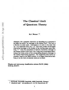
FIG. 1. Left: The contour Cv and deformed contour Cu∞ for the integral in (27) in the case when Γu and Γv have one connected component. Right: The contour Cu for the integral in (30). When Gv → Gu , the two logarithmic branch points on the first sheet join the two simple branch points at the extremities of Γu .
By the functional relations (14), similar representation holds for f large. For the complete solution we try an ansatz of the form I � dz ± iq± (z) � F (e ) , (18) Au± [f ] = exp 2π Cu
where the functions F ± can be expanded as ±
F (ω) =
F1± ω
+
F2± ω 2
+
F3± ω 3
+ ...,
(19)
with = ±1. The coefficients Fn can be determined by comparing with the exactly solvable case f (z) = κ, or q± (z) = −i log κ ± Gu (z), where [4] (20)
To compare with (18), we perform the contour integration using the asymptotics eiq± (z) ' (1 ± κ Nz ) at z → ∞, and find Fn± = ±1/n2 . Therefore F ± (z) = ±
∞ X zn = ± Li2 (z). n2 n=1
(21)
The functional equation for the dilogarithm, Li2 (1/z) = −Li2 (z) − π 2 /6 −
1 2
log2 (−z),
(22)
is the scaling limit of (14). 4. Classical limit of the Slavnov and Gaudin-Izergin determinants and of the Gaudin norm We will use the factorization formula (8) to find for the classical limit of the Slavnov determinant (5). In this limit we can consider U and V as c-number functions, since the they commute up to O(N −2 ). Then we can use the functional relation (14) to write (8) in the form Su,v = Av+ [κ eiGu −iGθ ] ] Au− [eiGv ] .
The integration contours Cu and Cv encircle Γu and Γv anticlockwise. The r.h.s. of (24) can be reformulated entirely in terms of the function q(z) defined in (25). The Bethe equations (2) imply a boundary condition for the resolvent Gu , 2/Gu (z) − Gθ (z) + log κ = 2πnk for z ∈ Γku , (26) where /Gu is the half-sum of the values of the resolvent on both sides of Γu and nk is the mode number associated with the k-th connected component Γku ⊂ Γu . Hence, if q (1) is the value of the function q(z) on the physical sheet defined by (25), then the value of q(z) on the second sheet is given by q (2) = −Gu + Gv and (24) can be written as I dz Li2 (ei q(z) ). (27) log Su,v = 2π Cu ∪Cv
F1±
Au± [κ] = (1 − κ)N .
(25)
(23)
Introduce, as in (15), the resolvents Gu , Gv and Gz , associated respectively with the sets of points u, v and z.
(The minus sign is compensated by the change of the orientation of contour Cu after it is moved to the first sheet.) The integral along Cu is however ambiguous, because the integrand has two logarithmic cuts which start at two branch points on the first sheet and end at z = ∞ on the second sheet, after crossing the cut of the resolvent Gu on Γu . The ambiguity is resolved by deforming the contour Cu to a contour Cu∞ which encircles also the point z = ∞ on the second sheet [10]. In the case of a one-cut solution, the contour Cu∞ is depicted in Fig. 1, left. With this prescription, eq. (24) reproduces the numerical data (for κ = −1 and N up to 60) with precision 10−12 . Another test of (27) is to send all the roots u to infinity. In this limit the integration goes only along the contour Cv and the function q in the integrand is given by q = Gv − 21 Gθ . Then eq. (27) reproduces correctly the expression obtained in [4] for the scalar product of Bethe state and a vacuum descendent. We will also need the classical limit of the GaudinIzergin determinant, for which (12) gives I � dz log Zu,v = − Li2 eiGv −iGu . (28) 2π Cu
Finally, an expression for the square of the Gaudin norm can be formally obtained from (27) by taking Gu = Gv = G. When Γv → Γu , the integration contour in (27) can be closed around Γu = Γv as in Fig. 1, right, and q in the integrand is replaced by 2pu , where pu = Gu − 21 Gθ +
1 2
log k
(29)
4 is the quasi momentum. Thus we find for the square of the Gaudin norm I � � dz (30) log Su,u = Li2 e2ipu (z) . 2π Cu
One can check, using the fact that p(z) = ±iπρ(z) on the two edges of the cut, that the contour integral (30) can be transformed into (twice) the linear integral in eq. (2.15) of [4].
nally obtain, up to a complex constant, I X � � dz 0 1 log C123 Li2 e2ipn (z) ' − 2 2π n=u,v,w Cn I � � dz + Li2 eipu (z)+ipv (z)+iL3 /2z 2π ∞ ∪C Cu v
I +
i h dz Li2 eipw (z)+i(L2 −L1 )/2z . 2π
(33)
Cw
V.
CLASSICAL LIMIT OF THE STRUCTURE CONSTANT
Now we can proceed with the computation of the classical limit of the structure constant (1), which we express in terms of the functionals considered above, 0 C123 =
Su,v∪z Zz,w . 1/2 1/2 1/2 Su,u Sv,v Sw,w
(31)
In applying (27), (28) and (30) the only non-obvious point is the evaluation of Su,v∪z with z = θ (13) + 2i . This is the the ‘restricted Slavnov product’ studied in [6, 11, 12], in which part of the magnon rapidities are frozen to the values of the impurities on a segment of the spin chain. In the original formulation (5), the restricted Slavnov product is given by a ratio of vanishing quantities, which necessitates to apply repeatedly l’Hˆopital’s rule. In contrast, the factorized representation (8) is free of such complications. It is given by the r.h.s. of (27), with (for κ = 1) q = Gu + Gv∪z − Gθ(12) ∪θ(13) = Gu + Gv − Gθ(12) .
(32)
Expressing the resolvents Gu , Gv , Gw in terms of the (1) (2) three quasi-momenta pu = Gu − 12 Gθ , pv = Gv − 21 Gθ (3) and pw = Gw − 12 Gθ , and taking the homogeneous limit θ (n) → 0, replacing Gθ(n) → Ln /2z (n = 1, 2, 3). we fi-
[1] J. A. Minahan and K. Zarembo, JHEP 03 (2003) 013, arXiv:hep-th/0212208. [2] N. Beisert et al, “Review of AdS/CFT Integrability: An Overview,” Lett. Math. Phys. 99 (Jan., 2012) 3–32, arXiv:hepth/1012.3982. [3] J. Escobedo, N. Gromov, A. Sever, and P. Vieira, arXiv:hep-th/1012.2475. [4] N. Gromov, A. Sever, and P. Vieira, arXiv:hep-th/1111.2349. [5] N. A. Slavnov, Russian Math. Surveys 62:4 (2007), 727. [6] O. Foda, arXiv:hep-th/1111.4663. [7] A. G. Izergin, Soviet Phys. Doklady 32 (Nov., 1987) 878. [8] V. E. Korepin, Comm. Math. Phys. 86 (1982) 391–418. [9] I. Kostov, to appear.
As it was pointed out by Gromov and Vieira in [13], 0 the tree level solution for C123 in presence of impurities (1) (2) (3) θ , θ , θ can be used to obtain the one-loop corrections. In this sense we have obtained also the correlator of three non-BPS classical fields at one-loop. The method outlined in this note allows to handle the impurities in the classical limit and attack the problem in its full generality. The expression (33) can be used [14] to show that, at least in the classical limit, the two-loop result is obtained by changing the quasimomenta pu , pv and pw according to the three-loop Bethe ansatz equations [15]. It is natural to expect that the full structure coefficient in the SU (2) sector in SYM will be obtained from (33) by using the exact expression for the quasimomenta upon inclusion of the dressing phase [16]. At least this possibility is worth of being explored and we hope to be able to report on this in a future publication.
ACKNOWLEDGMENTS
The author is obliged to S. Alexandrov, O. Foda, N. Gromov, A. Sever, D. Serban, P. Vieira and K. Zarembo for illuminating discussions, to P. Vieira and N. Gromov for conducting the numerical tests, and to P. Vieira and O. Foda for critical reading of the manuscript. Part of this work has been done during the visit of the author at Nordita in February 2012.
[10] The author is indebted to Nikolay Gromov for performing the numerical test and for suggesting how to place the integration contours. [11] N. Kitanine, J. M. Maillet, and V. Terras, Nucl. Phys. B 554 (1999) 647, arXiv:math-ph/9807020 [12] M. Wheeler, Nucl. Phys. B 852 (2011)468, arXiv:math-ph/1104.2113. [13] N. Gromov and P. Vieira, arXiv:hep-th/1202.4103. [14] D. Serban, arXiv:hep-th/1203.5842 [15] N. Beisert, V. Dippel, and M. Staudacher, JHEP 07 (2004) 075, arXiv:hep-th/0405001. [16] N. Beisert, B. Eden, and M. Staudacher, J. Stat. Mech. 0701 (2007) P021, arXiv:hep-th/0610251.