CLASSIFICATION OF BROADLEAF AND GRASS WEEDS USING GABOR WAVELETS AND AN ARTIFICIAL NEURAL NETWORK L. Tang, L. Tian, B. L. Steward ABSTRACT. A texture–based weed classification method was developed. The method consisted of a low–level Gabor wavelets–based feature extraction algorithm and a high–level neural network–based pattern recognition algorithm. This classification method was specifically developed to explore the feasibility of classifying weed images into broadleaf and grass categories for spatially selective weed control. In this research, three species of broadleaf weeds (common cocklebur, velvetleaf, and ivyleaf morning glory) and two grasses (giant foxtail and crabgrass) that are common in Illinois were studied. After processing 40 sample images with 20 samples from each class, the results showed that the method was capable of classifying all the samples correctly with high computational efficiency, demonstrating its potential for practical implementation under real–time constraints. Keywords. Broadleaf, Gabor wavelets, Grass, Neural network, Real–time, Selective weed control, Texture.
I
n post–emergence applications, broadleaf and grass weed classes are typically controlled differently with different selective herbicides or different tank mixes with corresponding application rates (Novartis, 1998). Therefore, if the spatial distribution of categories of broadleaf and grass weeds could be locally sensed, then selective herbicides could be applied on an intermittent or patch–spraying basis (Woebbecke et al., 1995a). Classification of weeds into broadleaf and grass categories is a less complex task for a real–time sensing system than individual species classification (Mortensen et al., 1998) and is consistent with current herbicide treatments (Johnson et al., 1995). This methodology represents an advancement over patch–spraying, which is only based on the presence or absence of weeds in a local area, and thus could potentially lead to more effective spatially selective weed control. Shape–based classification and texture–based classification are two approaches to weed species identification. Shape feature–based weed species classification has been conducted by numerous researchers (Guyer et al., 1986, 1993; Franz et al., 1991; Woebbecke et al., 1995b; Yonekawa et al., 1996). This approach, however, has limited application to plant canopies, as it demands analysis on the individual
Article was submitted for review in February 2002; approved for publication by Information & Electrical Technologies Division of ASAE in March 2003. Presented at the 1999 ASAE Annual Meeting as ASAE Paper No. 993036. The use of trade names is only meant to provide specific information to the reader and does not constitute endorsement of the product. The authors are Lie Tang, Assistant Professor, Agro Technology Group, Department of Agricultural Sciences, The Royal Veterinary and Agriculture University, Taastrup, Denmark; Lei F. Tian, ASAE Member Engineer, Associate Professor, Department of Agricultural Engineering, University of Illinois at Urbana–Champaign, Urbana, Illinois; and Brian L. Steward, ASAE Member Engineer, Assistant Professor, Agricultural and Biosystems Engineering Department, Iowa State University, Ames, Iowa. Corresponding author: Lei F. Tian, AESB 160, University of Illinois, 1304 W. Pennsylvania Ave., Urbana, IL 61801; phone: 217–333–7534; fax: 217–244–0323; e–mail: lei–
[email protected].
seedling or leaf level. Texture features derived from the color co–occurrence matrices have been applied in distinguishing plant and weed species. Shearer and Holmes (1990) used 33 color texture features derived from image intensity, saturation, and hue color attributes to classify seven common cultivars of nursery stocks and reported a 91% accuracy. Meyer et al. (1998) used four classical textural features for weed species discriminant analysis. Grass and broadleaf classification had a reported accuracy of 93% and 85%, respectively, while individual species classification accuracy ranged from 30% to 77%. The main limitation of the use of texture features for classification in real–time sensing applications is the large computation time required for feature extraction and classification, for example, 20 to 30 seconds on a UNIX workstation in the case of Meyer et al. (1998). In order for a real–time sensing system to be practical, it must be able to accurately classify weeds within real–time constraints. In more general texture research, Haralick et al. (1973) used co–occurrence matrices to classify different kinds of sandstone categories in photomicrograph images and land use in aerial and satellite images. Davis et al. (1979) indicated that using co–occurrence matrices for complex texture analysis is computationally intensive. Statistical methods, like using the co–occurrence spatial dependence method, have been shown to be superior to frequency domain techniques due to the lack of spatial locality in frequency domain methods (Weszka et al., 1976). Such methods as the Fourier transform can estimate spectral content of entire images but lose information about where in that image a spectral feature is located. Reed and Du Buf (1993) further concluded that joint space–frequency techniques are inherently local in nature, and are more computationally efficient than statistical methods. Joint space–frequency methods are able to measure the frequency content in localized regions in the spatial domain. These methods can overcome the drawbacks of traditional Fourier–based techniques, which can only provide global spatial frequency information. Extraction of local features
Transactions of the ASAE Vol. 46(4): 1247–1254
E 2003 American Society of Agricultural Engineers ISSN 0001–2351
1247
instead of global features enables the detection of continuity of a feature as well as the boundaries between different regions. Two excellent examples of local feature extractors are retinal and cortical cells in the human visual system. Experiments carried out by Porat and Zeevi (1989) on the human visual system have shown that both retinal and cortical cells can be characterized as having a limited extent of receptive field, and as such, can be described as local feature extractors. More specifically, cortical simple cells have been described as bar or edge detectors. As a mathematical counterpart, Gabor wavelets have been shown to resemble the receptive field profile of the simple cortex cells (Daugman, 1985). Bovik et al. (1990) demonstrated that 2–D Gabor filters are particularly useful for analyzing texture images containing highly specific frequency or orientation characteristics. Based on the research cited above, joint space–frequency texture features have potential for weed classification, but little research effort investigating this approach has been documented to date. An algorithm using these features could effectively classify weeds with varying canopy size and with high computational efficiency. Such an algorithm is needed to practically implement real–time weed sensing and classification into broadleaf and grass classes. These considerations provided the motivation for this research. OBJECTIVES The objectives of this research were to explore the feasibility of using Gabor wavelet–constructed spatial filters to extract texture–based features from field images and to use these extracted feature vectors to classify weeds into broadleaf and grass categories.
MATERIALS
The seeds of three broadleaf weed species Ĉ common cocklebur (Xanthium strumarium), velvetleaf (Abutilon theophrasti), and ivyleaf morning glory (Ipomoea hederacea) Ĉ and two grass species Ĉ giant foxtail (Setaria faberi) and crabgrass (Digitaria sanguinalis) Ĉ were manually planted at the University of Illinois Agricultural Engineering Research Farm on 28 May 1999. Each species was planted in a small plot, which measured 1.2 × 3.6 m (4 × 12 ft). Images were taken on 30 June 1999, approximately four weeks after seeding. The weeds were at a growth stage commonly seen when post–emergence herbicides are applied. A ViCAM video conferencing digital camera (Vista Imaging Inc., San Carlos, Cal.) connected to the USB port of a Compaq Presario laptop 1655 computer with a 266 MHz Pentium II processor was used to acquire a set of images. The camera was mounted on a tripod at a height of 1.4 m (55 in). The camera had a resolution of 640 × 480 pixels and used a standard ViCAM lens that had a 6.5 mm focal length and an F2.0 relative aperture. The lens had a 44° horizontal viewing angle and a 32° vertical viewing angle, which resulted in a field of view of 1.1 × 0.8 m (44 × 32 in.). Thus, the imaging system’s spatial resolution was approximately 1.7 × 1.7 mm (0.07 × 0.07 in.) per pixel in the 640 × 480 pixel images. The camera was manually white balanced through a calibration procedure using images of a white surface. The auto gain control was set at the peak mode, and the image quality control was set at the high–quality setting with 24–bit RGB
1248
color. The lighting illuminance and color temperature levels were recorded using a chroma meter (Model XY–1, Minolta, Ramsey, N.J.). During the entire image collection period, the illuminance and color temperature levels varied from 14,000 lux to 90,000 lux and from 5,800 K to 7,150 K, respectively. The shutter speed varied from 1/240 s to 1/3500 s, corresponding to the minimum and maximum intensity level. A set of ten velvetleaf, four ivyleaf morning glory, six common cocklebur, ten giant foxtail, and ten crabgrass images were acquired. The camera used a conventional CCD sensor, but its lens created blurring at the four image corners. Therefore, 300 × 250 pixel sub–images were cropped from the center of images and used in subsequent analysis. The feature extraction algorithm was written using Visual C++ 6.0 (Microsoft Corp., Redmond, Wash.). The artificial neural network (ANN) classifier was developed using the neutral network toolbox and Matlab script language in Matlab 4.0 (The MathWorks, Inc., Natick, Mass.).
METHODS
The Gabor wavelet/ANN system was developed to classify images of weeds into broadleaf and grass categories using texture features. There were two layers in this scheme. A Gabor wavelet–based algorithm extracted spatial–frequency texture features of the weed images, and a feedforward ANN processed the extracted feature vectors to classify the weed images. IMAGE PRE–PROCESSING Compared with general texture analysis applications, texture–based weed classification has particular characteristics. In this particular application, the texture pattern of interest was the characteristics of the frequency of reflectance changes across weed leaf areas. Background features should be minimized when extracting spatial frequency features from weed canopies. Meyer et al. (1998) indicated that weeds in field images must be carefully segmented; otherwise, the textural analysis will yield unreliable results by mixing soil and residue features with those from weeds. Weeds in the images were thus first segmented from the image background. Segmented images were used to constrain sampling to ensure that sampling points, which were the central locations of later convolution filtering used to extract features, were from known vegetation regions. Woebbecke et al. (1995a) examined several color indices for weed image segmentation and found that the excess green (ExG) and modified hue color indices yielded the best near–binary images of weeds. Meyer et al. (1998) also applied ExG to separate plant and soil regions for weed species identification research. The color index used for segmentation in this research was called modified excess green (MExG) and was defined as: MExG = 2 × G – R – B
(1)
where R, G, and B are the unnormalized red, green, and blue channel pixel intensities, with constraints: if (G < R or G < B or G < 120), then ExG = 0. Image artifacts generated by the camera used in this research motivated the modification of the excess green color index. One image artifact was a tendency for color saturation
TRANSACTIONS OF THE ASAE
(a)
(b)
(c)
(d)
(e)
Figure 1. Example green channel images (left column) and their corresponding binary images produced by weed segmentation where MExG = 25 was used as the segmentation threshold (right column). From top to bottom, the images contain: (a) crabgrass, (b) giant foxtail, (c) ivyleaf morning glory, (d) common cocklebur, and (e) velvetleaf.
to rise at plant edges. Another image artifact was caused by the red and blue channel signals decreasing to very low values Ĉ less than that of the green channel in some background areas where the intensity level was changing rapidly. To overcome these color artifacts, the above constraints were added to the ExG equation.
Vol. 46(4): 1247–1254
The segmentation threshold was determined manually by examining the MExG histogram “valleys” and also adjusted by visually observing segmentation results using a user interactive display function from Image–Pro Plus 3.0 software (Median Cybernetics, Silver Spring, Md.). An MExG threshold of 25 was used to segment all images (fig. 1).
1249
FEATURE EXTRACTION USING GABOR WAVELETS Gabor wavelets have been shown to resemble the receptive field profile of simple visual cortex cells, which can perform joint space–frequency analysis (Porat and Zeevi, 1989; Bovik et al., 1990, 1992; Reed and Du Buf, 1993; Mallat, 1996; Naghdy et al., 1996). This resemblance provided motivation for the development of a Gabor wavelets feature extractor. Human vision model research has suggested the existence of an internal space–frequency representation that is capable of preserving both local and global information (Beck et al., 1987). With the Fourier transform, it is not possible to do joint space–frequency analysis. In contrast, the short time Fourier transform (STFT) can achieve this function and is defined as: STFT(τ ω) = ∫ s(t )g(t − τ)exp(−j ωt )dt
(2)
From this definition, the STFT can be interpreted as the Fourier transform of a signal s(t) that is windowed by the function g(t – t). The STFT with a Gaussian window is called a Gabor transform. The Gabor transform can be regarded as a signal being convoluted with a filter bank, whose impulse response in the time domain is Gaussian modulated by sine and cosine waves. As the frequency (w) of the sine and cosine function changes, a set of filters with the same window size is constructed. A limitation of the STFT or Gabor transform is that the size of the window in the time/space domain is fixed, which results in a fixed resolution in both spatial and frequency domains. Therefore, the STFT and Gabor transform are suitable for analysis of stationary signals, which is not the case for most natural textures. This problem can be overcome by the wavelet transform that possesses resolution flexibilities in both spatial and frequency domains. In this research, the two dimensional (x and y) elementary Gabor wavelet function was used for weed feature extraction (Naghdy et al., 1996) and was defined as: x2 + y2 h(x, y) = exp− α2 j ⋅exp[j πα j(x cosθ + y sinθ)] 2
(3)
1 , j = 0,1,2..., and θ∈[0,2π0 . 2 The Gabor wavelet function is a two–dimensional Gaussian envelope with standard deviation a–j modulated by a sinusoid with frequency aj/2 and orientation q. The different choices of frequency level j and orientation q were used to construct a set of filters. As the frequency of the sinusoid changes, the window size changes. For example, when j is increased, the sinusoid frequency is reduced, whereas the Gaussian window size is increased. Similar to the STFT, wavelets can be viewed as band–pass filters and be implemented with a filter bank. This filter bank was composed of spatial domains filters that were generated from the elementary Gabor wavelet function. At each frequency level in the filter bank, there was a pair of filters that corresponded to the real and imaginary parts of the complex sinusoid in the Gabor wavelet function. The filter output at each frequency level was computed as: where α=
V[ j] = R 2j −ave + I2j −ave
(4)
where Rj–ave is the mean output of the real filter mask, and Ij–ave is the mean output of the imaginary filter mask, both at
1250
frequency level j across multiple sample points. At every frequency level, the filter bank produced one texture feature. Because multiple frequencies were used, the filter bank produced a multidimensional texture feature vector (V) for each instance it was applied. To apply the filter bank, each filter pair was convolved with a region of interest (ROI) at a sample point in a green channel image consisting of only segmented plants. The green channel image was chosen for feature extraction because this channel had better contrast between plants and soil than the other color channels. This higher contrast enabled the extraction of more salient texture features. FILTER FREQUENCY AND CONVOLUTION MASK SIZE SELECTION The filter bank was defined by the number and level of frequencies and the filter dimension or mask size. The filter orientation was fixed at 90° in this work. The choice of these parameters affected the efficacy as well as the computation efficiency of the classification system. Eight sample images containing all five weed species were randomly selected for an experiment to select these filter bank parameters. Ten frequency levels from 0 to 9 and three mask sizes of 9 × 9 pixels, 13 × 13 pixels, and 17 × 17 pixels were investigated to measure the effect of frequency level and mask size on class separability. Feature vectors were clearly affected by the frequency level and mask size (fig. 2). To reduce the computational burden, the filter banks should be made small, as long as adequate information needed to distinguish between classes can be provided to the high–level classifier. By analyzing the separation between classes of each feature, a filter bank with four frequency levels from 4 to 7 was determined to be suitable for the classification task. Mask size also affects the amount of computation needed to extract the features as well as classification accuracy. Generally, a larger mask size will be able to pick up more details in the texture image, but to meet real–time application constraints, the mask size should also be restricted. The separability of broadleaf and grass classes appeared to be substantially improved when the mask size was increased from 9 × 9 pixels to 13 × 13 pixels. Some additional improvement was observed when the mask size was further increased to 17 × 17 pixels (fig. 2). In this research, a mask size of 17 × 17 pixels was thus selected (fig. 3). SAMPLING POINT SELECTION Sample points in each image were selected randomly with the constraint that each point be segmented as a plant pixel, that is, its MExG value must be greater than the threshold of 25. In addition, the sample point had to be four–connected to other plant pixels in order to be considered as a valid plant pixel. By incorporating these selection constraints, the influence from “salt and pepper” noise in the images was substantially reduced. These randomly sampled points were the center points of the ROIs that were convolved with the Gabor wavelets filter masks. To extract texture features from an image, the filter bank was applied to many sample points, and the mean filter outputs were used to calculate the value of each feature. The number of sample points to be used for feature extraction was determined experimentally. Features were generated at 100, 150, and 200 random sample points in a set of sample images from both classes. For each sample point
TRANSACTIONS OF THE ASAE
Random sampling is important because it lowers the sensitivity of the feature extraction algorithm to sample point selection bias. Although the weed density or the vegetation area inside the images can vary significantly, the sample size (number of sampled vegetation pixels) need not necessarily be proportional to the population size (the total number of vegetation pixels available in an image). As stated by Stuart (1984), it is the sample size, and not the fraction of population sampled, that almost entirely determines the precision of estimation once the variability of population is given. These considerations, balanced with the increased computational burden with the increased number of sample points, led to the selection of 150 sample points for texture feature extraction (fig. 4).
filtering output
0.25
(a)
0.2 0.15 0.1 0.05 0
0
1
2
3
4
5
6
7
8
9
frequency level
filtering output
0.3
(b)
0.25 0.2 0.15 0.1 0.05 0
0
1
2
3
4
5
6
7
8
9
frequency level
filtering output
0.3
(c)
0.25 0.2 0.15 0.1 0.05 0
0
1
2
3
4
5
6
7
8
9
frequency level Figure 2. Feature vectors with ten frequency levels and mask sizes of: (a) 9 × 9, (b) 13 × 13, (c) 17 × 17. Solid and dashed lines represent broadleaf and grass–type weeds, respectively.
level, there were two or three repetitions of the sampling and feature extraction process. For every image, and for each sample point level, the mean variation among the features vectors from all repetitions was checked. Substantial variation was often observed between the feature vectors when the number of random sampling points was 100. When 150 and 200 random points were used, minor variation was observed for every tested image.
ANN CLASSIFICATION A three–layer feedforward backpropagation ANN was developed, trained, and used for classification. The choice of a backpropagation ANN as the high–level classifier was based on the fact that ANNs are computing systems whose central theme is borrowed from the analogy of biological neural networks. The main advantage of ANNs is that they can process information in parallel. Multilayer networks trained by the backpropagation algorithm are also capable of learning nonlinear decision surfaces. Even though the backpropagation algorithm can be trapped by local minima in the error surface, it is one of the most widely used ANN algorithms and has been found to produce excellent results in many real–world applications. With three layers of units, feedforward networks can approximate any function to arbitrary accuracy (Mitchell, 1997, pp. 191–196). The ANN classifier had a four–node input layer corresponding to the four–dimensional feature vector. The hidden layer consisted of eight nodes, while the output layer had two nodes, which corresponded to broadleaf and grass classes. The logarithmic sigmoid function was chosen as the threshold unit for all three layers, and the learning rate was set to one. Since the backpropagation algorithm is susceptible to overfitting the training examples at the cost of decreasing generalization accuracy over other unseen examples, several stopping criteria were investigated. A sum square error of 0.01 was selected as the stopping criterion for training, as it was observed to produce good classification results. The ANN was trained with a training set of 20 images, with 10 images from each class that were randomly selected from the set of 40 weed images. The training images were first processed with the Gabor wavelet feature extractor, and
Figure 3. Filter bank used in this research. From left to right are the filter masks from frequency levels 4 to 7. Top and bottom rows are real and imaginary filter masks, respectively. Filter mask size is 17 × 17 pixels.
Vol. 46(4): 1247–1254
1251
Image Pre–processing RGB color image of size 300 × 250 pixels Modified excess green image MExG = 2G–R–B
Green channel image splitting
Feature Extraction Generate 150 random points p(x,y), where MExG pixel value is greater than 25. Generate Gabor wavelets filter masks of size 17 × 17 with frequency level j from 4 to 7 at orientation of 90° At every frequency level j , convolve wavelets masks at each p(x,y) in green channel image and calculate the average of real(Rj–ave ) and imaginary (Ij–ave ) output from masks Save normalized modulation of convolution output from each filter as one feature. Output = sqrt(R2 j–ave + I 2j–ave ) Figure 4. Block diagram of image pre–processing and feature extraction algorithm.
the feature vectors were saved to a file before neural network training. The remaining 20 images were used as validation images and similarly processed by the feature extractor. The feature vectors were applied to the ANN, and the values of the output node were recorded.
RESULTS
The ANN training process converged quickly within 500 epochs. After training the ANN, application of the feature vectors from the broadleaf weed validation images to the input nodes of the ANN resulted in values from 0.989 to 0.995 at the broadleaf class output and from 0.003 to 0.015 at the grass class output. When the feature vectors from the grass weed validation images were applied, the broadleaf class output varied from 0.006 to 0.043 while at the grass node, the result varied from 0.958 to 0.996 (table 1). The value of an output node provides a measure of confidence ranging from 0 to 1 that an image belongs to a class, with 1
as the highest confidence. The results show that across this particular set of validation images, the classifier provided consistent results across the image in each class, with little sensitivity to particular species of weeds. In addition, all of the images could be correctly classified easily by a simple comparison of the output node values. The feature extraction algorithm was computationally efficient. For example, consider the case of an image of consisting of 300 × 250 pixels. With four frequency levels, there will be eight filter masks from both real and imaginary parts. With 150 random sample points and a mask size of 17 × 17 pixels, the number of multiplication and addition operations will be 346,800 (17 × 17 × 8 × 150). Comparing this computation load with simple one–run low–pass or high–pass filtering with a 3 × 3 pixel filter mask, the number of computations will be 298 × 248 × 3 × 3 (edge–trimmed image size × filter size). This filter operation thus requires 665,136 multiplications, which is about double the computation required for the feature extraction scheme. The computational time for feature extraction per image including all image pre–processing steps was measured. The average time was approximately 550 ms measured on a Pentium II 233 MHz computer. To evaluate the effectiveness of the classification method and the stability of the image sensor under natural outdoor lighting conditions, no artificial lighting or diffuser was used during image acquisition. The automatic functions provided by the camera driver were found to be useful in coping with outdoor lighting conditions. The auto gain control was especially effective in dealing with lighting intensity changes that often occur during the day. The image quality of the set of images used in this research was stable over a daylong image collection period.
SUGGESTIONS FOR FUTURE WORK
The results from the texture–based classification algorithm demonstrate the potential of this biologically inspired classifier for a real–time weed sensing system that has the capability to distinguish between broadleaf and grass weeds. In the current system, while the results are very good, there are several limitations, and correspondingly, several potential areas for future research. First, the feature extraction algorithm only applied unidirectional wavelet filters. This implies that the algorithm requires a difference in the width of broadleaf and grass leaves along a single direction. Although it is typically the case that broadleaf leaves are wider than grass leaves, it is not always true. The main difference between broadleaf leaves and grass leaves is that broadleaf leaves have rounded or
Table 1. ANN output node values resulting from the input of each validation feature vector. Output node values observed for each broadleaf weed validation image (output node classes B1 to B10) Broadleaf Grass
B1 0.993 0.004
Broadleaf Grass
G1 0.010 0.992
B2 0.993 0.015
B3 0.993 0.003
B4 0.993 0.007
B5 0.993 0.004
B6 0.993 0.003
B7 0.993 0.003
B8 0.995 0.003
B9 0.995 0.004
B10 0.989 0.007
Output node values observed for each grass weed validation image (output node classes G1 to G10)
1252
G2 0.008 0.992
G3 0.007 0.995
G4 0.007 0.995
G5 0.006 0.995
G6 0.037 0.961
G7 0.031 0.959
G8 0.006 0.996
G9 0.006 0.996
G10 0.043 0.958
TRANSACTIONS OF THE ASAE
slightly elliptic shapes, whereas grass leaves have elongated shapes. An asymmetric filter mask or multiple orientation filter masks with different mask size and frequency combinations could possibly pick up local spatial frequency changes, which are more pertinent to the natural difference between these two weed classes. In addition, with the adoption of a more diverse filter bank, the algorithm may be better able to cope with growth stage variations. Second, each weed image in this work contained only one weed species. Several common class species in a particular image may affect the broadleaf and grass classification task, and should be investigated. In the case of multiple class species co–existing in an image, which can happen frequently under field conditions, a method of texture–based segmentation, instead of just classification, needs to be developed. Texture–based segmentation represents a next step of this weed classification research. Another possible adaptation of this classification algorithm is to find the minimum broadleaf or grass cluster size from which the current classification algorithm can still extract separable features. This area could then be used as a scanning unit, and the image could thus be segmented into broadleaf areas, grass areas, or mixture areas at the resolution of this scanning unit based on the output value of the ANN classifier. Third, a fixed image resolution level was used in this research. For practical agricultural applications, it is important to consider ways to lower the cost of sensing equipment. Although the camera had a field of view corresponding to one and a half 0.76 m spaced crop rows, a larger field of view would lower the number of sensors required. Therefore, classification evaluation at different fields of view could reveal how large an area one sensor could cover. Finally, although the algorithm has shown promise for real–time implementation, the computational efficiency can be further improved. A major proportion of the computation burden came from the calculation of the MExG index for segmentation. Computation time could be saved from this process by using a look–up table, which trades computer memory for speed (Tian and Slaughter, 1998; Steward and Tian, 1998).
CONCLUSIONS
A pattern recognition system composed of a Gabor wavelet feature extractor and a feedforward backpropagation ANN classifier was developed to classify weeds into broadleaf and grass classes. Particularly, a Gabor wavelet filter bank was designed to obtain joint space–frequency characteristics from weed texture images. High classification accuracy obtained from a set of validation images demonstrated the potential of the method. When compared with other statistical methods of using co–occurrence matrices, the developed feature extraction algorithm is computationally efficient and thus presents advantages in meeting real– time requirements. ACKNOWLEDGEMENTS This material is based on work supported by the Illinois Council for Food and Agricultural Research under Award No. C–Far 1–5–95281 and University of Illinois. Any opinions, findings, and conclusions or recommendations expressed in this publication are those of the authors and do not
Vol. 46(4): 1247–1254
necessarily reflect the views of the Royal Veterinary and Agricultural University or the University of Illinois.
REFERENCES
Beck, J., A. Sutter, and R. Ivry. 1987. Spatial frequency channels and perceptual grouping in texture segregation. Computer Vision, Graphics, and Image Processing 37(2): 299–325. Bovik, A. C., M. Clark, and W. Geisler. 1990. Multichannel texture analysis using localized spatial filters. IEEE Trans. Pattern Analysis and Machine Intelligence 12(1): 55–73. Bovik, A. C., N. Gopal, T. Emmoth, and A. Restrepo. 1992. Localized measurement of emergent image frequencies by Gabor wavelets. IEEE Trans. Information Theory 38(2): 691–712. Daugman, J. G. 1985. Uncertainty relation for resolution in space, spatial frequency, and orientation optimized by two–dimensional visual cortical filters. J. Optical Society of America A 2(7): 1160–1169. Davis, L. S., S. A. Johns, and J. K. Aggarwal. 1979. Texture analysis using generalized co–occurrence matrices. IEEE Trans. Pattern Analysis and Machine Intelligence 1(2): 252–259. Franz, E., M. R. Gebhardt, and K. B. Unklesbay. 1991. The use of local spectral properties of leaves as an aid for identifying weed seedlings in digital images. Trans. ASAE 32(2): 682–687. Guyer, D. E., G. E. Miles, M. M. Shreiber, O. R. Mitchell, and V. C. Vanderbilt. 1986. Machine vision and image processing for plant identification. Trans. ASAE 29(6): 1500–1507. Guyer, D. E., G. E. Miles, L. D. Gaulttney, and M. M. Schreiber. 1993. Application of machine vision to shape analysis in leaf and plant identification. Trans. ASAE 36(1): 163–171. Haralick, R. M., K. Shanmugam, and I. Dinstein. 1973. Textural features for images classification. IEEE Trans. Systems, Man, and Cybernetics 3(2): 610–621. Johnson, G. A., D. A. Mortensen, and A. R. Martin. 1995. A simulation of herbicide use based on weed spatial distribution. Weed Research 35(1): 197–205. Mallat, S. 1996. Wavelets for a vision. Proc. IEEE 84(4): 604–614. Meyer, G. E., T. Mehta, M. F. Kocher, D. A. Mortensen, and A. Samal. 1998. Textural imaging and discriminant analysis for distinguishing weeds for spot spraying. Trans. ASAE 41(4): 1189–1197. Mitchell, T. M. 1997. Machine Learning. Boston, Mass.: WCB/McGraw–Hill. Mortensen, D. A., J. A. Dieleman, and G. A. Johnson. 1998. Weed spatial variation and weed management. In Integrated Weed and Soil Management, 293–309. J. L. Hatfield, D. D. Buhler, and B. A. Stewart, eds. Chelsea, Mich.: Ann Arbor Press. Naghdy, G., J. Wang, and P. Ogunbona. 1996. Texture analysis using Gabor wavelets. IS&T/SPIE Symp. Electronic Imaging. Proc. SPIE 2657: 74–85. Novartis. 1998. Sample Labels and Reference Guide. Greensboro, N.C.: Novartis. Porat, M., and Y. Y. Zeevi. 1989. Localized texture processing in vision: Analysis and synthesis in the Gaborian space. IEEE Trans. Biomedical Eng. 36(1): 115–129. Reed, T. R., and J. M. H. Du Buf. 1993. A review of recent texture segmentation and feature extraction techniques. Computer Vision Graphics and Image Processing: Image Understanding 57(3): 359–372. Shearer, S. A., and R. G. Holmes. 1990. Plant identification using color co–occurrence matrices. Trans. ASAE 33(6): 2037–2044. Stuart, A. 1984. The Ideas of Sampling. New York, N.Y.: Macmillan. Steward, B. L., and L. F. Tian. 1998. Real–time weed detection in outdoor field conditions. In Proc. SPIE 3543: Precision Agriculture and Biological Quality, 266–278. G. E. Meyer and J. A. DeShazer, eds. Bellingham, Wash: SPIE.
1253
Tian, L. F., and D. C. Slaughter. 1998. Environmentally adaptive segmentation algorithm for outdoor image segmentation. Computers and Electronics in Agric. 21(3): 153–168. Weszka, J. S., C. R. Dyer, and A. Rosenfeld. 1976. A comparative study of texture measures for terrain classification. IEEE Trans. Systems, Man, and Cybernetics 6(1): 269–285. Woebbecke, D. M., G. E. Meyer, K. Von Bargen, and D. A. Mortensen. 1995a. Color indices for weed identification under various soil, residue, and lighting conditions. Trans. ASAE 38(1): 259–269.
1254
Woebbecke, D. M., G. E. Meyer, K. Von Bargen, and D. A. Mortensen. 1995b. Shape features for identifying young weeds using image analysis. Trans. ASAE 38(1): 271–281. Yonekawa, S., N. Sakai, and O. Kitani, 1996. Identification of idealized leaf types using simple dimensionless shape factors by image analysis. Trans. ASAE 39(4): 1525–1533.
TRANSACTIONS OF THE ASAE