J. N. Am. Benthol. Soc., 2009, 28(4):869–884 ’ 2009 by The North American Benthological Society DOI: 10.1899/08-142.1 Published online: 29 September 2009
Classifying the biological condition of small streams: an example using benthic macroinvertebrates Kelly O. Maloney1
AND
Donald E. Weller2
Smithsonian Environmental Research Center (SERC), 647 Contees Wharf Rd., P.O. Box 28, Edgewater, Maryland 21037-0028 USA
Marc J. Russell3 Gulf Ecology Division, US Environmental Protection Agency, 1 Sabine Island Dr., Gulf Breeze, Florida 32561 USA
Torsten Hothorn4 Institut fu¨r Statistik, Ludwig-Maximilians-Universita¨t, Ludwigstraße 33, D-80539 Mu¨nchen, Germany
Abstract. The ability to classify the biological condition of unsurveyed streams accurately would be an asset to the conservation and management of streams. We compared the ability of 5 modeling methods (classification and regression trees, conditional inference trees, random forests [RF], conditional random forests [cRF], and ordinal logistic regression) to predict stream biological condition (very poor, poor, fair, or good) based on benthic macroinvertebrate Index of Biotic Integrity data taken from the Maryland Biological Stream Survey. Predictor variables included land use and land cover (e.g., impervious surface, row-crop agriculture, and population density) and landscape measures (annual precipitation and watershed area). We included 1561 sites on small nontidal streams in the Maryland portion of the Chesapeake Bay watershed. We used 1248 sites (80%) as a training data set to build models and 313 sites (20%) as an independent evaluation data set. RF and cRF models most accurately predicted observed integrity scores in the evaluation data set, but we selected the cRF as the best model because of weaknesses in the RF model (e.g., biased variable selection). Percent impervious surface was the most important variable in the cRF model, and the probability that a site was in very poor or poor biological condition increased rapidly as % impervious cover increased up to 20%. When applied to predict stream biological conditions in all 7908 small nontidal stream reaches in the study area, the cRF model predicted that 33.8% were in fair, 29.9% in good, 22.7% in poor, and 13.6% in very poor biological condition. Our analyses can be used to manage and conserve freshwater and estuarine resources of Maryland and the Chesapeake Bay watershed. Model predictions for unsurveyed streams can help target field studies to identify high-quality streams deserving of conservation and impaired streams in need of restoration. Key words: stream condition, landscape-scale, land use, random forests, conditional inference, classification and regression trees (CART), ordinal logistic regression, prediction.
Biological assessments have shown that many small streams have been impaired by anthropogenic stressors (Benke 1990, USEPA 2000). These results have generated much interest in conserving and managing these streams and their watersheds. However, small 1 2 3 4
streams are numerous (Leopold et al. 1964), and assessing the biological condition of all small streams is logistically impractical and cost prohibitive. Models that reliably predict biological conditions at unsurveyed locations are needed. One way to estimate regional biological conditions in streams and rivers is to extrapolate the observed proportions of impairment classifications from a sample of streams to all streams in a landscape (e.g., if 30% of the sampled sites are impaired, then 30% of the sites in the region are impaired; USEPA 2006). However, such results
E-mail addresses:
[email protected] [email protected] [email protected] [email protected]
869
870
K. O. MALONEY
provide limited information to managers who need estimates of biological condition for individual streams to target management efforts. Models that predict stream biological condition from watershed attributes, such as watershed size, human population, and land use/land cover, could provide reach-specific biological condition estimates for unsurveyed locations and could help quantify how watershed attributes affect stream biological condition. Classification and regression trees (Breiman 1984, De’ath and Fabricius 2000, Loh 2008) are statistical techniques that might be useful for constructing classification models for predicting stream biological condition. Such models are being applied more often in ecology, partly because they can handle complex data sets with higher-order interactions and nonlinear relationships (Breiman 1984, De’ath and Fabricius 2000). Robust models are useful for stream classification and prediction because the relationships between stream biological conditions and stressors are complex. For example, land cover often is used as a surrogate for anthropogenic stressors in watersheds and streams. However, percentages of land cover in different categories often are correlated with each other or with natural gradients, and land cover data can have interactive and nonlinear relationships with stream biological condition (Allan 2004, King et al. 2005, Walton et al. 2007). Tree models explain variation in categorical (classification trees) or continuous (regression trees) response variables as a function of §1 explanatory variables, which also can be categorical or continuous. Many algorithms exist for constructing classification or regression trees (e.g., C4.5, CART, CRUISE, GUIDE, and QUEST; Loh 2008), but most follow a simple general scheme. A covariate is selected from all available exploratory variables, and a split point that separates the response values into 2 homogenous groups is estimated. For a continuous explanatory variable, such as precipitation, the split point is determined by a numerical value of the explanatory variable. For a categorical variable, such as ecoregion, the 2 groups are defined by the set of levels of the explanatory variable to which the observations belong. Once the split point has been estimated for a selected explanatory variable and the groups have been defined, each group is further separated with new explanatory variables and split points. A predefined stopping criterion is used to end the recursive splitting procedure. Recent advances in the field of machine learning have increased the accuracy and the predictive ability of single-tree models by using ensembles of trees (forests; Cutler et al. 2007). This approach averages the predictions of multiple trees (e.g., 500) generated from
ET AL.
[Volume 28
a permutated subsample of the data set. Random forests (RF) are one of the simplest examples of such a procedure (Breiman 2001, Liaw and Wiener 2002, Cutler et al. 2007). In RF, bootstrap samples are drawn with replacement from the original data set. Observations not included in a bootstrap sample are named out-of-bag observations. A very large tree is generated for each bootstrap sample, and is used to classify the out-of-bag observations; i.e., the tree predicts (votes for) the class of the out-of-bag observations. The overall predicted class for each sample in the original data set is the classification that receives the most votes. RF-type models do not provide an easily interpretable relationship between the response variable and the predictor variables (unlike CART or linear regression). However, inferences about the relationships between predictor and response variables can be drawn from variable importance plots and partial dependence plots. Variable importance is calculated for each predictor variable by randomly permuting the values of the variable for the out-of-bag observations. These modified out-of-bag observations are passed through the tree to obtain new predictions. The importance of the variable is the difference between the misclassification rate for the modified and original out-of-bag observations divided by the standard error (Cutler et al. 2007). CART and ensemble tree methods show promise for developing predictive-based models for stream biological condition, but their efficacy has not been evaluated or compared for streams. We compared results from 5 models that classified biological condition of small nontidal streams in the Maryland portion of the Chesapeake Bay watershed. We built models with Brieman’s CART algorithm and its ensemble-tree analog (RF). However, CART and RF models are biased because they select against categorical explanatory variables and treat ordinal response variables as nominal (Hothorn et al. 2006, Strobl et al. 2007, Loh 2008). This bias could lead to incorrect inferences between responses and predictors. Therefore, we also built models with conditional inferences trees (cTREE) and an ensemble-tree method based on these trees (conditional random forests [cRF]). cTree methods use classical statistical tests (Hothorn et al. 2006) to select a split point based on the minimum p-value among all tests of independence between the response variable and each explanatory variable. cTREEs and cRFs derive unbiased estimates of explanatory variables and correctly handle ordinal response variables (Hothorn et al. 2006, Strobl et al 2007). We also built a model using ordinal logistic regression (OLR) because OLR has been successfully used to classify ecological condition (Bigler et al. 2005).
2009]
CLASSIFYING STREAM INTEGRITY
871
FIG. 1. The Maryland portion of the Chesapeake Bay watershed, its major ecoregions (Omernik 1987), and stream assessment points with data for benthic macroinvertebrates. Inset shows the study area (dark gray) in relation to the Chesapeake Bay watershed (light gray) and 7 states in the mid-Atlantic region of the USA. DE = Delaware, MD = Maryland, NJ = New Jersey, NY = New York, PA = Pennsylvania, VA = Virginia, WV = West Virginia.
We built models with a training data set in which stream biological condition (assessed with a benthic macroinvertebrate Index of Biotic Integrity [IBI]) was the dependent variable, and watershed attributes, including measures of natural landscape variation (e.g., watershed area and elevation), climate (precipitation), and anthropogenic stressors represented by land cover (e.g., % impervious cover, % row-crop cover) were explanatory variables. We evaluated models with an independent validation data set. We applied the best of the models to predict stream biological conditions in all small nontidal streams in the Maryland portion of the Chesapeake Bay watershed. Methods Study area Maryland is in the Mid-Atlantic region of the US (Fig. 1) and encompasses an area of 31,873 km2. We focused on the 23,408-km2 part of Maryland in the Chesapeake Bay watershed (Fig. 1), which includes 6 Level III ecoregions: Central Appalachians, Ridge and Valley, Blue Ridge, Northern Piedmont, Southeastern Plains, and Middle Atlantic Coastal Plains (Omernik
1987). Climate types range from cold with hot summers in the mountainous western area to temperate with hot summers toward the southeast (Peel et al. 2007). Vegetation patterns range from northern hardwood forests in the highlands to oak, hickory, pine, and southern mixed forests of the Coastal Plains (Omernik 1987). The Appalachian, Ridge and Valley, and Blue Ridge ecoregions are underlain mainly by folded and faulted sedimentary rocks; the Piedmont ecoregion is underlain by crystalline igneous and metamorphic rocks; and the Plains ecoregions are underlain by unconsolidated sediments (Edwards 1981). Stream types range from coldwater streams in the highland ecoregions (Central Appalachians and Ridge and Valley) to blackwater streams of the Coastal Plains (MDDNR 2005). Macroinvertebrate indices of biotic integrity We obtained benthic macroinvertebrate data from the Maryland Biological Stream Survey (MBSS; USEPA 1999). MBSS scientists used a probabilistic sampling design stratified by major watershed and stream order (1st- to 4th-order streams as shown on
872
K. O. MALONEY
ET AL.
[Volume 28
TABLE 1. Summary statistics for explanatory watershed variables used in models. * indicates variables highly correlated with other variables and, therefore, eliminated from model development (see Methods). Count = number of sites in each ecoregion. Abbreviation PerPast PerCrop PerExtr PerTree PerImp Pop* Elevation* Slope* Precip WSArea Latitude Longitude Ecoregion
Description % of watershed under pasture cover % of watershed under row-crop cover % of watershed under extractive (i.e., mining) cover % of watershed under tree cover % of watershed under impervious cover Human population density (no. persons/km2) Average watershed elevation (m) Average slope of watershed (%) Average watershed annual precipitation (cm) Watershed area (km2) Latitude in decimal degrees Longitude in decimal degrees Dominant Omernik (1987) Level III ecoregion of watershed
1:100,000 US Geological Survey [USGS] maps; Southerland et al. 2005b) to sample ,2500 streams from 1994 to 2004. We used the benthic macroinvertebrate IBI data from these samples in our models (Southerland et al. 2005b). We used data from streams with watershed areas ,200 km2 and that were in the Chesapeake Bay watershed. We used only the first record for sites that were sampled more than once. Of the ,2500 samples, 1561 satisfied these conditions. In the MBSS survey, benthic macroinvertebrates were sampled with a D-frame net from all habitats within a 75-m stream reach (Klauda et al. 1998), and subsampled to 100 organisms. Insects were identified to genus level (Southerland et al. 2005b). Watershed characteristics We modeled the relationships between the recorded IBI at each sampling point and the attributes of the watershed draining to the sampling point (Table 1). We used watershed boundaries delineated in previous studies (King et al. 2005) with methods described in Baker et al. (2006). We summarized watershed attributes by overlaying watershed boundaries on spatial data sets for land cover, human population, and elevation. We calculated percentages of each land cover in the entire watershed of each sampling point and within a 100-m riparian buffer of the upslope stream network for each site. Riparian conditions are good predictors of stream biological condition (e.g., Strayer et al. 2003, King et al. 2005). We estimated the percentage of each area (watershed or 100-m riparian
Range/ecoregion
Mean
0–84.0 0–85.6 0–24.7 0.7–99.0 0–61.3 0–7598 0.8–876.7 0.0–17.2 93.8–126.8 0.1–197.1 38.02–39.72 279.40 to 275.32 Blue Ridge Central Appalachians Mid-Atlantic Coastal Plain Northern Piedmont Ridge and Valley Southeastern Plains
16.3 15.5 0.2 35.9 5.3 303 170.3 4.2 112.3 20.5 39.22 276.97
Count
58 44 191 542 134 279
buffer) covered by impervious surface, trees, rowcrop agriculture, pasture, and extractive cover (e.g., mines) from land cover, tree cover, and impervious surface maps derived from circa 2000 Landsat images (RESAC 2000) with methods later adopted by federal agencies for the National Land Cover Database (Huang et al. 2001, Yang et al. 2003, Homer et. al. 2004). Population block data also were overlaid with watershed boundaries, and population density was calculated as the no. people/km2 (US Census 2000). For partial census blocks within a watershed, we estimated the population contributing to the watershed total by multiplying the percentage of the census block within the watershed by the total population within the census block (i.e., we assumed a homogenous population distribution within the census block). We calculated average watershed slope and elevation from a digital elevation model (DEM) and average annual precipitation for each watershed from a publicly available data set (PRISM Climate Group 2006) using Zonal Statistics (++) in Hawth’s Analysis Tools for ArcGIS (Beyer 2007). During preliminary variable screening, we found that all riparian land cover proportions except extractive land cover (r = 0.39) were highly correlated with whole watershed proportions (all r . 0.65), slope and elevation were highly correlated with longitude (both r . 0.80), and population density was highly correlated with impervious surface (r = 0.78). Therefore, % land covers in the 100-m riparian buffer, slope, elevation, and population density were eliminated from further model development.
2009]
CLASSIFYING STREAM INTEGRITY
Model development We used a random subsample of 80% of the sites selected from the MBSS database as a training data set for model development (n = 1248), and we reserved the remaining 20% for an independent data set for model validation (n = 313). The same training and validation data sets were used for every model. All analyses were done with R statistical software (R Development Core Team 2008). We built models to relate the benthic IBI classification of stream biological condition (very poor, poor, fair, or good) to the explanatory variables describing watersheds. Our 1st model was a classification tree model using CART (Brieman 1984; R package rpart; http:// cran.r-project.org/web/packages/rpart/index.html). Many user-defined stopping criteria options can be chosen for the traditional CART model (e.g., no samples misclassified, end nodes reach a threshold homogeneity, or a set minimum number of samples/ node is attained; McCune and Grace 2002). We set the minimum number of samples to create a split at 10, the minimum number of observations in a terminal node (or leaf) at 7, the complexity parameter (cp; a threshold at which any split that does not decrease the lack of fit by the value of cp is not done) at 0.001, and the number of cross-validation procedures at 20. We used the 1-SE rule, which does an internal 10-fold cross validation to select the largest cp with a cross-validation error ƒ1 standard deviation (SD) of the minimum to prune our models (see Venables and Ripley 1999). Our 2nd model was an ensemble-tree analog (RF) based on CART (R package randomForest; http://cran.r-project.org/ web/packages/randomForest/index.html). We built 500 trees using default values for other parameters in the randomForest package. Our 3rd model was a cTREE (R package party, cTREE function; http:// cran.r-project.org/web/packages/party/index.html). We set the p-value to define a split at 0.05 (the analysis stops when no split is found below this criterion). We used default values for all other parameters. Our 4th model was an ensemble-tree analog (cRF) based on cTREE (R package party, cforest function). We used the default parameters for forest construction. For single-tree methods (CART, cTREE), we present the relationships between the response variable and explanatory variables with a dichotomous tree diagram with nodes that represent split points, branches that connect nodes, and leaves or terminal nodes that represent the final groups. For the ensemble-tree methods (RF, cRF), we present partial dependence plots constructed by plotting observed values of a certain predictor variable against the predicted status of the response variable on a probability scale to
873
illustrate the regression relationship between the response and explanatory variables. Our 5th model was fit with OLR. OLR selects an optimal combination of the explanatory variables for predicting an ordinal response variable, much like multiple linear regression analysis does for a continuous response variable. However, unlike linear regression, which models changes in the response variable, OLR models changes in the log odds (the natural logarithm of the odds ratio) of the response variable. OLR yields easily interpreted models and does not assume normality or homogeneity of variance in the response variable. OLR does require that explanatory variables be linearly related to the logit of the response variable. We fit a proportional odds model to the data (R Design Package, lrm function; http://cran.r-project.org/web/packages/ Design/index.html) and reduced model complexity by backwards elimination using the Akaike Information Criterion (AIC) for variable removal until the lowest AIC was achieved. Preliminary diagnostics indicated possible nonlinear relationships between the biological condition category and % pasture cover, so we also tested a 2nd-order polynomial for this explanatory variable during model construction. Model accuracy We evaluated model performance with 3 commonly used accuracy measures: percentage of observations correctly classified (PCC), weighted k, and the area under the receiver operating characteristic curve (AUC). Each of these measures has specific advantages and disadvantages (Harrell 2001, McPherson et al. 2004), and models are best assessed with several accuracy measures (e.g., Fielding and Bell 2002, Cutler et al. 2007, Rutherford et al. 2007). Both PCC and weighted k are derived from the model confusion matrix, a table that contrasts predicted vs observed classifications. Weighted k adjusts PCC for agreement caused by chance alone and gives more importance to more similar classes (Cohen 1968, Meyer et al. 2008, Fleiss and Cohen 1973). Values of weighted k range from 21 to 1. Positive values indicate that the classification is more successful than would be expected from chance alone, whereas negative values indicate worse results than expected from chance alone. A value of +1 indicates perfect agreement between the modeled and measured classifications (Cohen 1960). AUC evaluates the sensitivity (true positives) and specificity (false positives) of the model. AUC values range from 0 to 1, with values .0.5 indicating model performance better than would be expected from chance alone and a value of +1
874
K. O. MALONEY
indicating perfect agreement (Swets 1988). We calculated AUC values with the ordROC function in the nonbinROC R package (http://cran.r-project.org/ web/packages/nonbinROC/index.html). We used a weighted penalty matrix in which sites incorrectly classified by 3 categories (e.g., a very poor site misclassified as good) were weighted 33 as much as sites incorrectly classified by 1 category (e.g., a fair site misclassified as good). Sites incorrectly classified by 2 categories were weighted 23 as much as sites incorrectly classified by 1 category. For every model, we calculated each accuracy measure in 2 ways. First, we calculated each accuracy measure for the confusion matrix from the training data set (resubstitution method; Cutler et al. 2007). Second, we calculated each accuracy measure for the confusion matrix from the validation data set. We put greater emphasis on the validation results because we were most interested in the ability of models to predict stream biological conditions at unsurveyed sites. Prediction of stream biological condition in the Maryland portion of the Chesapeake Bay watershed We predicted stream biological condition (very poor, poor, fair, good) for all (7908) small (,200 km2 watershed area) nontidal streams in the Maryland portion of the Chesapeake Bay watershed. We applied the best of the models to stream reaches and associated watersheds in the 1:100K National Hydrography Dataset plus (NHDplus; USGS 2006). The NHDplus data set is based on the same 1:100,000 USGS maps as were used to select sites for the stream surveys. We calculated attributes for each NHDplus watershed with methods detailed above using the entire watershed draining to the downstream end of a reach. Results The CART model produced a pruned tree with 14 splits and 15 terminal nodes (Fig. 2), and the cTREE model produced a tree with 10 splits and 11 terminal nodes (Fig. 3). Both models split sites based on % impervious cover (PerImp; CART PerImp = 6.6%, cTREE PerImp = 6.5%). Both models split sites with PerImp greater than these levels into terminal nodes for sites in fair and very poor biological condition based on % wetland cover (PerWet). However, sites with lower PerImp levels were modeled differently by the CART and cTREE models. The CART model split this subset by longitude, whereas the cTREE model split it again by PerImp. The CART model had several terminal nodes for sites in poor or good biological condition, whereas the cTREE model had 1 terminal node for sites in each of these biological conditions (Figs 2, 3).
ET AL.
[Volume 28
In the RF and cRF models, PerImp was the most important variable, and precipitation (Precip) and % tree cover (PerTree) were among the 4 most important variables for both models (Fig. 4A, B). In the RF model, longitude was the 2nd most important variable, and ecoregion was the 3rd least important variable. However, in the cRF model, ecoregion was the 4th most important variable, and longitude the 5th most important. These results might indicate a bias against selecting categorical variables in the RF model. Partial dependence plots show the relationship between a particular predictor variable and the response variable. As an example, we present these plots for PerImp for both the RF and cRF models (Figs 5A–D, 6A–D). As PerImp increased from 0 to 20%, both models showed a rapid increase in the probability that a site would be classified as in very poor or poor biological condition (Figs 5A, B, 6A, B) and a rapid decrease in the probability that a site would be classified as in fair biological condition (Figs 5C, 6C). The probability that a site would be classified as in good biological condition decreased sharply over a smaller increase in PerImp (0–15%) in both models (Figs 5D, 6D). When Precip ,,110 cm, RF and cRF models indicated a high probability that a site would be classified as in very poor or poor biological condition, and a low probability of being classified as in good biological condition. At values .110 cm, the probability that a site would be classified as in good biological condition was high and the probabilities that a site would be classified as in very poor and poor biological condition were low (data not shown). As PerTree increased, RF and cRF models showed decreasing probability that a site would be classified as in very poor or poor biological condition and increasing probability that a site would be classified as in good biological condition. The probability that a site would be classified as in fair biological condition increased as PerTree rose from 0 to ,25% and then decreased as PerTree rose further to ,80% (data not shown). In the RF model, more westward sites (lower longitude) had higher probabilities of being classified as in very poor or poor biological condition and lower probabilities of being classified as in fair or good biological condition (data not shown). In the cRF model, sites in the Southeastern Plains ecoregion had the highest probabilities of being classified as in fair or good biological condition and lowest probabilities of being classified as in very poor or poor biological condition. Sites in the Blue Ridge ecoregion had the highest probabilities of being classified as in very poor or poor biological condition and the lowest probabilities of being classified as in fair or good biological condition (data not shown).
2009]
CLASSIFYING STREAM INTEGRITY
875
FIG. 2. Classification tree from the Classification and Regression Tree (CART) model based on the training data set. Values on lines connecting explanatory variables indicate splitting criteria (e.g., if a site had ,6.6% PerImp then it was placed in the group to the right on the branch, otherwise it was placed on the branch to the left). Numbers in boxes above the explanatory variable indicate the node number. Numbers in parentheses next to terminal nodes indicate the number of sites classified in that node. The overall predicted biological condition for each terminal node is in italics in the boxes. Bar graphs illustrate the proportion of sites in measured biological condition in that node. V = very poor, P = poor, F = fair, G = good. See Table 1 for variable names.
The best OLR models (those with the lowest AICs) were 7- and 6-variable models (Appendix 1). Both models included linear relationships with PerTree, PerImp, Precip, % row-crop cover (PerCrop), and ecoregion, and a nonlinear relationship with % pasture cover (PerPast). The 7-variable model also included a linear relationship with PerWet (Appendix 1). The 2 models were comparable according to AIC (DAIC = 0.95, evidence ratio = 1.61), and both models explained the same amount of variation in IBI (both R2 = 0.28), so we selected the simpler 6-variable model as the best OLR model. For OLR, variable importance (VI) can be calculated by subtracting a variable’s degrees of freedom from its Wald x2 (Harrell 2001). For the 6-variable model, ecoregion was the most important variable (x2 = 107.7, df = 5, VI = 102.7, followed by PerTree (x2 = 46.7, df = 1, VI = 45.7), PerCrop (x2 = 28.3, df = 1, VI = 27.3), PerImp
(x2 = 25.5, df = 1, VI = 24.5), Precip (x2 = 22.1, df = 1, VI = 21.1), PerPast (x2 = 9.7, df = 2, VI = 7.7), and PerWet (x2 = 3.0, df = 1, VI = 2.0). In this model, the log odds of stream biological condition decreased significantly (p , 0.05) with the amounts of PerImp and PerWet in a watershed, but increased with PerTree, Precip, and PerCrop. Model accuracy Both CART and cTREE models classified ,½ of the validation sites correctly (PCC , 50%; Table 2), and weighted k values indicated that CART and cTREE model predictions of biological condition were slightly better than predictions based on chance alone (0.57 and 0.58, respectively). AUC indicated that both models performed better than chance alone (0.61, 0.61, respectively; Table 2). RF and cRF models also
876
K. O. MALONEY
ET AL.
[Volume 28
FIG. 3. Classification tree from the conditional inference tree (cTree) model. See Fig. 2 for an explanation of the organization of the tree. BR = Blue Ridge, CA = Central Appalachians, CP = Mid-Atlantic Coastal Plains, NP = Northern Piedmont, RV = Ridge and Valley, SP = Southeastern Plains.
classified ,½ of the validation sites correctly (Table 2), but weighted k values and AUC indicated that RF and cRF models performed equally well and better than CART and cTREE models (Table 2). The OLR performed worst according to PCC and weighted k values, but AUC suggested the OLR model predicted as well as CART and cTREE models. CART and cTREE models had high misclassification error rates for validation sites that were in poor biological condition (0.91 and 0.97, respectively), but both models had low misclassification rates for validation sites that were in very poor biological condition (both error rates = 0.25; Table 3). Validation sites in good biological condition were most often misclassified as being in fair biological condition, and sites in fair biological condition were most often misclassified as being in good biological condition by both single-tree models. RF and cRF models had high misclassification error rates for validation sites that were in poor biological condition (error rate = 0.63 and
0.79, respectively), and sites in this category were misclassified as being in good, fair, and very poor biological condition. Validation sites in good biological condition were misclassified most often as being in fair biological condition, and sites in fair biological condition were misclassified most often as being in good biological condition by both ensemble-tree models. Like the other models, the OLR model misclassified sites in poor biological condition most often (error rate = 0.77). Sites in good biological condition were misclassified most often being in fair biological condition, sites in fair biological condition were misclassified most often as being in good biological condition, and sites in very poor biological condition were misclassified most often as being in poor biological condition (Table 3). Across all models, sites in good biological condition rarely were misclassified as being in poor or very poor biological condition, and sites in very poor biological condition rarely were misclassified as being in good biological condition.
2009]
CLASSIFYING STREAM INTEGRITY
877
FIG. 5. Partial dependence plots for % impervious surface cover (PerImp) in the random forests (RF) model for classification of stream biological condition based on a benthic macroinvertebrate Index of Biotic Integrity for sites in very poor (A), poor (B), fair (C), and good (D) biological condition categories. Vertical hash marks on the x-axes indicate the deciles of the data distribution of the variable.
FIG. 4. Variable importance plots from the random forests (A) and conditional random forests (B) models for classification of stream biological condition based on a benthic macroinvertebrate Index of Biotic Integrity. Variables more important to the classifications have larger values for mean decrease of accuracy. See Table 1 for variable names.
biased against selecting categorical variables and treats ordinal variables as nominal variables. The cRF model predicted 29.9% of NHDplus streams to be in good biological condition, 33.8% to be in fair biological condition, 22.7% to be in poor biological condition, and 13.6% to be in very poor biological condition (Table 4). Sites that were predicted to be in poor biological condition were concentrated near urban areas (Fig. 7), and the distribution of predicted biological conditions differed among ecoregions (Fig. 7, Table 4). The most frequent predicted biological conditions were fair in the Blue Ridge, Central Appalachian, and Ridge and Valley ecoregions; poor in the Mid-Atlantic Coastal Plain; and good in the Southeastern Plains. Predicted biological conditions in the Northern Piedmont were more evenly distributed across the 4 categories. Discussion Model performance
Prediction of stream biological condition for the Maryland portion of the Chesapeake Bay watershed We used the cRF model to predict stream biological condition for all small nontidal stream reaches in the Maryland portion of the Chesapeake Bay watershed. The RF and cRF models performed equally well and better than CART, cTREE, or OLR (Table 2). We chose the cRF over the RF model because the RF algorithm is
We tested the ability of 5 modeling techniques to predict stream biological condition from watershed attributes. Two of these techniques, CART and cTREE, yield intuitive output that is easy to interpret. However, reliance on a single tree yields weak predictive ability, and these models can fail to predict some categories of nominal or ordinal data, as evidenced by their high misclassification error rates
878
K. O. MALONEY
ET AL.
[Volume 28
TABLE 2. Accuracy measures for predictions of biological condition for stream sampling sites in the Maryland portion of the Chesapeake Bay watershed. Resub = resubstitution accuracy estimates (model evaluated with same data used for calibration), Eval = accuracy estimates for an independent data set not used in calibration, PCC = % correctly classified, AUC = area under the receiver operating characteristic curve. Values in boldface indicate the weighted k and AUC accuracy statistic for the evaluation data set. Accuracy measure Classification method Classification trees
FIG. 6. Partial dependence plots for % impervious surface cover (PerImp) in the conditional random forests (cRF) model for classification of stream biological condition based on a benthic macroinvertebrate Index of Biotic Integrity for sites in very poor (A), poor (B), fair (C), and good (D) biological condition categories. Vertical hash marks on the x-axes indicate the deciles of the data distribution of the variable.
for sites in poor biological condition (Table 4). Multiple-tree analogs (RF and cRF) have fewer such weaknesses than do single-tree models. RF and cRF models performed similarly and predicted measured biological condition in a validation data set more accurately than did the single-tree methods or the OLR model (weighted k, AUC; Table 2). RF models are consistently better predictors than are CART models (Gislason et al. 2006, Cutler et al. 2007), but our study is the first to show that cRF models have better predictive ability than do cTree models in an ecological setting. In studies that generate categorical or ordinal data, the cRF model is more appropriate than the RF model because the RF model is biased against selecting categorical variables and treats ordinal data as nominal data (Strobl et al. 2007). Across all models and biological condition categories, most misclassifications occurred between adjacent biological condition categories. For example, 44 of the 47 sites in good biological condition were misclassified as being in fair biological condition by the cRF model, only 3 were misclassified as being in poor biological condition, and none were misclassified as being in very poor biological condition (Table 3). All models weakly discriminated between adjacent categories, and this weakness reduced overall model accuracies. However, all models accurately separated sites in very poor or poor biological
Conditional classification trees Random forests Conditional random forests Ordinal logistic regression
Estimate
PCC
Resub Eval Resub Eval Resub Eval Resub Eval Resub Eval
50.6 49.5 44.6 45.0 46.4 49.2 65.5 47.6 39.8 42.5
Weighted k AUC 0.58 0.57 0.54 0.58 0.55 0.62 0.75 0.64 0.48 0.55
0.65 0.61 0.58 0.61 0.64 0.69 0.80 0.68 0.58 0.62
condition from sites in good biological condition. Therefore, the models could be applied to distinguish high-quality streams deserving of conservation efforts from impaired streams in need of restoration. We tested how the accuracy of the cRF model would change if we used only 2 biological condition categories (good and very poor). Model accuracy improved significantly, and the cRF model correctly classified 40 of 48 (83%) sites in the validation data set as being in very poor biological condition and 94 of 103 (91%) sites as being in good biological condition. These rates of classification success are nearly double those of the model built using all 4 biological condition categories. However, considerable information is lost by removing the poor and fair categories because predictions for unsurveyed locations are limited to either very poor or good ratings. A better approach might be to use the probability of membership in a biological condition category provided by each model (see below). Important independent variables VI and partial dependence plots help identify the variables contributing most to stream impairment and quantify how those variables affect stream biological condition. PerImp was the most important variable influencing stream biological condition in our RF and cRF models (Fig. 4A, B) and in previous research (Paul and Meyer 2001, Wang and Lyons 2003, King et
2009]
CLASSIFYING STREAM INTEGRITY
879
TABLE 3. Confusion matrices for models for the training and evaluation data sets. Error rate is the fraction of sites that were misclassified. CART = classification and regression tree, cTree = conditional inference tree, RF = random forests, cRF = conditional random forests, OLR = ordinal logistic regression. Data set
Model CART
cTree
RF
cRF
OLR
Training
Validation
Biological condition class
Very poor
Poor
Fair
Good
Very poor
Poor
Fair
Good
Very poor Poor Fair Good Error rate Very poor Poor Fair Good Error rate Very Poor Poor Fair Good Error rate Very Poor Poor Fair Good Error rate Very Poor Poor Fair Good Error rate
150 16 49 20 0.36 143 3 77 12 0.39 125 63 26 21 0.47 157 47 23 8 0.33 89 74 54 18 0.62
97 41 112 68 0.87 89 10 200 19 0.97 68 87 114 49 0.73 54 143 90 31 0.55 50 98 117 53 0.69
26 11 221 108 0.40 24 2 287 53 0.22 20 82 164 100 0.55 7 41 251 67 0.31 16 84 154 112 0.58
7 9 93 220 0.33 5 0 207 117 0.64 9 27 90 203 0.38 2 7 54 266 0.19 2 35 136 156 0.53
36 2 5 5 0.25 36 0 12 0 0.25 26 14 7 1 0.46 31 9 6 2 0.35 23 17 8 0 0.52
18 6 29 17 0.91 18 2 44 6 0.97 13 26 18 13 0.63 15 15 30 10 0.79 12 16 26 16 0.77
8 3 54 27 0.41 7 1 69 15 0.25 5 17 40 30 0.57 4 11 47 30 0.49 2 17 48 25 0.48
3 1 40 59 0.43 3 0 66 34 0.67 0 7 34 62 0.40 0 3 44 56 0.46 1 8 48 46 0.55
al. 2005, Walsh et al. 2005). Impervious surface changes the patterns and magnitudes of stream flows, which in turn alter stream geomorphology (Booth and Jackson 1997, Paul and Meyer 2001, Wang and Lyons 2003). Impervious surface also increases the delivery of nutrients, metals, and other contaminants to streams (Paul and Meyer 2001), further degrading biological conditions. Stream habitat and communities change when the percentage of impervious surface in a watershed reaches 10 to 15% (Booth and Jackson 1997, Paul and Meyer 2001, Wang and Lyons 2003, King et al. 2005), and our models show a rapid increase in the probability that a site will be classified as in very poor or poor biological condition as PerImp rises from 0 to 20% (Figs 5A–D, 6A–D). Carlisle et al. (2009) recently used RF modeling to show a similar increase in the probability of changes in benthic assemblages as high-density residential development in a 100-m riparian zone increased from 0 to 10% cover. Such analyses are useful for developing conservation and land-management strategies because they document the relationships between land use and stream biological conditions.
The VIs of precipitation and ecoregion/longitude in the models probably were related, and demonstrate the need to account for physiographic variation when examining land-cover and ecological relationships (Poff et al. 2006). In our training data set, average watershed annual precipitation differed among ecoregions (ANOVA, F = 202, p , 0.001). Watersheds in the Blue Ridge and Central Appalachian ecoregions receive higher precipitation than watersheds in the Ridge and Valley and Southeastern Plains ecoregions (Tukey Honestly Significant Difference test, all p , 0.01). Such climate differences can influence the effect of land cover on instream biological conditions (Kaushal et al. 2008, Palmer et al. 2008). Ecoregion was unimportant in the RF model and very important in the cRF model, probably because the RF algorithm is biased against selecting categorical variables (Hothorn et al. 2006). The cRF model overcomes this bias and should provide sounder rankings of environmental factors for guiding conservation and management decisions. PerTree was one of the 4 most important variables in both the RF and cRF models (Fig. 4A, B), and the
880
K. O. MALONEY
ET AL.
[Volume 28
TABLE 4. Stream biological condition predicted by conditional random forests (cRF) model for all small nontidal watersheds in the Maryland portion of the Chesapeake Bay watershed. Numbers in parentheses are % of total sites in an ecoregion. cRF Ecoregion Blue Ridge Central Appalachians Mid-Atlantic Coastal Plain Northern Piedmont Ridge and Valley Southeastern Plains All
Very poor 5 21 3 684 115 248 1076
(2.7) (10.6) (0.1) (25.1) (13.7) (13.4) (13.6)
probability that a site was in fair or good biological condition increased with PerTree. Other studies also have reported that benthic biotic integrity, macroinvertebrate richness, and abundance measures of sensitive taxa all increase with forest cover in a watershed (Roth et al. 1996, Strayer et al. 2003). Higher tree cover also is correlated with smaller percentages of impervious surface, agricultural land, and other land covers that impose anthropogenic stressors on streams (King et al. 2005). Predicting stream biological condition for the Maryland portion of the Chesapeake Bay watershed We selected the cRF model to predict unsurveyed stream biological conditions for small nontidal
Poor 74 41 927 509 104 141 1796
(39.6) (20.6) (44.0) (18.7) (12.4) (7.6) (22.7)
Fair 108 89 694 718 478 585 2672
(57.8) (44.7) (32.9) (26.4) (56.8) (31.6) (33.8)
Good 0 48 484 811 144 877 2364
(0.0) (24.1) (23.0) (29.8) (17.1) (47.4) (29.9)
streams in the Maryland portion of the Chesapeake Bay watershed because other models (CART, cTREE, OLR) had weaker performance or known weaknesses (CART, RF). Others have applied RF and OLR models successfully to predict biological conditions in unsurveyed locations (Bigler et al. 2005, Carlisle et al. 2009), but we are unaware of any similar application of cRF models. The MBSS was a statewide probability-based survey with spatially intensive sampling, so the sample provides a good estimate of statewide stream integrity. MBSS estimates of the percentages of sites in the 4 biological condition categories were 26 6 1.3% (SE) in good, 28 6 1.5% in fair, 30 6 1.5% in poor, and 16 6 1.2% in very poor biological condition (Southerland et al. 2005a). The cRF model predictions for all
FIG. 7. Maps of predicted biological condition of small nontidal stream reaches in the Maryland portion of the Chesapeake Bay watershed. Biological condition was predicted from the conditional random forests model. Black polygons indicate areas of urbanization. Inset shows an enlarged view of the model output for the area around Frederick, Maryland.
2009]
CLASSIFYING STREAM INTEGRITY
stream reaches in our study area were 29.9% in good, 33.8% in fair, 22.7% in poor, and 13.6% in very poor biological condition. Model estimates for all categories were within 5% of the MBSS percentages, and the small differences probably were the result of our exclusion of sites with watershed area .200 km2 or outside the Chesapeake Bay watershed. Unlike the statewide extrapolation from sampled streams (Southerland et al. 2005a), our models also were able to provide a reach-specific prediction of biological condition for every small stream in the study area. Such predictions can be mapped to help guide research and management efforts (Fig. 7). We assigned each reach to the biological condition category with the highest probability, but all models provided probability of membership in each category. These probabilities are useful because they provide a measure of confidence in the predictions. For example, a model might assign site A probabilities of 0.20, 0.20, 0.29, and 0.31 for very poor, poor, fair, and good categories, respectively, and assign site B probabilities of 0.08, 0.02, 0.05, and 0.85. Although both sites are most likely to be in good biological condition, we can be more confident about the biological condition of site B than of site A. These probabilities can be used to prioritize costly conservation or restoration efforts by identifying sites where confidence about current biological condition is highest. Predicted stream biological conditions varied among ecoregions (Table 4), probably because of regional differences in percentages of land cover types. The high percentages of sites predicted to be in very poor and poor biological condition in the Northern Piedmont probably was the result of high average PerImp (5.1%) and low average PerTree (25.7%) in this ecoregion. The prevalence of sites predicted to be in poor biological condition in the Middle Atlantic Coastal Plains probably was related to low average PerTree (26.8%). The relatively high percentages of sites predicted to be in fair or good biological condition in the Southeastern Plains might have been related to low average PerCrop (6.0%) and PerPast (8.4%), even though this ecoregion had the highest average PerImp (7.2%). The Blue Ridge, Ridge and Valley, and Central Appalachian ecoregions all had relatively high percentages of sites predicted to be in fair biological condition, probably because these ecoregions had high average PerTree (62.1%, 63.1%, 72.7%, respectively) and PerPast (14.4%, 14.4%, 8.5%, respectively). Management implications Effective conservation and land management strategies require scientifically sound estimates of biological condition over large geographic areas, including at
881
sites where biological data are unavailable. Past research has identified the effects of anthropogenic disturbance on ecosystem structure and function and has provided the necessary scientific background for broad regional studies. Recent advances in computational power, spatial-analysis software (geographic information systems), statistical methods, and digital geographic data provide the data and tools needed to make generalizations and predictions over large areas. We combined these resources to construct models that predicted biological condition for all small nontidal stream reaches in the Maryland portion of the Chesapeake Bay watershed. The models were not useful for separating sites in intermediate biological condition categories (i.e., poor and fair) from sites in adjacent categories (very poor and good), but were useful for separating sites in good biological condition from sites in very poor biological condition. Therefore, the models can help conservation and land managers identify high-quality streams deserving of conservation and badly impaired streams in need of restoration. Acknowledgements Funding for our work was provided by the US Environmental Protection Agency National Center for Environmental Research (NCER) Science to Achieve Results (STAR) grant #R831369. Kevin Sigwart, Melissa Whitman, and Katie Sullivan helped with database synthesis and metric calculations. We thank Kathy Boomer, Lori Davias, Leska Fore, Pamela Silver, and 2 anonymous referees for comments that greatly improved the manuscript. We thank Andrew Liaw from Merck Research Laboratories for help with the RF algorithm, Frank Harrell, Jr. from Vanderbilt University for assistance with the Design package, and David Koons from Utah State University for assistance with the OLR analysis. We also thank the Maryland Department of Natural Resources for providing benthic macroinvertebrate data sets. The research described in this article has been funded by the US Environmental Protection Agency, but it has not been subjected to the Agency’s required peer and policy review and, therefore, does not necessarily reflect the views of the Agency and no official endorsement should be inferred. Literature Cited ALLAN, J. D. 2004. Landscapes and riverscapes: the influence of land use on stream ecosystems. Annual Review of Ecology, Evolution, and Systematics 35:257–284. BAKER, M. E., D. E. WELLER, AND T. E. JORDAN. 2006. Improved methods for quantifying potential nutrient interception by riparian buffers. Landscape Ecology 21:1327–1345.
882
K. O. MALONEY
BENKE, A. C. 1990. A perspective on America’s vanishing streams. Journal of the North American Benthological Society 9:77–98. BEYER, H. L. 2007. Hawth’s Analysis Tools for ArcGIS. (Available from: http://www.spatialecology.com/htools/) BIGLER, C., D. KULAKOWSKI, AND T. T. VEBLEN. 2005. Multiple disturbance interactions and drought influence fire severity in Rocky Mountain subalpine forests. Ecology 86:3018–3029. BOOTH, D. B., AND C. R. JACKSON. 1997. Urbanization of aquatic systems: degradation thresholds, stormwater detection, and the limits of mitigation. Journal of the American Water Resources Association 33:1077– 1090. BREIMAN, L. 1984. Classification and Regression Trees. Wadsworth International Group, Belmont, California. BREIMAN, L. 2001. Random forests. Machine Learning 45: 5–32. CARLISLE, D. M., J. FALCONE, AND M. R. MEADOR. 2009. Predicting the biological condition of streams: use of geospatial indicators of natural and anthropogenic characteristics of watersheds. Environmental Monitoring and Assessment 151:143–160. COHEN, J. 1960. A coefficient of agreement for nominal scales. Educational and Psychological Measurement 20: 37–46. COHEN, J. 1968. Weighted kappa: nominal scale agreement provision for scaled disagreement or partial credit. Psychological Bulletin 70:213–220. CUTLER, D. R., T. C. EDWARDS, K. H. BEARD, A. CUTLER, AND K. T. HESS. 2007. Random forests for classification in ecology. Ecology 88:2783–2792. DE’ATH, G., AND K. E. FABRICIUS. 2000. Classification and regression trees: a powerful yet simple technique for ecological data analysis. Ecology 81:3178–3192. EDWARDS, J. 1981. A brief description of the geology of Maryland. Maryland Geological Survey, Baltimore, Maryland. FIELDING, A. H., AND J. F. BELL. 2002. A review of methods for the assessment of prediction errors in conservation presence/absence models. Environmental Conservation 24:38–49. FLEISS, J. L., AND J. COHEN. 1973. The equivalence of weighted kappa and the intraclass correlation coefficient as measures of reliability. Educational and Psychological Measurement 33:613–619. GISLASON, P. O., J. A. BENEDIKTSSON, AND J. R. SVEINSSON. 2006. Random Forests for land cover classification. Pattern Recognition Letters 27:294–300. HARRELL, F. E. 2001. Regression modeling strategies with applications to linear models, logistic regression, and survival analysis. Springer Science+Business Media, Inc., New York. HOMER, C., C. Q. HUANG, L. M. YANG, B. WYLIE, AND M. COAN. 2004. Development of a 2001 National Land-Cover Database for the United States. Photogrammetric Engineering and Remote Sensing 70:829–840. HOTHORN, T., K. HORNIK, AND A. ZEILEIS. 2006. Unbiased recursive partitioning: a conditional inference frame-
ET AL.
[Volume 28
work. Journal of Computational and Graphical Statistics 15:651–674. HUANG, C., L. YANG, B. K. WYLIE, AND C. G. HOMER. 2001. A strategy for estimating tree canopy density using Landsat-7 ETM+ and high resolution images over large areas. Pages 230–240 in Proceedings of the 3rd International Conference on Geospatial Information in Agriculture and Forestry, 5–7 November 2001, Denver, Colorado. Veridian Environmental Research Institute of Michigan International, Inc., Ann Arbor, Michigan. KAUSHAL, S. S., P. M. GROFFMAN, L. E. BAND, C. A. SHIELDS, R. P. MORGAN, M. A. PALMER, K. T. BELT, C. M. SWAN, S. E. G. FINDLAY, AND G. T. FISHER. 2008. Interaction between urbanization and climate variability amplifies watershed nitrate export in Maryland. Environmental Science and Technology 42:5872–5878. KING, R. S., M. E. BAKER, D. F. WHIGHAM, D. E. WELLER, T. E. JORDAN, P. F. KAZYAK, AND M. K. HURD. 2005. Spatial considerations for linking watershed land cover to ecological indicators in streams. Ecological Applications 15:137–153. KLAUDA, R., P. KAZYAK, S. STRANKO, M. SOUTHERLAND, N. ROTH, AND J. CHAILLOU. 1998. Maryland Biological Stream Survey: a state agency program to assess the impact of anthropogenic stresses on stream habitat quality and biota. Environmental Monitoring and Assessment 51:299–316. LEOPOLD, L. B., M. G. WOLMAN, AND J. P. MILLER. 1964. Fluvial processes in geomorphology. W. H. Freeman, San Francisco, California. LIAW, A., AND W. WIENER. 2002. Classification and regression by randomForest. R News 2:18–22. LOH, W. Y. 2008. Classification and regression tree methods. Pages 315–323 in F. Ruggeri, R. S. Kenett, and F. W. Faltin (editors). Encyclopedia of statistics in quality and reliability. Wiley, Chichester, UK. MCCUNE, B., AND J. B. GRACE. 2002. Analysis of ecological communities. MjM Software Design, Gleneden Beach, Oregon. MCPHERSON, J. M., W. JETZ, AND D. J. ROGERS. 2004. The effects of species’ range sizes on the accuracy of distribution models: ecological phenomenon or statistical artefact? Journal of Applied Ecology 41:811–823. MDDNR (MARYLAND DEPARTMENT OF NATURAL RESOURCES). 2005. Maryland wildlife diversity conservation plan. Maryland Department of Natural Resources, Annapolis, Maryland. (Available from: http://dnr.maryland.gov/ wildlife/divplan_wdcp.asp) MEYER, D., A. ZEILEIS, AND K. HORNIK. 2008. Visualizing categorical data. Package vcd. R Foundation for Statistical Computing, Vienna, Austria. (Available from: http:// cran.r-project.org/web/packages/vcd/index.html) OMERNIK, J. M. 1987. Ecoregions of the conterminous United States. Annals of the Association of American Geographers 77:118–125. PALMER, M. A., C. A. REIDY LIERMANN, C. NILSSON, M. FLO¨RKE, J. ALCAMO, P. S. LAKE, AND N. BOND. 2008. Climate change and the world’s river basins: anticipating management options. Frontiers in Ecology and the Environment 6: 81–89.
2009]
CLASSIFYING STREAM INTEGRITY
PAUL, M. J., AND J. L. MEYER. 2001. Streams in the urban landscape. Annual Review of Ecology and Systematics 32:333–365. PEEL, M. C., B. L. FINLAYSON, AND T. A. MCMAHON. 2007. Updated world map of the Koppen-Geiger climate classification. Hydrology and Earth System Sciences 11: 1633–1644. POFF, N. L., B. P. BLEDSOE, AND C. O. CUHACIYAN. 2006. Hydrologic variation with land use across the contiguous United States: geomorphic and ecological consequences for stream ecosystems. Geomorphology 79: 264–285. PRISM CLIMATE GROUP. 2006. Parameter-elevation Regressions on Independent Slopes Model (PRISM). PRISM Climate Group, Oregon State University, Corvallis, Oregon. (Available from: http://www.prism.oregonstate.edu/) R DEVELOPMENT CORE TEAM. 2008. R: a language and environment for statistical computing. R Foundation for Statistical Computing, Vienna, Austria. RESAC (REGIONAL EARTH SCIENCE APPLICATIONS CENTER). 2000. 2000 land cover map of the Chesapeake Bay watershed. Mid-Atlantic Regional Earth Science Applications Center (RESAC), Department of Geology, University of Maryland, College Park, Maryland. (Available from: http://www.geog.umd.edu/resac/) ROTH, N. E., J. D. ALLAN, AND D. L. ERICKSON. 1996. Landscape influences on stream biotic integrity assessed at multiple spatial scales. Landscape Ecology 11:141–156. RUTHERFORD, G. N., A. GUISAN, AND N. E. ZIMMERMANN. 2007. Evaluating sampling strategies and logistic regression methods for modelling complex land cover changes. Journal of Applied Ecology 44:414–424. SOUTHERLAND, M. T., L. A. ERB, G. M. ROGERS, AND P. F. KAZYAK. 2005a. Maryland Biological Stream Survey 2000–2004, Volume VII: Statewide and tributary basin results. DNR-12-0305-0109. Chesapeake Bay and Watershed Programs, Maryland Department of Natural Resources, Annapolis, Maryland. SOUTHERLAND, M. T., G. M. ROGERS, M. J. KLINE, R. P. MORGAN, D. M. BOWARD, P. F. KAZYAK, R. J. KLAUDA, AND S. A. STRANKO. 2005b. Maryland Biological Stream Survey 2000–2004, Volume XVI: New biological indicators to better assess the condition of Maryland streams. DNR12-0305-0100. Maryland Department of Natural Resources, Annapolis, Maryland. STRAYER, D. L., R. E. BEIGHLEY, L. C. THOMPSON, S. BROOKS, C. NILSSON, G. PINAY, AND R. J. NAIMAN. 2003. Effects of land cover on stream ecosystems: roles of empirical models and scaling issues. Ecosystems 6:407–423. STROBL, C., A. L. BOULESTEIX, A. ZEILEIS, AND T. HOTHORN. 2007. Bias in random forest variable importance measures:
883
illustrations, sources and a solution. BMC Bioinformatics 8:25. doi:10.1186/1471-2105-8-25. SWETS, J. A. 1988. Measuring the accuracy of diagnostic systems. Science 240:1285–1293. US CENSUS. 2000. United States Census 2000. US Census Bureau, Department of Commerce, Washington, DC. (Available from: http://www.census.gov/main/www/ cen2000.html) USEPA (US ENVIRONMENTAL PROTECTION AGENCY). 1999. From the mountains to the sea: the state of Maryland’s freshwater streams. EPA/903/R-99/023. Office of Research and Development, US Environmental Protection Agency, Washington, DC. USEPA (US ENVIRONMENTAL PROTECTION AGENCY). 2000. 2000 National water quality inventory. Assessment and Watershed Protection Division (4503T), US Environmental Protection Agency, Washington, DC. USEPA (US ENVIRONMENTAL PROTECTION AGENCY). 2006. Wadeable Streams Assessment: a collaborative survey of the Nation’s streams. EPA 841-B-06-002. Office of Water, US Environmental Protection Agency, Washington, DC. USGS (US GEOLOGICAL SURVEY). 2006. National Hydrography Dataset (NHD) plus. Horizon Systems, Herndon, Virginia. (Available from: http://www.horizon-systems. com/nhdplus/) VENABLES, W. N., AND B. D. RIPLEY. 1999. Modern applied statistics with S-PLUS. 3rd edition. Springer-Verlag, New York. WALSH, C. J., A. H. ROY, J. W. FEMINELLA, P. D. COTTINGHAM, P. M. GROFFMAN, AND R. P. MORGAN. 2005. The urban stream syndrome: current knowledge and the search for a cure. Journal of the North American Benthological Society 24: 706–723. WALTON, B. M., M. SALLING, J. WYLES, AND J. WOLIN. 2007. Biological integrity in urban streams: toward resolving multiple dimensions of urbanization. Landscape and Urban Planning 79:110–123. WANG, L., AND J. LYONS. 2003. Fish and benthic macroinvertebrate assemblages as indicators of stream degradation in urbanizing watersheds. Pages 227–249 in T. P. Simon (editor). Biological response signatures: indicator patterns using aquatic communities. CRC Press, New York. YANG, L. M., G. XIAN, J. M. KLAVER, AND B. DEAL. 2003. Urban land-cover change detection through sub-pixel imperviousness mapping using remotely sensed data. Photogrammetric Engineering and Remote Sensing 69: 1003–1010. Received: 7 October 2008 Accepted: 18 August 2009
PerTree + PerImp + Precip + PerCrop + PerPast** + PerWet + Ecoregion PerTree + PerImp + Precip + PerCrop + PerPast** + Ecoregion Latitude + PerTree + PerImp + Precip + PerCrop + PerPast** + PerWet + Ecoregion WSArea + Latitude + PerTree + PerImp + Precip + PerCrop + PerPast** + PerWet + Ecoregion WSArea + Latitude + PerTree + PerImp + Precip + PerExtr + PerCrop + PerPast** + PerWet + Ecoregion WSArea + Longitude + Latitude + PerTree + PerImp + Precip + PerExtr + PerCrop + PerPast** + PerWet + Ecoregion PerTree + PerImp + Precip + PerCrop + PerWet + Ecoregion PerTree + PerImp + Precip + PerCrop + Ecoregion WSArea + PerTree + PerImp + Precip + PerCrop + PerWet + Ecoregion WSArea + Latitude + PerTree + PerImp + Precip + PerCrop + PerWet + Ecoregion WSArea + Latitude + PerTree + PerImp + Precip + PerCrop + PerPast + PerWet + Ecoregion WSArea + Latitude + PerTree + PerImp + Precip + PerExtr + PerCrop + PerPast + PerWet + Ecoregion WSArea + Longitude + Latitude + PerTree + PerImp + Precip + PerExtr + PerCrop + PerPast + PerWet + Ecoregion Null
Model 0.00 0.95 1.81 3.49 5.15 6.31 6.50 6.68 8.51 10.51 12.45 14.07 15.45 360.43
3078.3 3079.4 3079.6 3079.8 3081.6 3083.6 3085.6 3087.2 3088.6 3433.5
DAIC
3073.1 3074.0 3074.9 3076.6
AIC
13 2
0.00 2.20E279
0.00
0.02 0.02 0.01 0.01 0.00 0.00
0.03
0.41 0.25 0.16 0.07
Akaike weight
2269.92 1.85E+78
1135.69
23.46 25.82 28.26 70.53 191.52 506.49
13.14
1.00 1.61 2.47 5.72
Evidence ratio
0.27
0.27
0.28 0.27 0.27 0.27 0.27 0.27
0.28
0.28 0.28 0.28 0.28
R2
K. O. MALONEY
12
14 8 7 9 10 11
13
10 9 11 12
k
APPENDIX. Ordinal logistic regression (OLR) models ranked in order of increasing Akaike Information Criterion (AIC). k = number of variables used in AIC calculation. Variables with superscript ** were modeled with 2nd-order polynomials. Variable abbreviations are given in Table 1. The model in bold was selected as the best OLR model.
884 ET AL.
[Volume 28