Classifying Very High-Dimensional Data with Random Forests Built ...

44 International Journal of Data Warehousing and Mining, 8(2), 44-63, April-June 2012

Classifying Very High-Dimensional Data with Random Forests Built from Small Subspaces Baoxun Xu, Harbin Institute of Technology Shenzhen Graduate School, China Joshua Zhexue Huang, Shenzhen Institutes of Advanced Technology and Chinese Academy of Sciences, China Graham Williams, Shenzhen Institutes of Advanced Technology, and Chinese Academy of Sciences, China Qiang Wang, Harbin Institute of Technology Shenzhen Graduate School, China Yunming Ye, Harbin Institute of Technology Shenzhen Graduate School, China

ABSTRACT The selection of feature subspaces for growing decision trees is a key step in building random forest models. However, the common approach using randomly sampling a few features in the subspace is not suitable for high dimensional data consisting of thousands of features, because such data often contains many features which are uninformative to classification, and the random sampling often doesn’t include informative features in the selected subspaces. Consequently, classification performance of the random forest model is significantly affected. In this paper, the authors propose an improved random forest method which uses a novel feature weighting method for subspace selection and therefore enhances classification performance over high-dimensional data. A series of experiments on 9 real life high dimensional datasets demonstrated that using a subspace size of  log 2 (M ) + 1 features where M is the total number of features in the dataset, our random forest model significantly outperforms existing random forest models. Keywords:

Classification, Decision Tree, High-Dimensional Data, Random Forests, Random Subspace

1. INTRODUCTION One of the major current challenges to many classical classification algorithms is dealing

DOI: 10.4018/jdwm.2012040103

with large high dimensional data. Examples include text data, microarray data and digital images which often have thousands of features and hundreds of thousands or millions of objects. Such very high dimensional data has two special characteristics that affect the performance of classification algorithms. One is that different

Copyright © 2012, IGI Global. Copying or distributing in print or electronic forms without written permission of IGI Global is prohibited.

International Journal of Data Warehousing and Mining, 8(2), 44-63, April-June 2012 45

classes of objects are present in subspaces of the data dimensions. For example, in text data, documents relating to sport are categorized by the key words describing sport, while documents relating to music are represented by the key words describing music. The other characteristic is that a large number of dimensional features are uninformative to the class feature. That is, many features are only weakly correlated to the class feature, if at all and have a low power in predicting object classes (Saxena & Wang, 2010). The random forest (Breiman, 2001) algorithm is a popular classification method used to build ensemble models of decision trees from subspaces of data. Experimental results have shown that random forest models can achieve high accuracy in classifying high dimensional data (Banfield et al., 2007). Interest in random forests has grown in many domains where high dimensional data is prominent, including domains such as bioinformatics (Pang et al., 2006; Diaz-Uriarte & De Andres, 2006; Chen & Liu, 2005; Bureau et al., 2005), medical data mining (Ward et al., 2006) and image classification (Bosch, Zisserman, & Muoz, 2007). Several methods have been proposed to build random forest models from subspaces of data (Breiman, 2001; Ho, 1995, 1998; Dietterich, 2000). Among them, Breiman’s method (Breiman, 2001) has been popular due to its good performance compared to other methods (Banfield, Hall, Bowyer, & Kegelmeyer, 2007). Breiman uses a simple random sampling from all the available features to select subspaces when growing unpruned trees within the random forest model. Breiman suggested selecting  log 2 (M ) + 1 features in a subspace, where M is the total of independent features in data. This works well for data with certain dimensions (e.g., less than 100 features) but is not suitable for very high dimensional data consisting of thousands of features. In contrast, for very high dimensional data, Breiman’s subspace size of  log 2 (M ) + 1 is too small. Such data are dominated by uninformative features which have very low predictive power with respect to the target classification. Using a simple random

sampling results in informative features not being included in subspaces (Amaratunga, Cabrera, & Lee, 2008). As a result, weak trees are created and classification performance of the random forest is significantly affected. To increase the chance of selecting informative features in subspaces, the subspace size has to be enlarged extensively. However, this increases the computational requirements of the algorithm and increases the likelihood of the resulting trees being correlated. Correlated trees reduce the classification performance of a random forest model (Breiman, 2001). To address this problem Amaratunga (Amaratunga, Cabrera, & Lee, 2008) proposed a feature weighted method for subspace sampling. The weight of a feature is computed with respect to the correlation between the feature and the class. The weights are treated as the probability with which a feature is selected for inclusion in a subspace. Using this feature weighted method to sample subspaces there is a high chance that informative features are selected when growing trees for a random forest model. This method might be compared to the method of Adaboost (Freund & Schapire, 1996; Qiu, Wang, & Bi, 2008) which selects training samples according to the sample weights computed from the result of the previous classification. Such a method increases the probability for selecting informative features for inclusion in each subspace. This results in an increase in the average strength of the trees making up the random forest model, and thus the generalization error bound is reduced. Consequently, classification performance of the random forest model is increased. Amaratunga’s method is only valid for two-class problems, using the t-test of variance analysis to calculate the feature weights. In this paper, we propose a feature weighting method for subspace selection to solve multi-class problems. Instead of the t-test we calculate the chi-square statistic or information gain ratio as the feature weights. Both measures capture the correlation between a feature and the class for multi-class problems. The larger the weight, the more informative the feature to the classification. We normalize the set of weights to



sum to 1 and treat the normalized weights as the probability of selecting a feature within a subspace. We then use weighted sampling to randomly select feature subspaces with a high chance of including informative features. In this way, we increase the classification accuracy of the random forest model without the need to increase the subspace size from Breiman’s  log 2 (M ) + 1 (M is the total number of features in data). Experiments were performed on 9 real life high dimensional datasets with dimensions ranging from 780 to 13195, and with the number of classes ranging from 2 to 25. The results demonstrate that with a subspace size of  log 2 (M ) + 1 the random forest using feature weighting for subspace selection significantly outperforms the random forest models with simple random sampling. Classification accuracy is increased by 19%, on average. The maximum increase was 56%. A statistical analysis on the distributions of informative features in all subspaces of the random forest models was also conducted. The results reveal that the proportion of informative features in the subspaces selected with the feature weighting method was much higher than that in the subspaces selected with simple random sampling. This explains the effectiveness of this new subspace selection method in improving classification performance of random forest models in high dimensional data. Compared to using the t-test for feature weighting, the proposed method can be used to build random forest models from high dimensional data with multiple classes, generalizing Amaratunga’s method and increasing its applicability. Our new feature weighting method for subspace selection can build more accurate random forest models than the original method proposed by Breiman without the need to increase the size of the subspaces. The idea of weighting features with chisquare statistic was first used to detect search interfaces from hidden web pages with random forest in Ye et al. (2008). In that application, the form data of web pages represented in HTML was extracted with a web crawler. The

web pages were classified into two classes, one containing a search window form and the other without a search window form. Features describing the forms in the pages were extracted from the HTML data. Chi-square statistic was computed to measure the correlation between a feature and the class label, and used as the weight of the feature. To generate multiple trees for random forest, the training data was sampled with replacement and multiple data subsets were created. In each sampled data, a subset of features was randomly selected with respect to the feature weights. The larger the weight of a feature, the more likely the feature was selected in the subsets of features. An existing decision tree algorithm was used to generate a random forest from the sample datasets. The results on small datasets with a couple of hundred features showed that there was no obvious advantage of this feature weighting method in classification accuracy. Further investigating the idea in Ye et al. (2008), in this paper, we study the random forest algorithm with feature weighting method for subspace selection in classifying very high dimensional data with thousands of features. In the new random forest algorithm, we calculate feature weight and use weighted sampling to randomly select features for subspaces at each node in building the individual trees. This feature weighted subspace selection method increases the randomness in growing the individual trees and in the diversity of the component trees. Experimental results have shown that the effectiveness of random forest model with our new algorithm is obvious in classifying very high dimensional data. This paper is organized as follows. In Section 2, we give a brief analysis of random forests on high dimensional data. In Section 3, we present the feature weighting method for subspace selection, and give a new random forest algorithm. Section 4 summarizes four measures to evaluate random forest models. We present experimental results on 9 real life high dimensional datasets in Section 5. Section 6 contains our conclusions.



2. RANDOM FORESTS FOR HIGH DIMENSIONAL DATA Random forests are suitable for classification of large high dimensional data. The following advantages can be identified in comparison with other classification algorithms. 1. As an ensemble model in which each component classifier is built from a subspace of data it is capable of modeling classes in subspaces. 2. Large datasets can be handled efficiently because of the use of decision tree induction to build the component classifiers. 3. High dimensional data is well handled for multi-class tasks such as classifying text data which have many categories. 4. The component classifiers within the ensemble can be built in parallel in a distributed environment, significantly reducing the time for creating a random forest model from large data. There are two general methods for the selection of subspaces of features when growing decision trees for random forest models. The first method proposed by Ho (1998) is to randomly sample a subset of features from the entire feature set. The sampled training data for the decision tree only contains the selected features and the decision tree only considers these features as candidates for splitting nodes. With this method an existing decision tree algorithm can be directly used to build the individual component trees without modification. The second method as proposed by Breiman (2001) is to sample both objects and features from the entire training data. To create the training data for building a component decision tree we first randomly sample the objects from the full training dataset, often by sampling with replacement. To grow a tree from the sampled data, at each node we randomly sample the features to be used as the candidate features for splitting that specific node. This double sampling method (objects and features) increases the randomness in growing the individual trees

and in the diversity of the component trees. However, it requires a modification to the existing implementation of a decision tree algorithm to include the subspace sampling function for each node of the tree. The size of the feature subspaces affects both the efficiency of building the random forest and the performance of the resulting model. Ho’s subspace approach uses half of the features in the dataset, while Breiman suggests selecting  log 2 (M ) + 1 features in a subspace, where M is the number of independent features in the training dataset. Both sizes work well on data with a small number of features, where small might be less than 100 features. However, they both become problematic when the number of features might be in the hundreds or thousands. Such data are no longer rare in many application domains. When presented with very high dimensional data we often find that very many of the features are uninformative and the percentage of truly informative features is small. In such a circumstance Ho’s subspace size of half the number of features is too large. A considerable computational cost is incurred and the resulting decision trees will be highly correlated. In contrast, for very high dimensional data, Breiman’s subspace size of  log 2 (M ) + 1 is too small. With a simple random sampling, selecting this few features will invariably result in few, and quite likely no, informative features being included in the subspace. This will result in many weak trees. According to Breiman’s generalization error bound indicator, increasing the correlation between trees or decreasing the strength of component trees will increase the generalization error bound of random forests. Using simple random sampling for very high dimensional data degrades the performance of the individual decision trees (Amaratunga, Cabrera, & Lee, 2008). This is because almost all subspaces are likely to consist mostly (or completely) of uninformative features. To build decision trees with improved performance it is important to select subspaces containing more informative features.



Table 1. Contingency table of input feature A and class feature Y Y = y1

…

Y = yj

…

Y = yq

Total

A= a1

val11

…

val1j

…

val1q

val1.

…

…

…

…

…

…

…

A = ai

vali1

…

valij

…

valiq

vali.

…

…

…

…

…

…

…

A= ap

valp1

…

valpj

…

valpq

valp.

Total

val.1

…

val.j

…

val.q

val

Amaratunga introduced a feature weighted method for subspace sampling instead of simple random sampling (Amaratunga, Cabrera, & Lee, 2008). In this method, a two-sample t-test between a feature and the class is used to score each feature. Informative features are scored high. The score is then used as the weight of the feature and considered as the probability for the feature to be selected. With this feature weighted sampling method, informative features have a higher chance to be selected in subspaces. However, many practical problems are multi-class and Amaratunga’s method can only be applied to data with two classes due to his use of the two-sample t-test to score features. To extend the concept to multi-class problems we propose a new feature weighting method leading to a new random forest algorithm.

3. FEATURE WEIGHTING FOR SUBSPACE SELECTION In this section we present the feature weighting method for subspace selection in random forests. We discuss the methods to calculate the feature weights from training data, and introduce an algorithm that uses the feature weighting method to sample subspaces in building a random forest. The algorithm is an extension to Breiman’s classical random forest algorithm for classification models.

3.1. Notation Let Y be the class (the target feature) with q distinct class labels yj for j=1,…,q. For the purposes of our discussion we consider a single categoric feature A in dataset D with p distinct categoric values. We denote the distinct values by ai for i=1,…,p. Numeric features are discretized into p intervals with a supervised discretization method (Quinlan, 1996; Engle & Gangopadhyay, 2010). Assume D has val objects. The size of the subset of D satisfying the condition that A= ai and Y=yj is denoted valij. Considering all combinations of the categoric values of A and the labels of Y, we can obtain a contingence table (Pearson, 1904) of A against Y as shown in Table 1. The far right column contains the marginal totals for feature A: q

vali . = ∑ valij for i = 1,..., p

(1)

j =1

and the bottom row is the marginal totals for class feature Y: p

val. j = ∑ valij for j=1,…,q

(2)

i =1

The grand total (the total number of samples) is in the bottom right corner: q

p

val = ∑ ∑ valij

(3)

j =1 i =1



Given a training dataset D and feature A we first compute the contingency table. The feature weights are then computed using the two methods discussed next.

3.2. Feature Weight Computation The weight of feature A represents the correlation between the values of feature A and the values of the class feature Y. A larger weight will indicate that the class labels of objects in the training dataset are more correlated with the values of feature A, indicating that A is more informative of the class of objects. Thus it is suggested that A has a stronger power in predicting the classes of new objects. In the following we present two methods to compute feature weights: the chi-square statistic and the information gain ratio. These two methods can quantify the correspondence between two categoric variables.

3.2.1. Chi-Square Statistic Given the contingency table of an input feature A and the class feature Y of dataset D, the chi-square statistic (CS) of the two features is computed as: p

q

corrcs (A,Y ) = ∑ ∑ i =1 j =1

(valij − tij )2 tij

vali . × val. j val

q

Info(D) = −∑

val.j

j =1

val

(4)

(5)

The larger the corrcs(A,Y) measure the more informative feature A is said to be of the class feature Y. This is thus a suitable weight to assign to feature A.

3.2.2. Information Gain Ratio The information gain ratio (IGR) is a measure that is used when building a decision tree. The

× log 2 (

val.j val

)

(6)

Info(D) measures the class purity in D. A small Info(D) indicates that there is one dominant class in D while a large Info(D) indicates that there is an even distribution of classes in D. The information measure of a subset DA=ai is q

valij

j =1

vali .

Info(DA=ai ) = −∑

× log 2 (

valij vali .

) (7)

The weighted sum of the information entropy for all subsets based on A is then p

InfoA (D) = −∑

Where valij is the observed frequency from the contingency table and tij is the expected frequency computed as tij =

C4.5 algorithm (Quinlan, 1993) uses it to select a feature to split a node on as a tree is built. Consider again the contingency table for feature A and class feature Y of dataset D as given in Table 1. Given A we partition D into p subsets with the objects in each subset having a common value of (A=ai). The information measure of the dataset D is

i =1

vali . × Info(DA=ai ) val

(8)

InfoA(D) measures the average class purity of all subsets of D partitioned by A. The smaller the measure is, the better the partition of D by A from the view point of predicting the class Y using feature A. The difference between Info(D) and InfoA(D) is called information gain and is computed as Gain(A) = Info(D) − InfoA (D)

(9)

The larger the measure Gain(A) the more informative the feature A is in predicting the class Y. Given the partition of D by A, the split information measure on A is defined as



p

SplitInfo(A) = −∑ i =1

vali . val × log 2 ( i . ) val val

(10)

The information gain ratio is defined as corrIGR (A,Y ) =

Gain(A) SplitInfo(A)

(11)

The larger the measure corrIGR(A,Y), the more informative the feature A is in predicting class Y. Therefore, IGR is another measure of the informativeness of features.

3.2.3. Normalized Feature Weight Given a high dimensional dataset D with q classes and M features A1, A2,…, AM, we can use either corrcs(A,Y) or corrIGR(A,Y) to measure the informativeness of these features and consider them as feature weights. However, to treat the weights as probabilities of features we normalize the measures, to ensure the sum of the normalized feature weights is equal to 1. Let corr(Ai,Y) ( 1 ≤ i ≤ M ) be the set of M feature measures. We compute the normalized weights as wi =

corr (Ai ,Y )

∑

M i =1

corr (Ai ,Y )

(12)

where corr(Ai,Y) can be either the CS measure or the IGR measure on Ai. Here, we use the square root to smooth the values of the measures. wi can be considered as the probability that feature Ai is randomly sampled in a subspace. The more informative a feature is, the larger the weight and the higher the probability the feature is selected.

3.3. Algorithm Using the feature weighting method to select a subspace at each node as we build a decision tree, we can modify Breiman’s original random forest algorithm (Breiman, 2001). The new algorithm is summarized as Algorithm 1.

Input parameters to Algorithm 1 include a training dataset D, the set of features A, the class feature Y, the number of trees in the random forest K and the size of subspaces m. The output is a random forest model μ. Lines 10-13 form the loop for building K decision trees. In the loop, Line 11 samples the training data D by sampling with replacement to generate a dataset for building a decision tree. Line 12 calls function createTree() to build a tree classifier. After the loop, K decision trees are generated to form a random forest model μ. Function createTree() is defined in Lines 17-19. This function simply calls the recursive function createNode() to build a tree classifier. Function createNode() is defined in Lines 21 through 34. It first creates a new node η. It then tests the stopping criteria to decide whether to return or to split this node. If it chooses to split this node, then the feature weighting method is used to randomly select m features as the subspace for node splitting. These features are used as candidates to generate the best split to partition the node. For each subset of the partition, createNode() is called again to create a new node under the current node. If a leaf node is created, it returns to the parent node. This recursive process continues until a full tree is generated. Compared with Breiman’s method, the only change is the way in which we select the feature subspace at each node. Breiman uses a simple random sampling method. For very high dimensional data, the subspace size must be large enough in order to include informative features. As we highlighted above, this will increase the computation burden. With our approach we can still use Breiman’s formula  log 2 (M ) + 1 to specify the subspace size and create a good random forest model.

4. EVALUATION MEASURES We use the tree strength and correlation, the generalization error bound and the accuracy as measures to evaluate our random forest models. The tree strength measures the collective per-



Algorithm 1. New random forest algorithm 1: Input: 2: - D: the training data set, 3: - A: the feature space {A1, A2,...,AM}, 4: - Y: the feature space {y1, y2,...,yq}, 5: - K: the number of trees, 6: - m: the size of subspaces. 7: 8: Output: A random forest μ 9: Method: 10: for i=1 to K do 11: draw a bootstrap sample Di from training dataset D; 12: hi(Di) = createTree(Di); 13: end for 14: combine the K tree classifiers h1(D1), h2(D2),…, hK(DK) into a random forest μ; 15: // This completes the building of the random forest model 16: 17: Function createTree() 18: rootNode = createNode(); 19: return rootNode; 20: 21: Function createNode() 22: create a new node η; 23: if stopping criteria is met then 24: return η as a leaf node; 25: else 26: for j=1 to M do 27: compute the informativeness measure corr(Aj,Y) by Equation (4) or (11); 28: end for 29: compute feature weights {w1, w2,...,wM} by Equation (12); 30: use the feature weighting method to randomly select m features; 31: use these m feature as candidates to generate the best split for the node to be partitioned; 32: call createNode() for each split; 33: end if 34: return η;

formance of individual trees in a random forest and the correlation measures the diversity of the trees. The ratio of the correlation over the square of the strength c/s2 indicates the generalization error bound of the random forest model. These three measures were introduced in (Breiman, 2001). The accuracy measures the performance of a random forest model on unseen test data. We follow Breiman’s method described in Breiman (2001) to calculate the strength, correlation and c/s2. Here, s denotes the strength. Let ρ denote correlation. Let hk(Dk) be the kth tree classifier grown from the kth training data Dk sampled from D with replacement. Assume the random forest model contains K trees. The

out-of-bag proportion of votes for di∈D on class j is

∑ Q (d , j ) = i

K k =1

I (hk (di ) = j , di ∉ Dk )

∑

K k =1

I (di ∉ Dk )

(13)

where Q(di, j) is the number of trees in the random forest which are trained without di and classify di into class j, divided by the number of training datasets not containing di. The strength s is computed as:



s=

1 n ∑ (Q(di , yi ) − max j ≠yi Q(di , j )) n i =1

K

N (di , j ) = ∑ I (hk (di ) = j ) (14)

where n is the number of objects in D and yi indicates the true class of di. Correlation ρ is computed as:

(20)

k =1

Accuracy is calculated as Acc =

1 n ∑ I (N (di , yi ) − max j ≠yi N (di , j ) > 0) n i =1

(21)

1 n ∑ (Q(di , yi ) − max j ≠yi Q(di , j ))2 − s 2 where n is the number of objects in Dt and yi n i =1 indicates the true class of d . ρ= 2 i 1  K 2  ∑ pk + p k + (pk − p k )  k = 1  K  (15) 5. EXPERIMENTS

where pk =

∑

n i =1

I (hk (di ) = yi ; di ∉ Dk )

∑

n

I (di ∉ Dk ) i =1

(16)

and pk

∑ =

n i =1

I (hk (di ) = jˆ(di ,Y ); di ∉ Dk )

∑

n i =1

I (di ∉ Dk )

(17)

where jˆ(di ,Y ) = arg max j ≠yi Q(d, j )

(18)

is estimated for every instance d in the training set with Q(d, j). The generalization error bound indicator c/s2 is computed as: c s2 = ρ

s2

(19)

where c/s2 gives a direction for reducing the generalization error of random forest models: the smaller that c/s2 is the more accurate the random forest model will be. Let Dt be a test data and Yt be the class labels. Given di∈Dt, the number of votes for di on class j is

In this section, we present two experiments that demonstrate the effectiveness of the new random forest algorithm in handling high dimensional data. High dimensional datasets of various sizes and characteristics were used in the experiments. The experimental results show that the random forest models generated using feature weighting significantly outperform random forest models generated with Breiman’s original algorithm (Breiman, 2001), in terms of classification accuracy.

5.1. Datasets Nine real life datasets were used in these experiments. These datasets are diverse in the number of features, the number of records, and the number of classes. The characteristics of these datasets are summarized in Table 2. The datasets Mnist and Gisette are handwritten digit images. Data Mnist comes from the MNIST database of handwritten digits (LeCun & Cortes, 2010). This dataset contains 48,000 digit images for training and 10,000 images for testing. The image of each arabic digit was size-normalized and centered in a fixed-sized image, from which 780 features were extracted for digit recognition. Ten arabic digits were grouped into two classes, one containing digits from 0 to 4 and the other containing digits from 5 to 9. The data Gisette consists of 6000 records, each describing a handwritten digit “4” or “9”. The two handwritten digits are



Table 2. Characteristics of 9 real life high dimensional datasets Name

# Features

# Train Set

# Test Set

# Classes

Mnist

780

48,000

10,000

2

Tis

927

5200

6875

2

Fbis

2000

1711

752

17

Re1

3758

1147

510

25

Gisette

5000

5000

1000

2

Newsgroups

5000

11,268

7504

20

Wap

8460

1104

456

20

La2s

12,432

1855

845

6

La1s

13,195

1963

887

6

highly confusable and difficult to recognize. Classification of this dataset was one of the tasks in the NIPS2003 feature selection challenge (Asuncion & Newman, 2010). Dataset Tis comes from the Kent Ridge Biomedical Data Repository (Li, 2010). The original raw data consisted of the genomic sequences of a selected set of vertebrates extracted from GenBank (GenBank is the NIH genetic sequence database, an annotated collection of all publicly available DNA sequences.). The task is to predict the Translation Initiation Sites (TIS) at which the translation from a messenger RNA to a protein sequence was initiated. In order to convert the TIS prediction problem into a classification problem the dataset creators, Liu and Wong, matched each 3 nucleotides to 1 amino acid and counted the frequency of single and paired amino acids. This complicated data processing produced 927 features. The detailed process, including a biological explanation, is detailed in Liu and Wong (2003). The dataset has two classes: true (positive) TIS and false (negative) TIS. In addition to the high-dimensional biological and image data we also used 7 text datasets. Text data represents the most common real life high-dimensional data. The 6 datasets Fbis, La1s, La2s, Re1, and Wap are frequently used as text document classification benchmark data (Han & Karypis, 2000). Dataset Fbis was compiled from the Foreign Broadcast Informa-

tion Service for TREC-5 (http://trec.nist.gov). Dataset Re1 comes from the Reuters-21578 text categorization test collection Distribution 1.0 (Lewis, 1999). Datasets La1s, La2s were selected from the Los Angeles Times for TREC5. Dataset Wap is from the WebACE project (WAP) (Han et al., 1998). The last text dataset is the Newsgroups data. This is a popular text corpus for experiments in text applications of machine learning techniques. It was collected from 20 different Usenet newsgroups and contains 18,772 documents divided into 20 different classes (Rennie, 2008). We preprocessed this dataset by removing stop words and performing word stemming to keep 5000 of the most informative terms as distinct features in the final dataset.

5.2. Experimental Setting We carried out a series of experiments on the 9 datasets to compare our proposed method and Breiman’s method. For each dataset, we ran both random forest algorithms against different sizes of feature subspaces. Since the number of features in these datasets was very large, we started with a subspace of 5 features and increased the subspace by 5 features each time. For a given subspace size we built 100 trees for each random forest model. C4.5 was used to generate the decision trees (Quinlan, 1993).



Figure 1. The distribution of informative feature on the 9 high dimensional datasets, CS stands for Chi-Square and IGR is Information Gain Ratio



Table 3. Test set accuracy and c/s2 error bound on the 9 high dimensional datasets c/s2 Error Bound Dataset

RF

Test Accuracy (%)

New_RF

RF

New_RF

CS

IGR

CS

IGR

Mnist

0.1262

0.0863

0.0791

96.12

97.34

97.37

Tis

0.5861

0.2532

0.2583

83.79

90.72

90.75

Fbis

2.3552

1.0841

1.2186

77.79

83.24

82.31

Re1

13.784

0.9832

1.1518

60.79

84.51

83.33

Gisette

0.1315

0.0891

0.0813

95.53

96.9

96.3

Newsgroups

15.651

1.5723

1.4713

61.38

70.38

72.33

Wap

6.0206

1.5288

1.4889

68.21

80.04

81.79

La2s

20.598

0.5131

0.5162

32.55

88.57

87.22

La1s

17.033

0.5191

0.5162

32.47

86.47

86.7

We used the four measures (i.e., Strength, Correlation, c/s2, and Accuracy as described in Section 4) to evaluate each random forest model. In order to obtain a stable result, we built 80 random forest models for each subspace size, each dataset and each algorithm. We computed the averages of strength, correlation, c/s2 and accuracy as the final result for comparison.

5.3. Informativeness Analysis on High Dimensional Data The purpose of this experiment was to investigate distributions of informative features in all subspaces of random forest models selected with the feature weighting method and with simple random sampling. We aim to understand the impact of the feature weighting method for subspace selection on classification performance of the random forest models. To determine the informative features we compute feature weights wi for all features and define an informativeness threshold σ. The features with weight wi >σ are considered to be informative features. Other features are uninformative. Using simple random sampling all feature weights have an equal probability of 1/M to be selected, where M is the number of features in the dataset. Thus, we set 1/M as the reference informativeness threshold for our experiments.

Given an informativeness threshold, we can compute the proportion of informative features in all subspaces selected using the two informativeness measures: Chi-square statistic (CS) and information gain ratio (IGR). We can then increase the informativeness threshold to investigate the effect on the proportion of informative features. Figure 1 plots the changes of proportions of informative features of the 9 datasets for the two informativeness measures in all subspaces as we increase the informativeness threshold. Each plot starts from the reference informativeness threshold of 1/M. We see that features in these high dimensional datasets are dominated by uninformative features, by our measures. Even at the reference informativeness threshold the proportion of informative features is often around 1/4 of all features. However, the reference informativeness threshold is too weak. In practice, the weights for informative features will be much larger than 1/M. Figure 1 illustrates that the proportion of informative features drops quickly as the informativeness threshold increases. The proportion of informative features in high dimensional data is very small, confirming again that the chances of randomly selecting an informative feature with simple random sampling are very small.



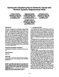
Figure 2. Strength changes against the number of features in the subspace on the 9 high dimensional datasets



Next we investigated the impact of the informative features on classification performance. The error bound indicator c/s2 and the accuracy on the test data is used to compare the three models for each dataset. A subspace size of  log 2 (M ) + 1 is used. Table 3 summarizes the results. “RF” stands for random forest with Breiman’s original method, and “New_RF” is random forest with our proposed method. We can see that our new random forest algorithm (irrespective of the choice of informativeness measure) always reduces the error bound and increases the classification accuracy on all datasets. The average increase in accuracy is 19% with a maximum increase of 56%, which is a remarkable improvement.

5.4. Performance Comparison on High Dimensional Data In this experiment we carried out a comprehensive analysis on the properties of the new random forest algorithm on the 9 real life high dimensional datasets and compared the results with those of Breiman’s random forest algorithm. We used different subspace sizes to build random forest models. For the new random forest algorithm, the two methods were used to compute the feature weights. In each subspace, we built 80 random forest models by each algorithm and calculated the average values of the four measures Strength, Correlation, c/s2, and Accuracy. We began with a subspace of 5 features. The performance of the three random forest algorithms on the four measures for each of the 9 datasets is shown in Figures 2, 3, 4, and 5. Figure 2 plots the strength for the three methods against different subspace sizes on each of the 9 datasets. The dark squares show the strength computed from Breiman’s algorithm. The dark triangles show the strengths by the new algorithm with IGR as the feature weights while the circles show the strengths with CS. In the same subspace, the higher the strength, the better the results. From the curves, we can see that the new algorithms consistently performed better than Breiman’s algo-

rithm. The advantages are more obvious in small subspaces. The new algorithms quickly achieved higher strength as the subspace size increased. Breiman’s algorithm requires larger subspaces to achieve a higher strength. These results indicate that the feature weighting method for subspace selection enables random forest models to achieve a higher strength for small subspace sizes compared to Breiman’s algorithm. Figure 3 plots the curves for the correlations for the three random forest methods on the 9 datasets. For small subspace sizes Breiman’s algorithm produces higher correlations between the trees on all datasets, except for Newsgroups. The correlation decreases as the subspace size increases. For the random forest models the lower the correlation between the trees then the better the final model. To achieve a low level of correlation for Breiman’s algorithm, a larger subspace size is generally required. With our new random forest algorithms a low correlation level is achieved with very small subspaces in all 9 datasets. We also note that as the subspace size increases the correlation level increases as well. This is understandable because as the subspace size increases, the same informative features are more likely to be selected repeatedly in the subspaces, increasing the similarity of the decision trees. Therefore, the feature weighting method for subspace selection works well for small subspaces, at least from the point of view of the correlation measure. Gisette and Newsgroups data sets are two special cases which require further investigation. Figure 4 shows the error bound indicator c/s2 for the three methods on the 9 datasets. From these figures we can observe that as the subspace size increases, c/s2 consistently reduces. The behaviour indicates that a subspace size larger than  log 2 (M ) + 1 benefits all three algorithms. However, the new algorithms achieve a lower level of c/s2 at subspace sizes of  log 2 (M ) + 1 than Breiman’s algorithm. To achieve the same level with Breiman’s algorithm we require the subspace size to be several times larger than  log 2 (M ) + 1 . This demonstrates



Figure 3. Correlation changes against the number of features in the subspace on the 9 high dimensional datasets



Figure 4. c/s2 changes against the number of features in the subspace on the 9 high dimensional datasets



Figure 5. Test Accuracy changes against the number of features in the subspace on the 9 high dimensional datasets



a clear advantage for the new algorithms in reducing computational costs. Finally Figure 5 plots the curves showing the accuracy of the three random forest models on the test datasets from the 9 datasets. Similar to c/s2, the accuracy of models produced using Breiman’s algorithm is low for small subspaces. In the subspace of  log 2 (M ) + 1 features the new algorithms achieve higher accuracy. To achieve the same level of accuracy Breiman’s algorithm requires a much larger subspace. These results illustrate that the subspace formula  log 2 (M ) + 1 in very high dimensional data remains valid for the new algorithms. However, it is no longer valid for Breiman’s algorithm. A much larger subspace is required, and the actual subspace size for accurate models is different for the different datasets. In practice, it is difficult to determine a subspace size for high dimensional data when using Breiman’s algorithm. Instead, with our new algorithms, we can retain the use of  log 2 (M ) + 1 as the subspace size, even for high dimensional data. This is a major result from our research.

6. CONCLUSION AND FURTHER WORK In this paper we have presented a feature weighting method for subspace selection for building random forest models using high dimensional data. We have presented a new random forest algorithm that incorporates the new subspace selection method. The algorithm can be used to classify multi-class data and can retain a small subspace size to create accurate random forest models-we retain Breiman’s formula  log 2 (M ) + 1 for determining the subspace size. For high dimensional data this formula is no longer valid for Breiman’s algorithm because the subspace size is shown empirically to be too small and produces less optional models. Building random forest models from large high dimensional data presents computational challenges. Our new algorithms address this to some extent, by limiting the subspace size

without compromising (and in fact improving) model performance. Our future work is exploring distributed solutions to make use of cloud computing to implement the new random forest algorithm to tackle very large data problems.

ACKNOWLEDGMENT This research is supported in part by NSFC under Grant NO.61073195, and Shenzhen New Industry Development Fund under Grant NO.CXB201005250021A. The source codes, executable programs, datasets, and other instructions about our experimentations can be downloaded from the IJDWM source codes official website at: http://users.monash. edu/~dtaniar/IJDWM/

REFERENCES Amaratunga, D., Cabrera, J., & Lee, Y. S. (2008). Enriched random forests. Bioinformatics (Oxford, England), 24(18), 2010–2014. doi:10.1093/bioinformatics/btn356 Asuncion, A., & Newman, D. J. (2010). UCI machine learning repository. Retrieved June 1, 2010, from http://www.ics.uci.edu/~mlearn/MLRepository.html Banfield, R. E., Hall, L. O., Bowyer, K. W., & Kegelmeyer, W. P. (2007). A comparison of decision tree ensemble creation techniques. IEEE Transactions on Pattern Analysis and Machine Intelligence, 29(1), 173–180. doi:10.1109/TPAMI.2007.250609 Bosch, A., Zisserman, A., & Muoz, X. (2007). Image classification using random forests and ferns. In Proceedings of the IEEE International Conference on Computer Vision (pp. 1-8). Breiman, L. (2001). Random forests. Machine Learning, 45(1), 5–32. doi:10.1023/A:1010933404324 Bureau, A., Dupuis, J., Falls, K., Lunetta, K. L., Hayward, B., Keith, T. P., & Eerdewegh, P. V. (2005). Identifying SNPs predictive of phenotype using random forests. Genetic Epidemiology, 28(2), 171–182. doi:10.1002/gepi.20041 Chen, X. W., & Liu, M. (2005). Prediction of protein-protein interactions using random decision forest framework. Bioinformatics (Oxford, England), 21(24), 4394. doi:10.1093/bioinformatics/bti721



Diaz-Uriarte, R., & De Andres, S. A. (2006). Gene selection and classification of microarray data using random forest. BMC Bioinformatics, 7(1), 3. doi:10.1186/1471-2105-7-3 Dietterich, T. G. (2000). An experimental comparison of three methods for constructing ensembles of decision trees: Bagging, boosting, and randomization. Machine Learning, 40(2), 139–157. doi:10.1023/A:1007607513941 Engle, K. M., & Gangopadhyay, A. (2010). An efficient method for discretizing continuous attributes. International Journal of Data Warehousing and Mining, 6(2), 1–21. doi:10.4018/jdwm.2010040101 Freund, Y., & Schapire, R. E. (1996). Experiments with a new boosting algorithm. In Proceedings of the Thirteenth International Conference on Machine Learning (pp. 148-156). Han, E. H., Boley, D., Gini, M., Gross, R., Hastings, K., Karypis, G., et al. (1998). WebACE: A web agent for document categorization and exploration. In Proceedings of the 2nd International Conference on Autonomous Agents (pp. 408-415). Han, E. H., & Karypis, G. (2000). Centroid-based document classification: Analysis & experimental results. In Proceedings of the Fourth European Conference on Principles Data Mining and Knowledge (pp. 424-431). Ho, T. K. (1995). Random decision forest. In Proceedings of the Third International Conference on Document Analysis and Recognition (pp. 278-282). Ho, T. K. (1998). The random subspace method for constructing decision forests. IEEE Transactions on Pattern Analysis and Machine Intelligence, 20(8), 832–844. doi:10.1109/34.709601 LeCun, Y., & Cortes, C. (2010). The MNST database. Retrieved October 13, 2010, from http://yann.lecun. com/exdb/mnist/index.html Lewis, D. D. (1999). Reuters-21578 text categorization test collection distribution 1.0. Retrieved June 1, 2010, from http://www.research.att.com/~lewis

Li, J. (2010). Kent Ridge bio-medical data set repository. Retrieved June 1, 2010, from http://levis.tongji. edu.cn/gzli/data/mirror-kentridge.html Liu, H., & Wong, L. (2003). Data mining tools for biological sequences. Journal of Bioinformatics and Computational Biology, 1(1), 139–167. doi:10.1142/ S0219720003000216 Pang, H., Lin, A., Holford, M., Enerson, B. E., Lu, B., & Lawton, M. P. (2006). Pathway analysis using random forests classification and regression. Bioinformatics (Oxford, England), 22(16), 2028–2036. doi:10.1093/bioinformatics/btl344 Pearson, K. (1904). On the theory of contingency and its relation to association and normal correlation. Cambridge, UK: Cambridge University Press. Qiu, D., Wang, Y., & Bi, B. (2008). Identify crossselling opportunities via hybrid classifier. International Journal of Data Warehousing and Mining, 4(2), 55–62. doi:10.4018/jdwm.2008040107 Quinlan, J. R. (1993). C4.5: Programs for machine learning. San Francisco, CA: Morgan Kaufmann. Quinlan, J. R. (1996). Improved use of continuous attributes in C4.5. Journal of Artificial Intelligence Research, 4, 77–90. Rennie, J. (2008). Tom Mitchell. Retrieved June 1, 2010, from http://people.csail.mit.edu/ jrennie/20Newsgroups/20news-bydate-matlab.tgz Saxena, A., & Wang, J. (2010). Dimensionality reduction with unsupervised feature selection and applying non-Euclidean norms for classification accuracy. International Journal of Data Warehousing and Mining, 6(2), 22–40. doi:10.4018/jdwm.2010040102 Ward, M. M., Pajevic, S., Dreyfuss, J., & Malley, J. D. (2006). Short-term prediction of mortality in patients with systemic lupus erythematosus: classification of outcomes using random forests. Arthritis and Rheumatism, 55(1), 74–80. doi:10.1002/art.21695 Ye, Y., Li, H., Deng, X., & Huang, J. Z. (2008). Feature weighting random forest for detection of hidden web search interfaces. Computational Linguistics and Chinese Language Processing, 13(4), 387–404.



Baoxun Xu is a PhD student in the Department of Computer Science, Harbin Institute of Technology Shenzhen Graduate School, He received the BS degree in information management and information system from Harbin University of Science & Technology, China in 2004 and MS in software engineering from Harbin Institute of Technology, China in 2007. His current research interests include classification algorithm, text categorization, and parallel algorithm. Joshua Zhexue Huang received his PhD Degree in Spatial Databases from the Royal Institute of Technology, Stockholm, Sweden, 1993. He is presently a Professor in Shenzhen Institutes of Advanced Technology, Chinese Academy of Sciences. His research interests are in database, data mining, pattern recognition, machine learning, and grid computing. He has published over 100 papers in international journals and conference proceedings in these areas. He served in various technical program committees of international conferences in related areas. Graham Williams received his PhD Degree in Computer Science from Australian National University. Canberra, Australia, 1991. He is presently a Visiting Professor in Shenzhen Institutes of Advanced Technology, Chinese Academy of Sciences. His research interests are in ensemble models, social network analysis, high performance computing and open source software and freedom in computing. He has published more than 100 peer reviewed research papers in various journals, conferences, and books. Qiang Wang is a PhD student in the Department of Computer Science, Harbin Institute of Technology Shenzhen Graduate School, He received his B.S degree and MS degree in computer science from YanShan University, in 2000 and 2003, respectively. His current research interests are in the areas of data mining, clustering algorithm with application, bioinformatics. Yunming Ye received the PhD degree in computer science from Shanghai Jiao Tong University, China, in 2004. He received the MS degree in computer science from Fuzhou University, China in 2001. He is currently a professor of the Department of Computer Science at Harbin Institute of Technology Shenzhen Graduate School. His major research fields are data mining and web search technology.


Classifying Very High-Dimensional Data with Random Forests Built ...

Classifying Very High-Dimensional Data with Random Forests Built ...

Suggest Documents

Classifying Very High-Dimensional Data with Random ... - Togaware

Classifying very-high-dimensional data with ... - Semantic Scholar

Earthquake Classifying Neural Networks Trained with Random

Improving Credit Scoring with Random Forests

Dynamic Integration with Random Forests - CiteSeerX

Towards Image Colorization with Random Forests - SciTePress

Random survival forests - arXiv

Banzhaf Random Forests

RANDOM FORESTS FOR BEGINNERS

Random Forests is

Calibrating Random Forests

Classifying the Built-Up Structure of Urban Blocks with ... - MDPI

Classifying Complex Mountainous Forests with L ... - Semantic Scholar

Diversified Random Forests Using Random Subspaces

Random Multiclass Classification: Generalizing Random Forests to

Classifying Complex Mountainous Forests with L-Band SAR ... - MDPI

Classifying Northern Forests Using Thematic Mapper ...

Random Forests for Laughter Detection

Random Forests - Temple University [PDF]

Distributed Stochastic Aware Random Forests-Efficient Data Mining for ...

Graph Propositionalization for Random Forests

Spatiotemporal Relational Random Forests - CiteSeerX

On-line Random Forests - CiteSeerX

'Random Forests' Classifier - Semantic Scholar